
Evaluation of Rainfall Erosivity in the Western Balkans by Mapping and Clustering ERA5 Reanalysis Data

 ,
,  ,
,  ,
, 
 ,
,  ,
,  , , and
Abstract
1. Introduction
2. Materials and Methods
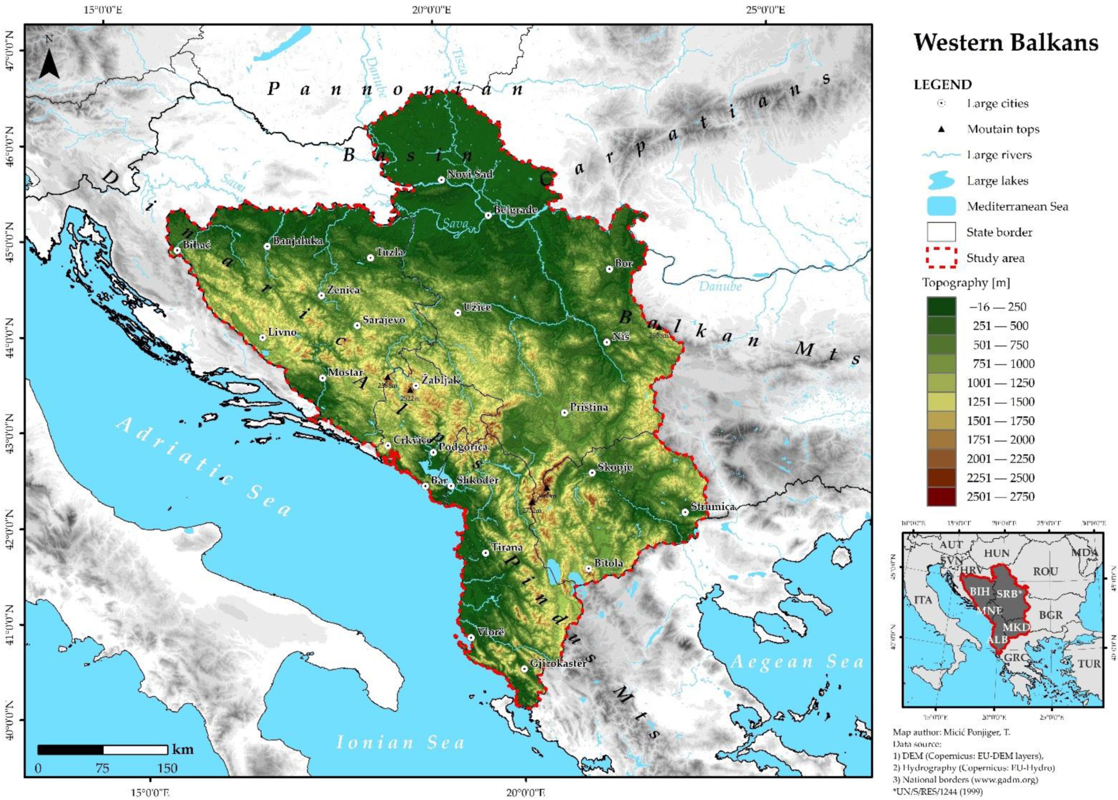
2.1. Study Area
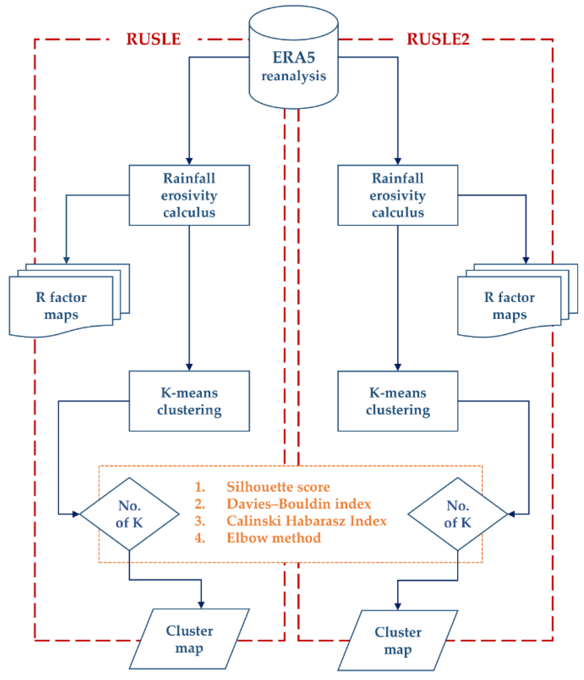
2.2. Methodology
2.2.1. Database
2.2.2. Rainfall Erosivity: R-Factor Calculation
2.2.3. k-Means Clustering
3. Results and Discussion
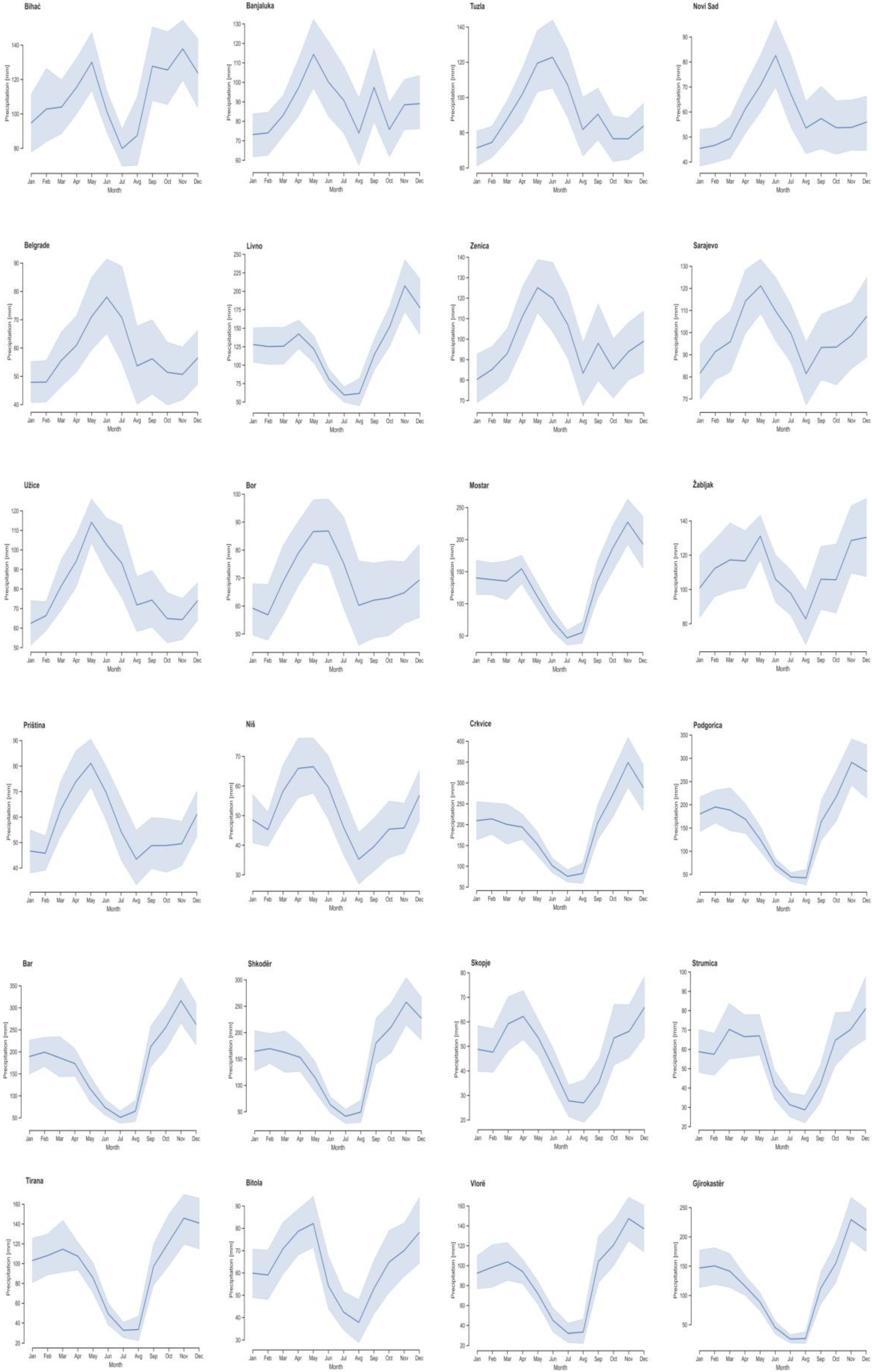
3.1. Precipitation Variation
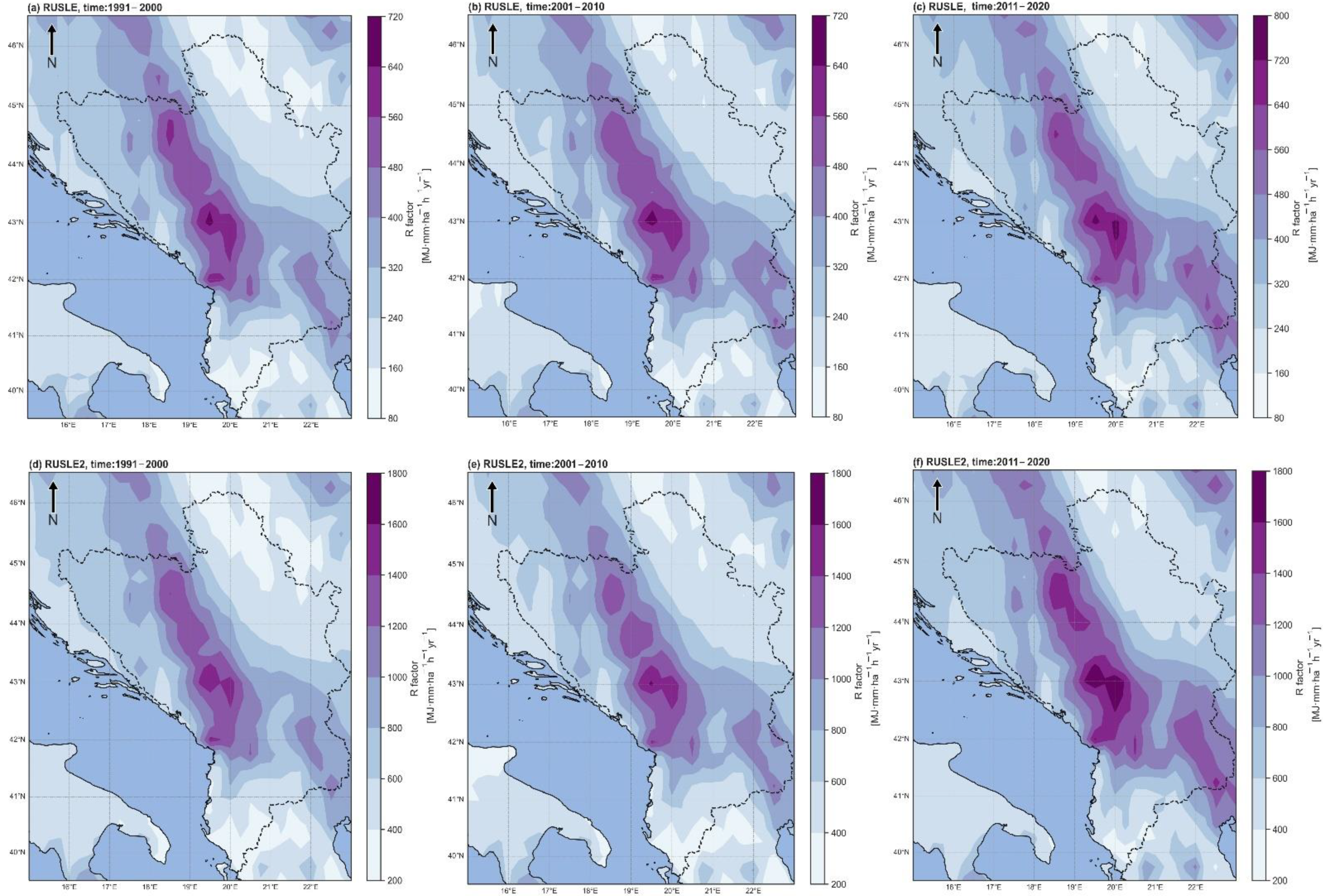
3.2. R-Factor Variability
3.3. Clustering
3.4. Policy, Practical Implications and Study Limitations
4. Conclusions
Author Contributions
Funding
Institutional Review Board Statement
Informed Consent Statement
Data Availability Statement
Acknowledgments
Conflicts of Interest
Appendix A

Appendix B


References
- Daskalov, R.D.; Mishkova, D.; Marinov, T.; Vezenkov, A. Entangled Histories of the Balkans—Volume Four; BRILL: Leiden, The Netherlands, 2017; ISBN 9789004337824. [Google Scholar]
- Vuković, A.; Mandić, M.V. Study on Climate Change in the Western Balkans Region; Regional Cooperation Council Secretariat: Sarajevo, Bosnia and Herzegovina, 2018. [Google Scholar]
- Füssel, H.-M.; Jol, A.; Marx, A.; Hildén, M. (Eds.) Climate Change, Impacts and Vulnerability in Europe 2016: An Indicator-Based Report; European Environment Agency: Copenhagen, Denmark, 2017; ISBN 1977-8449. [Google Scholar]
- Blinkov, I. Review and Comparison of Water Erosion Intensity in the Western Balkan and Eu Countries. Contrib. Sect. Nat. Math. Biotech. Sci. 2017, 36, 27–42. [Google Scholar] [CrossRef][Green Version]
- Verheijen, F.G.A.; Jones, R.J.A.; Rickson, R.J.; Smith, C.J. Tolerable versus actual soil erosion rates in Europe. Earth-Sci. Rev. 2009, 94, 23–38. [Google Scholar] [CrossRef]
- Gavrilović, S. Inženjering o Bujičnim Tokovima i Erozij (on Serbian); Izgradnja: Beograd, Serbian, 1972; pp. 1–292. [Google Scholar]
- Milanesi, L.; Pilotti, M.; Clerici, A.; Gavrilovic, Z. Application of an improved version of the erosion potential method in alpine areas. Ital. J. Eng. Geol. Environ. 2015, 1, 17–30. [Google Scholar]
- Kostadinov, S.; Zlatic, M.; Nada, D.; Gavrilovic, Z. Serbia and Montenegro. In Soil Erosion in Europe; Boardman, J., Poesen, J., Eds.; Wiley: Chichester, UK, 2006; pp. 271–277. [Google Scholar]
- Efthimiou, N.; Lykoudi, E.; Panagoulia, D.; Karavitis, C. Assessment of soil susceptibility to erosion using the EPM and RUSLE Models: The case of Venetikos River Catchment. Glob. NEST J. 2016, 18, 164–179. [Google Scholar]
- Globevnik, L.; Holjevic, D.; Petkovsek, G.; Rubinic, J. Applicability of the Gavrilovic method in erosion calculation using spatial data manipulation techniques. Int. Assoc. Hydrol. Sci. 2003, 297, 224–233. [Google Scholar]
- Dragičević, N.; Karleuša, B.; Ožanić, N. Erosion Potential Method (Gavrilović method) sensitivity analysis. Soil Water Res. 2017, 12, 51–59. [Google Scholar] [CrossRef]
- Boardman, J.; Poesen, J. Grazhdani Albania. In Soil Erosion in Europe; Boardman, J., Poesen, J., Eds.; Wiley & Sons: New York, NY, USA, 2006. [Google Scholar]
- Tošić, R.; Dragićevic, S.; Kostadinov, S.; Dragović, N. Assessment of soil erosion potential by the USLE method: Case study, Republic of Srpska—BiH. Fresenius Environ. Bull. 2011, 20, 1910–1917. [Google Scholar]
- Tošić, R.; Dragićević, S.; Lovrić, N. Assessment of soil erosion and sediment yield changes using erosion potential model—Case study: Republic of Srpska (BiH). Carpathian J. Earth Environ. Sci. 2012, 7, 147–154. [Google Scholar]
- Panagos, P.; Ballabio, C.; Borrelli, P.; Meusburger, K.; Klik, A.; Rousseva, S.; Tadić, M.P.; Michaelides, S.; Hrabalíková, M.; Olsen, P.; et al. Rainfall erosivity in Europe. Sci. Total Environ. 2015, 511, 801–814. [Google Scholar] [CrossRef]
- Panagos, P.; Meusburger, K.; Ballabio, C.; Borrelli, P.; Beguería, S.; Klik, A.; Rymszewicz, A.; Michaelides, S.; Olsen, P.; Tadić, M.P.; et al. Reply to the comment on “Rainfall erosivity in Europe” by Auerswald et al. Sci. Total Environ. 2015, 532, 853–857. [Google Scholar] [CrossRef] [PubMed]
- Panagos, P.; Borrelli, P.; Spinoni, J.; Ballabio, C.; Meusburger, K.; Beguería, S.; Klik, A.; Michaelides, S.; Petan, S.; Hrabalíková, M.; et al. Monthly Rainfall Erosivity: Conversion Factors for Different Time Resolutions and Regional Assessments. Water 2016, 8, 119. [Google Scholar] [CrossRef]
- Ballabio, C.; Borrelli, P.; Spinoni, J.; Meusburger, K.; Michaelides, S.; Beguería, S.; Klik, A.; Petan, S.; Janeček, M.; Olsen, P.; et al. Mapping monthly rainfall erosivity in Europe. Sci. Total Environ. 2017, 579, 1298–1315. [Google Scholar] [CrossRef] [PubMed]
- Bezak, N.; Ballabio, C.; Mikoš, M.; Petan, S.; Borrelli, P.; Panagos, P. Reconstruction of past rainfall erosivity and trend detection based on the REDES database and reanalysis rainfall. J. Hydrol. 2020, 590, 125372. [Google Scholar] [CrossRef]
- Bezak, N.; Borrelli, P.; Panagos, P. A first assessment of rainfall erosivity synchrony scale at pan-European scale. Catena 2021, 198, 105060. [Google Scholar] [CrossRef]
- Diodato, N.; Borrelli, P.; Panagos, P.; Bellocchi, G. Global assessment of storm disaster-prone areas. PLoS ONE 2022, 17, e0272161. [Google Scholar] [CrossRef]
- Borrelli, P.; Alewell, C.; Alvarez, P.; Anache, J.A.A.; Baartman, J.; Ballabio, C.; Bezak, N.; Biddoccu, M.; Cerdà, A.; Chalise, D.; et al. Soil erosion modelling: A global review and statistical analysis. Sci. Total Environ. 2021, 780, 146494. [Google Scholar] [CrossRef]
- Padulano, R.; Rianna, G.; Santini, M. Datasets and approaches for the estimation of rainfall erosivity over Italy: A comprehensive comparison study and a new method. J. Hydrol. Reg. Stud. 2021, 34, 100788. [Google Scholar] [CrossRef]
- Tošić, R.; Kapović Solomun, M.; Lovrić, N.; Dragicević, S. Assessment of soil erosion potential using RUSLE and GIS: A case study of Bosnia and Herzegovina. Fresenius Environ. Bull. 2013, 22, 3415–3423. [Google Scholar]
- Milanović, M.M.; Perović, V.S.; Tomić, M.D.; Lukić, T.; Nenadović, S.S.; Radovanović, M.M.; Ninković, M.M.; Samardžić, I.; Miljković, Đ. Analysis of the state of vegetation in the municipality of Jagodina (Serbia) through remote sensing and suggestions for protection. Geogr. Pannonica 2016, 20, 70–78. [Google Scholar] [CrossRef]
- Perović, V.; Životić, L.; Kadović, R.; Đorđević, A.; Jaramaz, D.; Mrvic, V.; Todorović, M. Spatial modelling of soil erosion potential in a mountainous watershed of South-eastern Serbia. Environ. Earth Sci. 2013, 68, 115–128. [Google Scholar] [CrossRef]
- Perović, V.; Jakšić, D.; Jaramaz, D.; Koković, N.; Čakmak, D.; Mitrović, M.; Pavlović, P. Spatio-temporal analysis of land use/land cover change and its effects on soil erosion (Case study in the Oplenac wine-producing area, Serbia). Environ. Monit. Assess. 2018, 190, 675. [Google Scholar] [CrossRef] [PubMed]
- Perović, V.; Čakmak, D.; Mitrović, M.; Pavlović, P. The Potential Impact of Climate Change and Land Use on Future Soil Erosion, Based on the Example of Southeast Serbia. In Advances in Understanding Soil Degradation; Springer: Cham, Switzerland, 2022; pp. 207–228. [Google Scholar]
- Agaj, T.; Bytyqi, V. Analysis of Soil Erosion Risk in a River Basin—A Case Study from Hogoshti River Basin (Kosovo). Ecol. Eng. Environ. Technol. 2022, 23, 162–171. [Google Scholar] [CrossRef]
- Miftari, L.; Gjoka, F.; Toromani, E. Assessment of soil loss in watershed of location in Ulza Basin, Albania. J. Balk. Ecol. 2018, 21, 400–413. [Google Scholar]
- Zdruli, P.; Karydas, C.G.; Dedaj, K.; Salillari, I.; Cela, F.; Lushaj, S.; Panagos, P. High resolution spatiotemporal analysis of erosion risk per land cover category in Korçe region, Albania. Earth Sci. Inform. 2016, 9, 481–495. [Google Scholar] [CrossRef]
- Nikolova, E. Soil Erosion Modeling Using RUSLE and GIS in the Republic of Macedonia; Polytechnic University of Milan: Milan, Italy, 2016. [Google Scholar]
- Blinkov, I.; Kostadinov, S.; Marinov, I.T. Comparison of erosion and erosion control works in Macedonia, Serbia and Bulgaria. Int. Soil Water Conserv. Res. 2013, 1, 15–28. [Google Scholar] [CrossRef]
- Golijanin, J.; Nikolić, G.; Valjarević, A.; Ivanović, R.; Tunguz, V.; Bojić, S.; Grmuša, M.; Lukić Tanović, M.; Perić, M.; Hrelja, E.; et al. Estimation of potential soil erosion reduction using GIS-based RUSLE under different land cover management models: A case study of Pale Municipality, B&H. Front. Environ. Sci. 2022, 10, 1257. [Google Scholar] [CrossRef]
- Milentijević, N.; Ostojić, M.; Fekete, R.; Kalkan, K.; Ristić, D.; Bačević, N.; Stevanović, V.; Pantelić, M. Assessment of Soil Erosion Rates Using Revised Universal Soil Loss Equation (RUSLE) and GIS in Bačka (Serbia). Pol. J. Environ. Stud. 2021, 30, 5175–5184. [Google Scholar] [CrossRef]
- Lukić, T.; Lukić, A.; Basarin, B.; Ponjiger, T.M.; Blagojević, D.; Mesaroš, M.; Milanović, M.; Gavrilov, M.; Pavić, D.; Zorn, M.; et al. Rainfall erosivity and extreme precipitation in the Pannonian basin. Open Geosci. 2019, 11, 664–681. [Google Scholar] [CrossRef]
- Lukić, T.; Micić Ponjiger, T.; Basarin, B.; Sakulski, D.; Gavrilov, M.; Marković, S.; Zorn, M.; Komac, B.; Milanović, M.; Pavić, D.; et al. Application of Angot precipitation index in the assessment of rainfall erosivity: Vojvodina Region case study (North Serbia). Acta Geogr. Slov. 2021, 61, 123–153. [Google Scholar] [CrossRef]
- Perović, V.; Đorđević, A.; Životić, L.; Nikolić, N.; Kadović, R.; Belanović, S. Soil Erosion Modelling in the Complex Terrain of Pirot Municipality. Carpathian J. Earth Environ. Sci. 2012, 7, 93–100. [Google Scholar]
- Belanović, S.; Perović, V.; Vidojević, D.; Kostadinov, S.; Knežević, M.; Kadović, R.; Košanin, O. Assessment of soil erosion intensity in Kolubara District, Serbia. Fresenius Environ. Bull. 2013, 22, 1556–1563. [Google Scholar]
- Životić, L.; Perović, V.; Jaramaz, D.; Đorđević, A.; Petrović, R.; Todorović, M. Application of USLE, GIS, and Remote Sensing in the Assessment of Soil Erosion Rates in Southeastern Serbia. Pol. J. Environ. Stud. 2012, 21, 1929–1935. [Google Scholar]
- Perović, V.; Kostadinov, S.; Jaramaz, D.; Kadović, R. Overview of the most important models for the soil loss assessment due to water erosion. Geonauka 2013, 1, 6–11. [Google Scholar] [CrossRef][Green Version]
- Micić Ponjiger, T.; Lukić, T.; Basarin, B.; Jokić, M.; Wilby, R.L.; Pavić, D.; Mesaroš, M.; Valjarević, A.; Milanović, M.M.; Morar, C. Detailed Analysis of Spatial–Temporal Variability of Rainfall Erosivity and Erosivity Density in the Central and Southern Pannonian Basin. Sustainability 2021, 13, 13355. [Google Scholar] [CrossRef]
- Wilby, R.L.; Yu, D. Rainfall and temperature estimation for a data sparse region. Hydrol. Earth Syst. Sci. 2013, 17, 3937–3955. [Google Scholar] [CrossRef]
- Jiao, D.; Xu, N.; Yang, F.; Xu, K. Evaluation of spatial-temporal variation performance of ERA5 precipitation data in China. Sci. Rep. 2021, 11, 17956. [Google Scholar] [CrossRef] [PubMed]
- Nogueira, M. Inter-comparison of ERA-5, ERA-interim and GPCP rainfall over the last 40 years: Process-based analysis of systematic and random differences. J. Hydrol. 2020, 583, 124632. [Google Scholar] [CrossRef]
- Matkovski, B.; Zekić, S.; Đokić, D.; Jurjević, Ž.; Đurić, I. Export Competitiveness of Agri-Food Sector during the EU Integration Process: Evidence from the Western Balkans. Foods 2021, 11, 10. [Google Scholar] [CrossRef]
- Panagos, P.; Montanarella, L.; Barbero, M.; Schneegans, A.; Aguglia, L.; Jones, A. Soil priorities in the European Union. Geoderma Reg. 2022, 29, e00510. [Google Scholar] [CrossRef]
- IPCC. Climate Change 2022: Impacts, Adaptation and Vulnerability. Contribution of Working Group II to the Sixth Assessment Report of the Intergovernmental Panel on Climate Change; Pörtner, H.O., Roberts, D.C., Tignor, M., Poloczanska, E.S., Mintenbeck, K., Alegría, A., Craig, M., Langsdorf, S., Löschke, S., Möller, V., et al., Eds.; Cambridge University Press: Cambridge, UK; New York, NY, USA, 2022. [Google Scholar]
- Knez, S.; Štrbac, S.; Podbregar, I. Climate change in the Western Balkans and EU Green Deal: Status, mitigation and challenges. Energy Sustain. Soc. 2022, 12, 1. [Google Scholar] [CrossRef]
- Orgiazzi, A.; Panagos, P.; Fernández-Ugalde, O.; Wojda, P.; Labouyrie, M.; Ballabio, C.; Franco, A.; Pistocchi, A.; Montanarella, L.; Jones, A. LUCAS Soil Biodiversity and LUCAS Soil Pesticides, new tools for research and policy development. Eur. J. Soil Sci. 2022, 73, e13299. [Google Scholar] [CrossRef]
- Panagos, P.; Borrelli, P.; Matthews, F.; Liakos, L.; Bezak, N.; Diodato, N.; Ballabio, C. Global rainfall erosivity projections for 2050 and 2070. J. Hydrol. 2022, 610, 127865. [Google Scholar] [CrossRef]
- Reed, J.M.; Kryštufek, B.; Eastwood, W.J. The Physical Geography of The Balkans and Nomenclature of Place Names. In Balkan Biodiversity; Springer Netherlands: Dordrecht, The Netherlands, 2004; pp. 9–22. [Google Scholar]
- Tošić, I. Spatial and temporal variability of winter and summer precipitation over Serbia and Montenegro. Theor. Appl. Climatol. 2004, 77, 47–56. [Google Scholar] [CrossRef]
- Papić, D.; Bačević, N.R.; Valjarević, A.; Milentijević, N.; Gavrilov, M.B.; Živković, M.; Marković, S.B. Assessment of air temperature trend in South and Southeast Bosnia and Herzegovina from 1961 to 2017. Időjárás 2020, 124, 381–399. [Google Scholar] [CrossRef]
- Porja, T. Heat Waves Affecting Weather and Climate over Albania. J. Earth Sci. Clim. Chang. 2013, 4, 4. [Google Scholar] [CrossRef]
- Monevska, S.A. Climate Changes in Republic of Macedonia. In Climate Change and Its Effects on Water Resources; Baba, A., Tayfur, G., Gündüz, O., Howard, K., Friedel, M., Chambel, A., Eds.; Springer: Dordrecht, The Netherlands, 2011; pp. 203–213. [Google Scholar]
- Tošić, I.; Hrnjak, I.; Gavrilov, M.B.; Unkašević, M.; Marković, S.B.; Lukić, T. Annual and seasonal variability of precipitation in Vojvodina, Serbia. Theor. Appl. Climatol. 2014, 117, 331–341. [Google Scholar] [CrossRef]
- Hrnjak, I.; Lukić, T.; Gavrilov, M.B.; Marković, S.B.; Unkašević, M.; Tošić, I. Aridity in Vojvodina, Serbia. Theor. Appl. Climatol. 2014, 115, 323–332. [Google Scholar] [CrossRef]
- Gavrilov, M.; Markovic, S.; Jarad, A.; Korac, V. The analysis of temperature trends in Vojvodina (Serbia) from 1949 to 2006. Therm. Sci. 2015, 19, 339–350. [Google Scholar] [CrossRef]
- Gavrilov, M.B.M.B.; Radaković, M.G.M.G.; Sipos, G.; Mezősi, G.; Gavrilov, G.; Lukić, T.; Basarin, B.; Benyhe, B.; Fiala, K.; Kozák, P.; et al. Aridity in the Central and Southern Pannonian Basin. Atmosphere 2020, 11, 1269. [Google Scholar] [CrossRef]
- Radaković, M.G.; Tošić, I.; Bačević, N.; Mladjan, D.; Gavrilov, M.B.; Marković, S.B. The analysis of aridity in Central Serbia from 1949 to 2015. Theor. Appl. Climatol. 2018, 133, 887–898. [Google Scholar] [CrossRef]
- Gavrilov, M.B.; Marković, S.B.; Janc, N.; Nikolić, M.; Valjarević, A.; Komac, B.; Zorn, M.; Punišić, M.; Bačević, N. Assessing average annual air temperature trends using the Mann–Kendall test in Kosovo. Acta Geogr. Slov. 2018, 58, 7–25. [Google Scholar] [CrossRef]
- Barry, R.G.; Chorley, R.J. Atmosphere, Weather and Climate, 7’11 ed.; Routledge: London, UK, 1998. [Google Scholar]
- Varlas, G.; Stefanidis, K.; Papaioannou, G.; Panagopoulos, Y.; Pytharoulis, I.; Katsafados, P.; Papadopoulos, A.; Dimitriou, E. Unravelling Precipitation Trends in Greece since 1950s Using ERA5 Climate Reanalysis Data. Climate 2022, 10, 12. [Google Scholar] [CrossRef]
- Bandhauer, M.; Isotta, F.; Lakatos, M.; Lussana, C.; Båserud, L.; Izsák, B.; Szentes, O.; Tveito, O.E.; Frei, C. Evaluation of daily precipitation analyses in E-OBS (v19.0e) and ERA5 by comparison to regional high-resolution datasets in European regions. Int. J. Climatol. 2022, 42, 727–747. [Google Scholar] [CrossRef]
- Bezak, N.; Borrelli, P.; Panagos, P. Exploring the possible role of satellite-based rainfall data in estimating inter- and intra-annual global rainfall erosivity. Hydrol. Earth Syst. Sci. 2022, 26, 1907–1924. [Google Scholar] [CrossRef]
- Hersbach, H.; Bell, B.; Berrisford, P.; Hirahara, S.; Horányi, A.; Muñoz-Sabater, J.; Nicolas, J.; Peubey, C.; Radu, R.; Schepers, D.; et al. The ERA5 global reanalysis. Q. J. R. Meteorol. Soc. 2020, 146, 1999–2049. [Google Scholar] [CrossRef]
- Petan, S.; Rusjan, S.; Vidmar, A.; Mikoš, M. The rainfall kinetic energy–intensity relationship for rainfall erosivity estimation in the mediterranean part of Slovenia. J. Hydrol. 2010, 391, 314–321. [Google Scholar] [CrossRef]
- Renard, K.G.K.; Foster, G.R.G.; Weesies, G.A.G.; McCool, D.K.; Yoder, D.C.D. Predicting soil erosion by water: A guide to conservation planning with the revised universal soil loss equation (RUSLE). In U.S. Department of Agriculture, Agriculture Handbook; ARS: Washington, DC, USA, 1997; Volume 703, p. 404. ISBN 0160489385. [Google Scholar]
- USDA. Draft Science Documentation: Revised Universal Soil Loss Equation Version 2 (RUSLE2); USDA-Agricultural Research Service: Washington, DC, USA, 2008.
- Wischmeier, W.H. A rainfall erosion index for a universal soil-loss equation. Soil Sci. Soc. Am. J. 1959, 23, 246–249. [Google Scholar] [CrossRef]
- Brown, L.C.; Foster, G.R. Storm erosivity using idealized intensity distributions. Am. Soc. Agric. Biol. Eng. 1987, 30, 379–386. [Google Scholar] [CrossRef]
- Vantas, K.; Sidiropoulos, E.; Evangelides, C. Rainfall Erosivity and Its Estimation: Conventional and Machine Learning Methods. In Soil Erosion—Rainfall Erosivity and Risk Assessment; IntechOpen: London, UK, 2019. [Google Scholar]
- Raj, R.; Saharia, M.; Chakma, S.; Rafieinasab, A. Mapping rainfall erosivity over India using multiple precipitation datasets. Catena 2022, 214, 106256. [Google Scholar] [CrossRef]
- Kinnell, P.I.A. Rainfall Intensity-Kinetic Energy Relationships for Soil Loss Prediction1. Soil Sci. Soc. Am. J. 1981, 45, 153–155. [Google Scholar] [CrossRef]
- Rosewell, C.J. Rainfall kinetic energy in eastern Australia. J. Clim. Appl. Meteorol. 1986, 25, 1695–1701. [Google Scholar] [CrossRef]
- McGregor, K.C.; Mutchler, C.K. Status of the R factor in northern Mississippi. In Soil Erosion: Prediction and Control; Soil and Water Conservation Society: Ankeny, IA, USA, 1976; pp. 135–142. [Google Scholar]
- McGregor, K.C.; Bingner, R.L.; Bowie, A.J.; Foster, G.R. Erosivity index values for northern Mississippi. Trans. ASAE 1995, 38, 1039–1047. [Google Scholar] [CrossRef]
- Nearing, M.A.; Yin, S.; Borrelli, P.; Polyakov, V.O. Rainfall erosivity: An historical review. Catena 2017, 157, 357–362. [Google Scholar] [CrossRef]
- Panagos, P.; Borrelli, P.; Poesen, J.; Ballabio, C.; Lugato, E.; Meusburger, K.; Montanarella, L.; Alewell, C. The new assessment of soil loss by water erosion in Europe. Environ. Sci. Policy 2015, 54, 438–447. [Google Scholar] [CrossRef]
- Borrelli, P.; Diodato, N.; Panagos, P. Rainfall erosivity in Italy: A national scale spatio-temporal assessment. Int. J. Digit. Earth 2016, 9, 835–850. [Google Scholar] [CrossRef]
- Dash, C.J.; Das, N.K.; Adhikary, P.P. Rainfall erosivity and erosivity density in Eastern Ghats Highland of east India. Nat. Hazards 2019, 97, 727–746. [Google Scholar] [CrossRef]
- Bock, H.-H. Clustering Methods: A History of k-Means Algorithms. In Selected Contributions in Data Analysis and Classification; Springer: New York, NY, USA, 2007; pp. 161–172. [Google Scholar] [CrossRef]
- Lloyd, S.P. Least Squares Quantization in PCM. IEEE Trans. Inf. Theory 1982, 28, 129–137. [Google Scholar] [CrossRef]
- Arthur, D.; Vassilvitskii, S. K-Means++: The Advantages of Careful Seeding. In Proceedings of the Eighteenth Annual ACM-SIAM Symposium on Discrete Algorithms; Society for Industrial and Applied Mathematics: Philadelphia, PA, USA, 2007; pp. 1027–1035. [Google Scholar]
- Calinski, T.; Harabasz, J. Communications in Statistics A dendrite method for cluster analysis. Commun. Stat. 1974, 3, 1–27. [Google Scholar]
- Davies, D.L.; Bouldin, D.W. A Cluster Separation Measure. IEEE Trans. Pattern Anal. Mach. Intell. 1979, PAMI-1, 224–227. [Google Scholar] [CrossRef]
- Rousseeuw, P.J. Silhouettes: A graphical aid to the interpretation and validation of cluster analysis. J. Comput. Appl. Math. 1987, 20, 53–65. [Google Scholar] [CrossRef]
- Thorndike, R.L. Who belongs in the family? Psychometrika 1953, 18, 267–276. [Google Scholar] [CrossRef]
- Pedregosa, F.; Varoquaux, G.; Gramfort, A.; Michel, V.; Thirion, B.; Grisel, O.; Blondel, M.; Prettenhofer, P.; Weiss, R.; Dubourg, V.; et al. Scikit-learn: Machine Learning in Python. J. Mach. Learn. Res. 2011, 12, 2825–2830. [Google Scholar]
- Hunter, J.D. Matplotlib: A 2D Graphics Environment. Comput. Sci. Eng. 2007, 9, 90–95. [Google Scholar] [CrossRef]
- Waskom, M.; Botvinnik, O.; O’Kane, D.; Hobson, P.; Lukauskas, S.; Gemperline, D.C.; Augspurger, T.; Halchenko, Y.; Cole, J.B.; Warmenhoven, J.; et al. Mwaskom/Seaborn: v0.8.1 (September 2017); Zenodo: Genève, Switzerland, 2017. [Google Scholar] [CrossRef]
- Met Office. Cartopy: A Cartographic Python Library with a Matplotlib Interface; Exeter: Devon, UK, 2010.
- Nistor, M.-M.; Mîndrescu, M. Climate change effect on groundwater resources in Emilia-Romagna region: An improved assessment through NISTOR-CEGW method. Quat. Int. 2019, 504, 214–228. [Google Scholar] [CrossRef]
- Milošević, D.; Stojsavljević, R.; Szabó, S.; Stankov, U.; Savić, S.; Mitrović, L. Spatio-temporal variability of precipitation over the western balkan countries and its links with the atmospheric circulation patterns. J. Geogr. Inst. Jovan Cvijic SASA 2021, 71, 29–42. [Google Scholar] [CrossRef]
- Županić, F.Ž.; Radić, D.; Podbregar, I. Climate change and agriculture management: Western Balkan region analysis. Energy. Sustain. Soc. 2021, 11, 51. [Google Scholar] [CrossRef]
- WMO; UNCCD; FAO; UNW-DPC. Country Report. Drought Conditions and Management Strategies in Serbia. Initiative on Capacity Development to Support National Drought Management Policy; WMO: Belgrade, Serbia, 2013. [Google Scholar]
- Gocic, M.; Trajkovic, S. Spatiotemporal characteristics of drought in Serbia. J. Hydrol. 2014, 510, 110–123. [Google Scholar] [CrossRef]
- Glock, K.; Tritthart, M.; Mlađan, D.; Galjak, M.; Stanojević, P.; Gocić, M.; Trajković, S.; Milanović, M.; Talijan, M.; Slavković, R.; et al. Report on Natural Disasters in the Western Balkans. Analysis of Natural Disasters Needed to Be Managed in Western Balkan Regions. NatRisk project (reference number 573806-EPP-1-2016-1-RS-EPPKA2-CBHE-JP), Niš, Serbia. 2017. Available online: http://www.natrisk.ni.ac.rs/files/activities/1-1/Report_on_natural_disasters_in_WB.pdf (accessed on 16 October 2022).
- Anđelković, G.; Jovanović, S.; Manojlović, S.; Samardžić, I.; Živković, L.; Šabić, D.; Gatarić, D.; Džinović, M. Extreme precipitation events in Serbia: Defining the threshold criteria for emergency preparedness. Atmosphere 2018, 9, 188. [Google Scholar] [CrossRef]
- Abolmasov, B.; Marjanović, M.; Đurić, U.; Krušić, J.; Katarina, A. Massive Landsliding in Serbia Following Cyclone Tamara in May 2014 (IPL-210). In Advancing Culture of Living with Landslides; Sassa, K., Mikoš, M., Yin, Y., Eds.; Springer: Cham, Switzerland, 2017; pp. 473–487. ISBN 978-3-319-53500-5. [Google Scholar]
- Panagos, P.; Borrelli, P.; Meusburger, K.; Yu, B.; Klik, A.; Jae Lim, K.; Yang, J.E.; Ni, J.; Miao, C.; Chattopadhyay, N.; et al. Global rainfall erosivity assessment based on high-temporal resolution rainfall records. Sci. Rep. 2017, 7, 4175. [Google Scholar] [CrossRef]
- Beguería, S.; Serrano-Notivoli, R.; Tomas-Burguera, M. Computation of rainfall erosivity from daily precipitation amounts. Sci. Total Environ. 2018, 637–638, 359–373. [Google Scholar] [CrossRef] [PubMed]
- Margiorou, S.; Kastridis, A.; Sapountzis, M. Pre/Post-Fire Soil Erosion and Evaluation of Check-Dams Effectiveness in Mediterranean Suburban Catchments Based on Field Measurements and Modeling. Land 2022, 11, 1705. [Google Scholar] [CrossRef]
- Rousseva, S.; Stefanova, V. Assessment and mapping of soil erodibility and rainfall erosivity in Bulgaria. In Proceedings of the Conference on Water Observation and Information System for Decision Support “BALWOIS”, Ohrid, Republic of Macedonia, 23–26 May 2006 ; pp. 23–36. [Google Scholar]
- Rousseva, S.S.; Marinov, I.T. Soil Erosion and Flooding in Bulgaria-Risk Assessment and Prevention Measures. In Global Degradation of Soil and Water Resources; Springer Nature Singapore: Singapore, 2022; pp. 383–397. [Google Scholar]
- Ezugwu, A.E.; Ikotun, A.M.; Oyelade, O.O.; Abualigah, L.; Agushaka, J.O.; Eke, C.I.; Akinyelu, A.A. A comprehensive survey of clustering algorithms: State-of-the-art machine learning applications, taxonomy, challenges, and future research prospects. Eng. Appl. Artif. Intell. 2022, 110, 104743. [Google Scholar] [CrossRef]
- Panagos, P.; Ballabio, C.; Poesen, J.; Lugato, E.; Scarpa, S.; Montanarella, L.; Borrelli, P. A Soil Erosion Indicator for Supporting Agricultural, Environmental and Climate Policies in the European Union. Remote Sens. 2020, 12, 1365. [Google Scholar] [CrossRef]
- Borrelli, P.; Panagos, P.; Alewell, C.; Ballabio, C.; de Oliveira Fagundes, H.; Haregeweyn, N.; Lugato, E.; Maerker, M.; Poesen, J.; Vanmaercke, M.; et al. Policy implications of multiple concurrent soil erosion processes in European farmland. Nat. Sustain. 2022. [Google Scholar] [CrossRef]
- Efthimiou, N.; Psomiadis, E.; Papanikolaou, I.; Soulis, K.X.; Borrelli, P.; Panagos, P. Developing a high-resolution land use/land cover map by upgrading CORINE’s agricultural components using detailed national and pan-European datasets. Geocarto Int. 2022, 1–36. [Google Scholar] [CrossRef]
- Kuhlicke, C.; Steinführer, A.; Begg, C.; Bianchizza, C.; Bründl, M.; Buchecker, M.; De Marchi, B.; Di Masso Tarditti, M.; Höppner, C.; Komac, B.; et al. Perspectives on social capacity building for natural hazards: Outlining an emerging field of research and practice in Europe. Environ. Sci. Policy 2011, 14, 804–814. [Google Scholar] [CrossRef]
- Adger, W.N. Vulnerability. Glob. Environ. Chang. 2006, 16, 268–281. [Google Scholar] [CrossRef]
- Kovačević-Majkić, J.; Milošević, M.V.; Panić, M.; Miljanović, D.; Ćalić, J. Risk education in Serbia. Acta Geogr. Slov. 2014, 54, 163–178. [Google Scholar] [CrossRef]
- Sun, X.; Li, C.; Kuiper, K.F.; Zhang, Z.; Gao, J.; Wijbrans, J.R. Human impact on erosion patterns and sediment transport in the Yangtze River. Glob. Planet. Chang. 2016, 143, 88–99. [Google Scholar] [CrossRef]
- Panagos, P.; Standardi, G.; Borrelli, P.; Lugato, E.; Montanarella, L.; Bosello, F. Cost of agricultural productivity loss due to soil erosion in the European Union: From direct cost evaluation approaches to the use of macroeconomic models. Land Degrad. Dev. 2018, 29, 471–484. [Google Scholar] [CrossRef]
- Rosas, M.A.; Gutierrez, R.R. Assessing soil erosion risk at national scale in developing countries: The technical challenges, a proposed methodology, and a case history. Sci. Total Environ. 2020, 703, 135474. [Google Scholar] [CrossRef] [PubMed]
- Wen, X.; Zhen, L. Soil erosion control practices in the Chinese Loess Plateau: A systematic review. Environ. Dev. 2020, 34, 100493. [Google Scholar] [CrossRef]
- Bezak, N.; Borrelli, P.; Mikoš, M.; Panagos, P. Outreach and Post-Publication Impact of Soil Erosion Modelling Literature. Sustainability 2022, 14, 1342. [Google Scholar] [CrossRef]


Disclaimer/Publisher’s Note: The statements, opinions and data contained in all publications are solely those of the individual author(s) and contributor(s) and not of MDPI and/or the editor(s). MDPI and/or the editor(s) disclaim responsibility for any injury to people or property resulting from any ideas, methods, instructions or products referred to in the content. |
© 2023 by the authors. Licensee MDPI, Basel, Switzerland. This article is an open access article distributed under the terms and conditions of the Creative Commons Attribution (CC BY) license (https://creativecommons.org/licenses/by/4.0/).
Share and Cite
Micić Ponjiger, T.; Lukić, T.; Wilby, R.L.; Marković, S.B.; Valjarević, A.; Dragićević, S.; Gavrilov, M.B.; Ponjiger, I.; Durlević, U.; Milanović, M.M.; et al. Evaluation of Rainfall Erosivity in the Western Balkans by Mapping and Clustering ERA5 Reanalysis Data. Atmosphere 2023, 14, 104. https://doi.org/10.3390/atmos14010104
Micić Ponjiger T, Lukić T, Wilby RL, Marković SB, Valjarević A, Dragićević S, Gavrilov MB, Ponjiger I, Durlević U, Milanović MM, et al. Evaluation of Rainfall Erosivity in the Western Balkans by Mapping and Clustering ERA5 Reanalysis Data. Atmosphere. 2023; 14(1):104. https://doi.org/10.3390/atmos14010104
Chicago/Turabian StyleMicić Ponjiger, Tanja, Tin Lukić, Robert L. Wilby, Slobodan B. Marković, Aleksandar Valjarević, Slavoljub Dragićević, Milivoj B. Gavrilov, Igor Ponjiger, Uroš Durlević, Miško M. Milanović, and et al. 2023. "Evaluation of Rainfall Erosivity in the Western Balkans by Mapping and Clustering ERA5 Reanalysis Data" Atmosphere 14, no. 1: 104. https://doi.org/10.3390/atmos14010104
APA StyleMicić Ponjiger, T., Lukić, T., Wilby, R. L., Marković, S. B., Valjarević, A., Dragićević, S., Gavrilov, M. B., Ponjiger, I., Durlević, U., Milanović, M. M., Basarin, B., Mlađan, D., Mitrović, N., Grama, V., & Morar, C. (2023). Evaluation of Rainfall Erosivity in the Western Balkans by Mapping and Clustering ERA5 Reanalysis Data. Atmosphere, 14(1), 104. https://doi.org/10.3390/atmos14010104