Abstract
By relying on the advantages of a uniform site distribution and continuous observation of the Continuously Operating Reference Stations (CORS) system, real-time high-precision Global Navigation Satellite System/Precipitable Water Vapor (GNSS/PWV) data interpretation can be carried out to achieve accurate monitoring of regional water vapor changes. The study of the atmospheric water vapor content and distribution changes is the basis for the realization of rainfall forecasting and water vapor circulation research. Such research can provide data support for the effective forecasting of regional precipitation in megacities and the construction of a more sensitive flood prevention and warning system. Nowadays, a single model is often adopted for GNSS/PWV time series. This makes it challenging to match the high randomness characteristic of water vapor change. This study proposes a hybrid model that takes into account the linear and nonlinear aspects of water vapor data by using complete empirical mode decomposition (CEEMDAN) of adaptive noise, differential autoregressive integrated moving average (ARIMA), and the long-short-term memory network (LSTM). The CEEMDAN is used to decompose the water vapor data series. Then, the high- and low-frequency data are modeled separately, reducing the sequence’s complexity and non-stationarity. In selecting the prediction model, we use the ARIMA model for the high-frequency series and the ARIMA–GWO–LSTM ensemble model for the low-frequency sub-series and residual series. The model is verified using GNSS/PWV time series data collected at the Hong Kong CORS station in July 2021. The results show the following: (1) The LSTM model optimized by the grey wolf optimization algorithm (GWO) is comparable with the single LSTM model in the low-frequency sequence prediction process, and the error items are reduced by 30% after calculation. (2) During the process from CEEMDAN decomposition to the use of the combination model for prediction, the accuracy evaluation indexes of the station increase by more than 20%. The interpolation method can accurately determine the regional water vapor spatial variation, which is of practical significance for local rainfall forecasting. High-frequency data obtained by CEEMDAN decomposition demonstrate the dramatic changes in water vapor before and after the rainfall, which can provide ideas for improving the accuracy of rainfall forecasting.
1. Introduction
In recent years, extreme rainfall has been a frequent occurrence worldwide, and small mesoscale catastrophic rainfall has become a hidden danger to urban safety. To accurately predict small-scale rainfall, it is necessary to accurately grasp regional water vapor distribution changes in real time. The traditional methods of measurement do not meet the requirements for uniform and continuous monitoring of water vapor with a high spatial and temporal resolution. The construction and improvement of global navigation satellite system (GNSS) technology and regional CORS have provided the ability to obtain uniform atmospheric precipitable water data for different regions [1]. Meteorological data have become vital products of the modern CORS system. However, water vapor changes are rapid and uncontrollable [2], which increases the difficulty of weather forecasting and climate research on transforming the water vapor content with GNSS technology [3,4,5,6]. For the realization of the real-time GNSS/PWV monitoring system, it is first necessary to obtain precise satellite orbit information. Since 2000, the International GNSS Service Organization (IGS) has begun to publish the super-fast forecast orbit (IGU) report, which provides excellent help for improving the calculation error of real-time PWV data [7]. The real-time GNSS/PWV monitoring system’s specific implementation is mainly realized using BNC plus GNSS data solving software. Using the powerful real-time data stream parsing capability of BNC software for pre-processing data, the development of commercial software has ensured the ability to solve the observation data with high accuracy. Researchers explored the feasibility of regional GNSS weather prediction for high-precision PWV inversion data in Hong Kong, China [8,9,10], and carried out regional weather predictions. The identification, prediction, and classification of the characteristics of rapid changes in water vapor over a short period of time are prerequisites for achieving an accurate grasp of urban regional rainfall. Modeling predictions with high-precision GNSS/PWV time series has become a meaningful way to carry out modern urban disaster prevention and mitigation.
GNSS/PWV resolution accuracy and prediction methods have been improved effectively, but only a single linear or neural network model is directly used in the prediction process [11,12,13]. Şenkal et al. [14]. demonstrated the use of the artificial neural network (ANN) to predict PWV in the Čukurova area to establish a regional precipitation database. This is of great significance for solar energy, environmental agriculture, global climate change, and other applications. Esteban et al. [15]. verified the reliability of the GNSS/PWV solution for high-latitude polar environments and proposed the use of quality control, data filtering, and local correction of GPS/PWV data to explore the characteristics of regional PWV data. In 2019, Yingchun et al. [16]. used ANN and the genetic algorithm (GA) to predict 6 h and 12 h PWV at Zhongshan Station in Antarctica. Four different modeling and prediction schemes were used, and their performance was evaluated on the test set. Sharifi et al. [17]. used the least-squares harmonic estimation and least-squares support vector machine to predict the PWV time series and provided valuable information for climatological and meteorological studies.
During the study, it was found that water vapor data have the characteristics of dynamic change, many influencing factors, and strong randomness. Using more feature information in the modeling process improves the prediction accuracy of water vapor change. This has become a research hotspot with the aim of increasing the feature extraction of single-sequence data through a decomposition algorithm in which wavelet decomposition (WT) can effectively deal with short-term single-resolution time series data and is first used for the noise reduction and pollution of water vapor data [18,19,20]. However, during the study, the WT method was found to be ineffective for processing some nonlinear data series [21]. Subsequently, the performance of the empirical modal decomposition (EMD) on non-stationary nonlinear series was found to be more suitable for processing time-series data, because it can be optimized over different time scales. Improved versions of the EEMD and CEEMDAN are gradually being used in studies on the time series prediction of monthly precipitation, runoff, landslide evolution, etc. [22,23,24,25,26]. However, in the abovementioned research, the decomposed data were also reconstructed after prediction using only a single prediction model without considering an analysis of the characteristics of the decomposed data series and modeling them separately using different models. In this study, the complexity of each component is classified after decomposition, and the influences of the components on the prediction accuracy and data fluctuation characteristics are used to improve the prediction effect. After an experimental analysis, to enhance the prediction model’s reliability and stability, the difficulty of model training is effectively reduced, while the prediction accuracy is improved. Based on the ARIMA model, LSTM is used to train the model residual to combine the linear and nonlinear models. The ARIMA model can fully extract the linear features of the data series. In contrast, the LSTM model with the memory function is chosen as the nonlinear model to deal with the backward and forward coherence of the time series data. It trains and predicts the nonlinear residual part after ARIMA modeling to improve the prediction accuracy of low-frequency sequences that retain the main characteristics of the line. Finally, combined with the ARIMA model prediction results of the high-frequency series, the complete modeling and prediction process of water vapor data are realized.
To achieve better prediction performance than that obtained using water vapor variation characteristics under single prediction conditions, in this study, we constructed a hybrid model for water vapor content prediction using GNSS/PWV data from 18 stations operating under the CORS system in Hong Kong, China. The primary process used was as follows: (1) The original water vapor data sequence was decomposed with CEEMDAN to reduce the data sequence’s complexity and randomness. Then, the sub-series were finished with high-frequency and low-frequency classification and reorganization using the alignment entropy algorithm to complete the CEEMDAN–PE constructed data pre-processing step. (2) The combined ARIMA–GWO–LSTM model was used to complete the low-frequency trend for the fusion series data modeling prediction in the modeling process step. The ARIMA model was used to model the high-frequency part to reorganize the prediction results. (3) Four model evaluation indexes were used for the model prediction accuracy evaluation step. Multiple comparison experiments were designed to verify the prediction accuracy of the optimization step and the combined model. The results show that the prediction accuracy of the hybrid model is higher than that of the single model with better stability and universality. Visual presentation and analysis of the actual GNSS/PWV values and model predictions were conducted by using the ArcGIS kriging interpolation. This facilitated the intuitive monitoring of spatial water vapor transmission in the region. Our results provide new methods for analyzing abnormal water vapor fluctuations and urban extreme rainfall prediction studies. They can be used to provide data support for optimizing urban flood control, disaster prevention, and mitigation efforts.
2. Materials and Methods
2.1. The CEEMDAN Method
Empirical mode decomposition (EMD) [27] reduces the difficulty of processing complex signals by decomposing nonlinear complex signals into several single-frequency and residual signals. During the process, some extreme values appear through the mode mixing phenomenon of repeated short jumps. CEEMDAN [28] effectively inhibits mode mixing by adding adaptive noise and reducing the reconstruction error. The specific decomposition steps used by CEEMDAN are as follows:
Step 1: In the GNSS/PWV sequence, ; ε is defined as an adaptive coefficient, and is a sequence of equal length, normally distributed white noise added adaptively at stage I; and is the data sequence after the ith addition of noise. The average N decomposition produced by EMD is denoted as , and N is the amount of white noise added.
Then, the quantity sequence is constantly calculated to derive a new . N trials are repeatedly completed for EMD to complete the IMF1 component calculation.
Step 2: After completing the initial calculation, the calculation of the intrinsic modal component in phase 2 is initiated.
The calculation is repeated until stage k+1 to obtain the decomposed residual sequence and the k+1th intrinsic mode component for stage k.
Step 3: The iteration of the above steps is repeated. When the number of extreme points of the magnitude sequence under the judgment condition is no greater than 2, the EMD decomposition process is terminated.
2.2. Permutation Entropy
The permutation entropy (PE) [29], as an essential tool to measure the randomness and complexity of time series data, can accurately demonstrate the sequence change. The larger the entropy value is, the stronger the randomness of the data is, so the permutation entropy algorithm can be used to detect the complexity of the modal component of data after CEEMDAN decomposition. The specific steps used are as follows:
The reconstruction is carried out for the intrinsic modal component and the residual sequence , which is introduced with as an example.
Step 1: is reconstructed into groups, where m is the phase space reconstructed embedding dimension, and λ is the time delay.
Step 2: The vectors are arranged in ascending order , which can be derived using
Step 3: is made into an array, where m different data points will generate the m! arrangement with a g value range of [1, m!]. The frequencies satisfy the following conditions:
Step 4: Based on the Shannon entropy [30] theory, the permutation entropy of the time series can be defined as
After standardization of Formula (11),
A complexity assessment of the decomposed modal components of the CEEMDAN algorithm using permutation entropy was conducted. Based on the evaluation results, the details were divided into high-frequency parts with high complexity and small amplitude and low-frequency plus trend parts that retained the original shape. Modeling and forecasting with restructured data can improve the accuracy and avoid duplication of effort compared with modeling each component separately.
2.3. ARIMA Model
After the ARIMA model was proposed, it was mainly used to model time series data with stationary attributes. The ARIMA model was developed based on the autoregressive (AR) model and moving average (MA) model. The model explores the linear relationship between past and current data to summarize patterns and trends in the arrays. During the modeling process, the three parameters p, d, and q are mainly used to control the model. p is the number of independent regression items, q is the number of moving average things, and d is the number of differences. The ARIMA (p,d,q) model is expressed as follows:
The formulas represent the autoregressive polynomial and moving smoothing polynomial of the ARIMA (p,d,q) model, respectively. The linear components of the time series are fitted accurately by suitable parameter selection.
2.4. GWO-LSTM Model
The extended short-term memory network (LSTM) was proposed by Hochreiter et al. in 1997 [31]. This model solves the problem of memory decline caused by the dependence of RNN in data modeling. It can effectively alleviate the gradient disappearance and gradient explosion problems and is suitable for data memory relationship mining of time series. The LSTM neural network was designed to divide the data memory process into three crucial stages: initial sensing, formation of the short-term memory, and finally, formation of the long-term memory by simulating the working pattern of the human brain’s memory. During each stage of the memory process, information filtering needs to be completed and redundant information removed. As shown in Figure 1, each neuron in the LSTM model is a complete information-processing individual with three ‘gates’ to maintain and adjust the neuron state. In this stage, the three ‘gates’ are defined as the forgetting gate , the input gate , and the output gate . At each time t, each ‘gate’ can obtain the input value of the time node and the output value of the unit from the last time node t−1 before training. Both of them work together during the training calculation process. Achieving continuity when passing down the data from the upper and lower moments is more suitable for the processing of time series data. The hidden layer state and LSTM output at time t are calculated by the following formula:
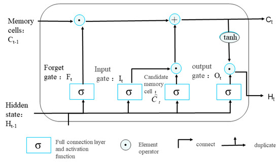
Figure 1.
Neuron structure of LSTM model.
In the above equation, represents the GNSS/PWV time series data, and represent the vector states of the input gate, oblivion gate, and output gate at time t, respectively. represents the sigmoid function; represents the input value at time t with dimensions [n, d] (the number of samples is n, and each sample feature number is shown by the d matrix); is the hyperbolic tangent activation function; is the corresponding weight coefficient matrix and bias term, respectively; is the state of the memory cell at moment t; represents all outputs of the LSTM network cell at moment t; and is the state information of the previous moment. and are weight parameters, and is the deviation parameter.
The GWO algorithm was inspired by the orderly division of labor in the gray wolf performing pack predation behavior and was proposed by Mirjalili et al. in 2014 [32]. By defining all solutions as wolf groups and the prey as the optimal solution, optimization is carried out by imitating the process used by wolf predators. The GWO algorithm has the advantages of excellent global convergence and a fast optimization speed. In order to obtain the optimal function value, the fitness function of the grey wolf algorithm is set to RMSE, and the LSTM parameters are optimized. This solves the shortcomings of time-consuming manual parameter adjustment and makes it easy to fall into a local optimum, further improving the prediction accuracy.
3. Combination Model and Accuracy Evaluation
In this paper, to effectively extract linear and nonlinear information from GNSS water vapor hourly product data, we used the decomposition analysis combined model to reconstruct the water vapor data. For the decomposition process, we used the CEEMDAN algorithm to decompose the original time series into several subsequences and trend items. The purpose was to reduce the complexity of the data and increase the abundance of the original GNSS/PWV data to reduce the difficulty of data feature extraction. The specific decomposition process is shown in Figure 2. For the decomposition process, the permutation entropy was chosen as a measure to calculate the complexity of the subsequence and divide it into high-frequency tendency components according to the randomness and complexity of the combination. Due to the complex and variable characteristics of the high-frequency part despite its small fluctuations, the ARIMA model was chosen for fitting to preserve the data characteristics while reducing the model training time. However, the combination of the low-frequency part and the trend term retained the main features of the original GNSS/PWV data and was a key step in improving the prediction accuracy. An adequate extraction of low-frequency series data features cannot be achieved using only a single linear prediction model and a nonlinear prediction model.
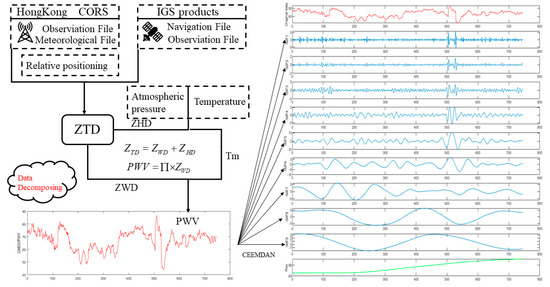
Figure 2.
Data preprocessing process.
Based on the summary and analysis of the current research status of the time series prediction models, this paper proposes a model framework that combines a traditional linear model (ARIMA) and a nonlinear model (LSTM). The main purpose of using the residual method for tandem combination was to decompose the original time series into a linear part and a nonlinear residual part , i.e.,
The modeling steps of the ARIMA–LSTM composite model are as follows:
Step 1: ARIMA is used to complete the modeling and simulation of the data sequence, carry out linear component extraction, and obtain the linear part of the prediction model, denoted as .
Step 2: The fitting residual part of the ARIMA model is solved, and the linear component is extracted from the original sequence to obtain
Step 3: The GWO–LSTM model is used to train the ARIMA modeling residual to obtain the residual prediction value. In the training process, the GWO algorithm is used to optimize the initial weight, threshold, and the number of hidden layer neurons in the LSIM neural network, and the optimal solution of residual is obtained.
Step 4: After solving the linear and nonlinear parts of the predicted values, the two are summed to obtain the final expected value of the low-frequency part of the sequence as
Finally, the ARIMA modeling prediction results of the high-frequency part are summed with the low-frequency prediction results to obtain the full original GNSS/PWV data model prediction results. The specific combination and modeling process are shown in the Figure 3.
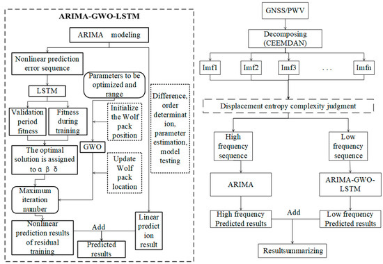
Figure 3.
Workflow of the composite model.
To accurately and objectively reflect the prediction performance of the forecasting model, the root-mean-square error (RMSE), mean squared error (MSE), mean absolute error (MAE), and mean absolute percentage error (MAPE) were used. The model prediction results were evaluated comprehensively.
4. Case Study
4.1. Study Area and Data Description
As a world-class city, Hong Kong has the characteristics of a dense population, an apparent urban heat island, and high coastal humidity. As a result, Hong Kong is prone to the formation of locally severe weather. During the summer, typhoons near the sea are likely to produce considerable rainfall. Thus, it is essential to carry out summer rainfall forecasting. The uniformly distributed CORS system in Hong Kong provides convenience for GNSS/PWV data experiments. The distribution of sites is shown in Figure 4. this study, we selected 18 CORS stations in Hong Kong in July 2021 and used continuous observation data from the LHKS, URUM, CHAN, and TWTF stations in China. The delay phenomenon of GNSS satellite signals in troposphere propagation was quantified to obtain the final PWV data. The PWV data were obtained by first estimating the zenith total delay (ZTD), which mainly consists of the zenith hydrostatic delay (ZHD) and the zenith wet delay (ZWD). The formula is as follows:
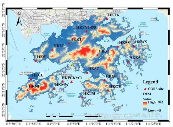
Figure 4.
Distribution of CORS sites in Hong Kong (The bottom picture is labeled in English and Chinese).
The calculated ZWD can be converted to PWV, and the relationship is as follows:
In the formula, ∏ is a dimensionless conversion coefficient; is the liquid water density (1 × 10³ kg/m3); Rw is the water vapor gas constant; and taking 461.495 J/(kg·k) as the refractive index structure constant, K3 = 3.739 ± 0.012 K/hpa, and = 22.13 ± 2.20 K/hpa. Tm is obtained by the Bevis formula (Tm = 0.72Ts + 70.2). The data solution uses GAMIT10.7 to complete the tropospheric delay calculation at the station’s zenith and determines the hourly resolution PWV estimation in mm. The site distribution is as follows:
The plotting of PWV inversion results was completed at 18 stations in the Hong Kong CORS system (Figure 5). It can be intuitively concluded that the trend for water vapor obtained from each station in the region was generally in the same direction. Still, the fluctuations presented in the detailed changes offer the ability to determine the regional microclimate. To verify the correlation between PWV and precipitation, the relationship between GNSS/PWV and actual rainfall was demonstrated by using two groups of CORS stations and weather stations less than 1 km apart: (a) the HKSC station (114°8′28″, 22°19′19″)-Kinsberg weather station (114°10′22″, 22°18′43″) and (b) the HKLM station (114°7′12″, 22°13′8″)-Nanyadao weather station (114°06′31″, 22°13′34″). As shown in Figure 5, heavy rainfall on 23 July was the most representative of the rainfall events that occurred from 1 to 31 July 2021, with a maximum PWV of 82.17 mm at 6.00 on 22 July. When the PWV reached a maximum value of 82.17 mm at 18:00 on 22 July, the PWV began to decline and then started to fall until reaching 45.57 mm at 12:00 on 23 July. The cumulative rainfall recorded at weather stations during this period was 97.1 mm. Therefore, the PWV trend is in good agreement with the actual rainfall situation. Combined with the analysis of rainfall event statistics and meteorological theory knowledge, this shows that there is a gradual increase in PWV before the occurrence of rainfall, followed by a sudden drop in PWV. However, when this phenomenon occurs, it is necessary to consider other meteorological elements and analyze the PWV change rate, change amount, and other factors to accurately predict regional rainfall.
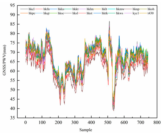
Figure 5.
The overall trend for the PWV data was calculated using data from 18 CORS sites collected in July 2021, Hong Kong.
4.2. Model Forecasting Results
The hourly GNSS water vapor data from 1 to 31 July at the HKCL site were used as a sample totaling 744 data points. The first 720 data points were used as the training set, and the last 24 data points were used as the test set to test the model’s prediction performance. Descriptive statistical analysis was performed on the data, and the results are shown in Table 1, which found that the data had obvious short-term fluctuations and strong randomness. This proves that it is difficult to predict the timing of data accurately.

Table 1.
Descriptive statistics of data.
To cope with the strong randomness of data and obtain better prediction results, we used a predictive model (CEEMDAN–PE–ARIMA–LSTM), the results of which are shown in this section. This prediction model decomposes PWV data from each station into several subcomponents. The combination of ARIMA with the LSTM model was used to predict the subcomponents after recombination. Subsequently, the predicted values for each subcomponent were converted into predicted PWV values by summation. In this paper, the CEEMDAN algorithm was selected to carry out the decomposition of the data, and the decomposition process parameters were set as follows: Adding positive and negative Gaussian white noise standard deviation (Nstd) = 0.2; adding noise number (NR) = 100; maxIter = 500. As shown in Figure 6, the decomposition results showed that the water vapor content in Hong Kong undergoes a gradual upward trend throughout July, which is consistent with the climatic characteristic of a gradual increase in the water vapor content in the air in Hong Kong during the same period leading into summer.
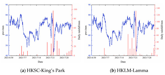
Figure 6.
GNSS/PWV versus measured rainfall at (a) HKSC-King’s Park Meteorological Station and (b) HKLM-Lamma Meteorological Station.
Subsequently, the complexity of each subsequence after decomposition was evaluated using the permutation entropy to achieve a substantial reconstruction of each sequence. The parameters of permutation entropy were set as follows: the embedding dimension of the phase space reconstruction was m = 3, and the delay time was λ = 1. The calculation results are shown in Figure 7. The permutation entropy decreased from imf1 to imf9, and the decreasing rate increased gradually from imf4. By observing the high-frequency feature (imf1–imf4), low-frequency element (imf5–imf9), and trend term (Res) in Figure 8, detailed feature information from the original sequence carried by the high-frequency component was obtained. This intuitively shows the complex changes in the data over the short term and can provide explicit data support for the determination of rainfall, which has little influence on the overall trend. The low-frequency section carries the primary broad pattern information, and the trend term mainly shows the general trend of the data. Therefore, the sequences from imf1 to imf4 were restructured, and the sequences from imf5 to imf9 and the trend term were merged as low-frequency components to form high-frequency components and low-frequency components, respectively. By comparing the low-frequency components with the original GNSS/PWV data, it was concluded that the low-frequency components retain the feature information of the original sequence to the greatest extent. Highly precise predictions are the key to improving the prediction accuracy.
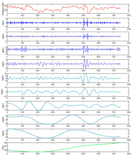
Figure 7.
The PWV decomposition results for CEEMDAN. IMFn represents the nth subcomponent obtained from CEEMDAN. Res indicates the PWV trend after decomposition.
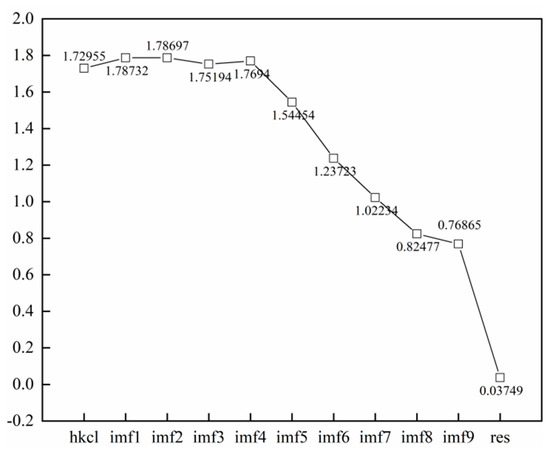
Figure 8.
The permutation entropy of each component.
This study was performed using a combined ARIMA–GWO–LSTM model for the processing of low-frequency components. The specific process used was as follows: First, the unit root (ADF) test was completed for the data, and the second-order difference was used to smooth the data. Then, the model sizing process was completed with the AIC and BIC information criteria, and ARIMA(5,2,5) was derived as the optimal model. Figure 9a shows that the modeling results had a good effect on the linear fitting of data trends during the training process and could be used to complete the linear information extraction of low-frequency components. After modeling, a statistical test of the training residuals showed that the residuals were normally distributed with no first-order correlation. Then, the LSTM model was used to train the residuals.
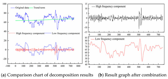
Figure 9.
Reconstructed components: (a) Comparison of the trend terms with the original PWV data and a comparison of the high-frequency and low-frequency components; (b) high-frequency and low-frequency components reconstructed.
The modeling process used for the residual sequence LSTM was as follows: First, normalization was carried out to improve the training efficiency. The Adam algorithm was used to optimize the internal training parameters in the LSTM model structure. The maximum training number was set to 300, the gradient threshold was 1, and the initial learning rate was 0.005. The learning rate was reduced by multiplying the factor by 0.2 after 150 rounds of training. After training, the inverse normalization operation was performed to obtain the residual prediction results. The 24 h prediction results for the single and combined models are shown in Figure 10. It can be seen that the ARIMA model had an excellent linear fitting effect. The prediction results could reflect the overall trend, but the details were poor. By comparing the prediction results of the LSTM and GWO–LSTM models, the LSTM model with its faster convergence and better fitting after parameter search using the gray wolf optimization algorithm had greater prediction accuracy. The single ARIMA, LSTM, and GWO–LSTM models were used for comparison experiments. RMSE, MSE, MAE, and MAPE were used as evaluation indicators for the quantitative analysis. As shown in Table 2, the accuracy indicators were greatly improved. By comparing the experimental results, it was concluded that the combined model has a better prediction effect than using actual observation values, proving that the combined model is more suitable for capturing the characteristics of low-frequency sequence data. Thus, it obtains more precise prediction results.
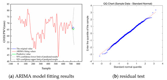
Figure 10.
ARIMA modeling results.
Table 2.
HKCL high-frequency component model prediction accuracy evaluation table.
After completing high-frequency component modeling prediction with ARIMA, the high-frequency component was superimposed on the low-frequency component to obtain the original water vapor data prediction. The final prediction results of each model at the HKCL site were compared with the actual data series in Figure 11. The ARIMA model performed poorly in prediction. The first half of the GWO–LSTM model was not effective, and the second half approached the real number gradually. The overall trend for the GWO–LSTM using CEEMDAN was the same for the decomposition of high- and low-frequency data. Still, there was a significant error in the extreme inflection point, which led to a decrease in the prediction accuracy. The CEEMDAN–ARIMA–GWO–LSTM model adopted in this paper showed better results than the other models in terms of the overall trend and details. The results are shown in Figure 12.
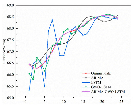
Figure 11.
Comparison of the prediction results obtained with high-frequency component models.
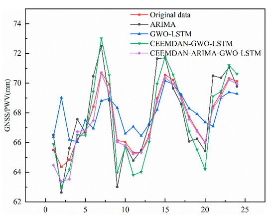
Figure 12.
Comparison of the prediction results for various models.
For the GNSS/PWV data of 18 CORS stations, the prediction accuracy results of single and mixed models are arranged in Table 3. The statistical analysis of the data in the table shows that the LSTM neural network effectively improved the prediction effect of the ARIMA model. The RMSE, MSE, MAE, and MAPE decreased, respectively, by 27.95%, 42.97%, 33.48%, and 34.48% on average; Compared with the mixed model, the RMSE, MSE, MAE, and MAPE of the LSTM neural network were reduced, respectively, by 31.31%, 51.32%, 25.97%, and 27.24% on average, indicating that the mixed model can better obtain the linear and nonlinear data characteristics. This further verifies the prediction performance of the hybrid model.
Table 3.
Model error values of each site.
To visualize the implementation process of the algorithm in this paper, the data of the HKFN site is now used as an example, and Figure 13 is drawn. In view of the uniform distribution of CORS sites in the Hong Kong region combined with the ArcGIS spatial analysis functions, the actual inversion results of PWV and the predicted values of each model for 18 sites in July 2021 are shown. The results of the visual display of the numerical space visualization using kriging interpolation completed at 0:00, 4:00, 8:00, 12:00, 16:00, and 20:00 on July 31 are shown in Figure 14. It can be intuitively concluded that the spatial distribution of water vapor in Hong Kong on a given day gradually increases from west to east and gradually decreases from the coastal area to the inland area. The continuous changes indicate that the water vapor in some regions has a short period of rising and falling. In this regard, a quantitative analysis of regional rainfall should be carried out to determine the connection of water vapor with rain and space.
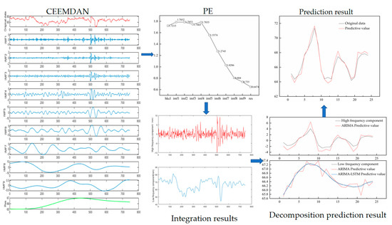
Figure 13.
Data prediction process for the HKFN site.
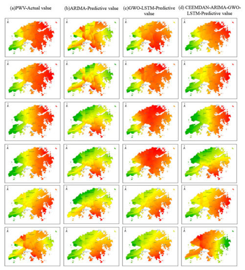
Figure 14.
The results of the visual display of the numerical space visualization using kriging interpolation completed at 0:00, 4:00, 8:00, 12:00, 16:00, and 20:00 on July 31. Where (a) the original data is used, (b) the ARIMA model prediction results are used, (c) the GWO-LSTM model prediction results are used, (d) the combined model prediction results of this paper are used.
5. Discussion
The observation conditions and station density limit the monitoring of the atmospheric water vapor content, and it is difficult to determine the water vapor change in a particular area. With the gradual maturity of GNSS/PWV technology, the construction of CORS systems in various regions has gradually improved. The effective use of CORS stations with uniform spatial distribution and a high continuous resolution can provide scientific data support for rainfall forecasting in small urban areas. The ARIMA model’s data stability greatly affects GNSS/PWV time series. The maximum root-mean-square error is 4.17 mm, and the minimum value is 1.43 mm. The prediction accuracy differs between stations. The overall accuracy of water vapor prediction using LSTM is stable, but there are some limitations, such as a long training time and complex prediction mechanism. Using CEEMDAN, the different scale characteristics of the original sequence are revealed, and the non-stationary data are transformed into static data, which improves the stability and prediction accuracy of the ARIMA model. At the same time, the LSTM model can be used to complete the residual training of the ARIMA model, and the best prediction effect is given according to the model’s advantages. The results of our study show that the accuracy evaluation indexes of the combined model have values that are more than 20% higher than those of single models.
Our experiments show that the decomposition strategy is an effective means to improve the prediction of water vapor. Analyzing the high frequency, low frequency, and trend items after decomposition is helpful for identifying the detailed characteristics of water vapor change. Information on the short-term fluctuations in water vapor from the high-frequency part can be used for rainfall identification and judgment of conditions. The low frequency plus trend part effectively retains the original form of water vapor data and has reduced modeling difficulty and an improved overall prediction accuracy. By combining the influences of regional climate factors and topographic information, it can provide better forecasting conditions for the building of forecasting models, meet requirements for obtaining more accurate digital rainfall warnings, and provide data support for disaster prevention and mitigation work, such as urban waterlogging and mountain natural disaster warnings. This research, however, is subject to several limitations. Firstly, in terms of data selection, data collected in Hong Kong on the first 30 days of July were used as a sample for the last day of prediction, because there is a strong seasonal cycle for water vapor change. July is in the local summer period, and data collected before and after this period have overall similarity. Annual data modeling needs to take into account the four-season cyclical change factors. Secondly, during the process of data interpretation, the overall interpretation of regional CORS data was adopted, and when the monitoring area was larger and more stations were available, it was necessary to group and classify the interpretation of the climate correlation more regionally. In this paper, we studied a whole month of data for Hong Kong after entering the summer season, a strategy which has strong representativeness and research significance. At the same time, based on the single variable time series model prediction research, this paper used the spatial interpolation algorithm to display the prediction results. The geographical spatial factors were not added to the prediction process, and this could be a further optimization direction. Parameter optimization, new model selection, and the training acceleration method also need to be considered.
6. Conclusions
In this study, we used a hybrid model based on CEEMDAN combined with ARIMA and LSTM: the CEEMDAN–PE–ARIMA–GWO–LSTM model. In this model, the original GNSS/PWV data sequence is decomposed by CEEMDAN. The role of PE is to measure the subsequence complexity to classify high-frequency and low-frequency sequences. The ARIMA–GWO–LSTM combined model is used for low-frequency subsequence prediction. ARIMA is used to predict high-frequency subsequences with high complexity to reduce the machine learning training time and combine the prediction results to achieve the prediction task. The regional interpolation task is achieved using the kriging interpolation method for point water vapor values, which analyzes restricted water vapor movement and abrupt changes. The following conclusions were drawn based on the evaluation of the prediction results and the spatial distribution presentation.
- (1)
- The prediction accuracy of the hybrid model is higher than that of the single model. By using the low-frequency component of decomposed data from the HKCL site, ARIMA, LSTM, GWO–LSTM, and ARIMA–GWA–LSTM were used to form a comparative experiment. The results show that the accuracy of the traditional ARIMA model is slightly lower than that of the LSTM neural network. However, it has the advantages of a fast training speed and stable and smooth prediction results. After optimizing the LSTM using the GWO optimization algorithm, each accuracy index was reduced by 78.35% on average. The combined model has better linear and nonlinear information extraction properties and can obtain better prediction results.
- (2)
- CEEMDAN decomposition improved the prediction accuracy compared with a single model for all 18 sets of data validation tests. This indicates that CEEMDAN can reduce the randomness of the original GNSS/PWV data and improve the predictability. It has been proven that optimization means, decomposition methods, and combination strategies can effectively improve the accuracy of CORS water vapor prediction.
- (3)
- By optimizing the GNSS/PWV time series modeling method, more accurate model prediction results can be obtained. This provides data support for regional precipitation prediction and information on the scientific conditions for the formation mechanism and the prediction of small-scale extreme precipitation.
Author Contributions
X.X. designed the algorithm, performed the data processing and analysis, and completed the experimental validation process; W.L., Y.H., F.L. and J.L. contributed to the formation of the logic and structure of the scientific presentation, the interpretation of the results, and the review of the manuscript. All authors have read and agreed to the published version of the manuscript.
Funding
This research was funded by the Anhui Science and Technology Major Project (Grant No. 202103a05020026); Anhui Provincial Natural Science Foundation Project (No. 2008085MD114); Key Research and Development Plan of Anhui Province (No.: 202104a07020014); Anhui Natural Science Foundation Youth Project (No. 2208085QD115); Anhui Provincial Department of Education Natural Science Key Projects (Number: KJ2020A0311) and the National Nature Science Foundation of China (No. 41474026). The authors greatly acknowledge the Department of Earth Atmospheric and Planetary Sciences, MIT, for providing GAMIT/GLOBK software. The authors appreciate the International GNSS Service and Hong Kong Observatory for providing relevant data and products.
Institutional Review Board Statement
Not applicable.
Informed Consent Statement
Not applicable.
Data Availability Statement
Not applicable.
Conflicts of Interest
The authors declare no conflict of interest.
References
- Igor, I.Z.; Richard, P.A. Water vapor variability in the tropics and its links to dynamics and precipitation. J. Geophys. Res. Atmos. 2005, 110, 21112. [Google Scholar]
- Liang, H.; Cao, Y.; Wan, X.; Xu, Z.; Wang, H.; Hu, H. Meteorological applications of precipitable water vapor measurements retrieved by the national GNSS network of China. Geod. Geodyn. 2015, 6, 135–142. [Google Scholar] [CrossRef]
- Dinesh, S.; Jayanta, K.G.; Deepak, K. Precipitable water vapor estimation in India from GPS-derived zenith delays using radiosonde data. Meteorol. Atmos. Phys. 2014, 123, 209–220. [Google Scholar]
- Wu, M.; Jin, S.; Li, Z.; Cao, Y.; Ping, F.; Tang, X. High-Precision GNSS PWV and Its Variation Characteristics in China Based on Individual Station Meteorological Data. Remote Sens. 2021, 13, 1296. [Google Scholar] [CrossRef]
- Ying, L.; Gottfried, K.; Barbara, S.; Marc, S.; Johannes, K.N.; Shu-peng, H.; Yun-bin, Y. A New Algorithm for the Retrieval of Atmospheric Profiles from GNSS Radio Occultation Data in Moist Air and Comparison to 1DVar Retrievals. Remote Sens. 2019, 11, 2729. [Google Scholar]
- YAO, Y.; Zhang, S.; Kong, J. Research Progress and Prospect of GNSS Space Environment Science. Acta Geod. Cartogr. Sin. 2017, 10, 1408–1420. [Google Scholar]
- SHEN, Y.-Z. Study of Recovering Gravitational Potential Model from the Ephemeredes of CHAMP; Institute of Geodesy and Geophysics, Chinese Academy of Sciences: Wuhan, China, 2000. [Google Scholar]
- Biyan, C.; Zhizhao, L.; Wai-Kin, W.; Wang-Chun, W. Detecting Water Vapor Variability during Heavy Precipitation Events in Hong Kong Using the GPS Tomographic Technique. J. Atmos. Ocean. Technol. 2017, 34, 1001–1019. [Google Scholar]
- Ping-Wah, L.; Wai-Kin, W.; Ping, C.; Hon-Yin, Y. An overview of nowcasting development, applications, and services in the Hong Kong Observatory. J. Meteorol. Res. 2014, 28, 859–876. [Google Scholar]
- Qingzhi, Z.; Xiongwei, M.; Yibin, Y. Preliminary result of capturing the signature of heavy rainfall events using the 2-d-/4-d water vapour information derived from GNSS measurement in Hong Kong. Adv. Space Res. 2020, 66, 1537–1550. [Google Scholar]
- Dong, S.; Xing, Z.; Lou, D.; Zhang, Y.; Zhang, H.; Guo, H. Short-term rainfall forecasting based on a modified RBF function. J. Shenyang Agric. Univ. 2017, 3, 367–372. [Google Scholar]
- Ge, Y.H.; Xiong, Y.L.; Chen, Z.S.; Chen, H.B.; Long, J.L. Prediction method of GPS precipitation based on wavelet neural network. Sci Surv. Mapp. 2015, 9, 28–32. [Google Scholar]
- Shengwei, W.; Juan, F.; Gang, L. Application of seasonal time series model in the precipitation forecast. Math. Comput. Model. 2013, 58, 677–683. [Google Scholar]
- Şenkal, O.; Yıldız, B.Y.; Şahin, M.; Pestemalcı, V. Precipitable water modelling using artificial neural network in Çukurova region. Environ. Monit. Assess. 2012, 184, 141–147. [Google Scholar] [CrossRef]
- Vázquez B, G.E.; Grejner-Brzezinska, D.A. GPS-PWV estimation and validation with radiosonde data and numerical weather prediction model in Antarctica. GPS Solut. 2013, 17, 29–39. [Google Scholar] [CrossRef]
- Yingchun, Y.; Tao, Y. Predicting precipitable water vapor by using ANN from GPS ZTD data at Antarctic Zhongshan Station. J. Atmos. Sol. Terr. Phys. 2019, 191, 105059. [Google Scholar]
- Sharifi, M.A.; Souri, A.H. A hybrid LS-HE and LS-SVM model to predict time series of precipitable water vapor derived from GPS measurements. Arab. J. Geosci. 2015, 8, 7257–7272. [Google Scholar] [CrossRef]
- Chien-Ming, C. Wavelet-Based Multi-Scale Entropy Analysis of Complex Rainfall Time Series. Entropy 2011, 13, 241–253. [Google Scholar]
- Wang, W.; Yujin, D.; Chau, K.; Chen, H.; Liu, C.; Ma, Q. A Comparison of BPNN, GMDH, and ARIMA for Monthly Rainfall Forecasting Based on Wavelet Packet Decomposition. Water 2021, 13, 2871. [Google Scholar] [CrossRef]
- Wang, H.; Wang, W.; Du Yujin; Xu, D. Examining the Applicability of Wavelet Packet Decomposition on Different Forecasting Models in Annual Rainfall Prediction. Water 2021, 13, 1997. [Google Scholar] [CrossRef]
- Niu, M.; Wang, Y.; Sun, S.; Li, Y. A novel hybrid decomposition-and-ensemble model based on CEEMD and GWO for short-term PM 2.5 concentration forecasting. Atmos. Environ. 2016, 134, 168–180. [Google Scholar] [CrossRef]
- Qi, O.; Wenxi, L.; Xin, X.; Yu, Z.; Weiguo, C.; Ting, Y. Monthly Rainfall Forecasting Using EEMD-SVR Based on Phase-Space Reconstruction. Water Resour. Manag. 2016, 30, 2311–2325. [Google Scholar]
- Yang, Z.; Zou, L.; Xia, J.; Qiao, Y.; Cai, D. Inner Dynamic Detection and Prediction of Water Quality Based on CEEMDAN and GA-SVM Models. Remote Sens. 2022, 14, 1714. [Google Scholar] [CrossRef]
- Yuan, R.; Cai, S.; Liao, W.; Lei, X.; Zhang, Y.; Yin, Z.; Ding, G.; Wang, J.; Xu, Y. Daily Runoff Forecasting Using Ensemble Empirical Mode Decomposition and Long Short-Term Memory. Front. Earth Sci. 2021, 9, 621780. [Google Scholar] [CrossRef]
- Zhang, J.; Tang, H.; Tannant, D.D.; Lin, C.; Xia, D.; Liu, X.; Zhang, Y.; Ma, J. Combined forecasting model with CEEMD-LCSS reconstruction and the ABC-SVR method for landslide displacement prediction. J. Clean. Prod. 2021, 293, 126205. [Google Scholar] [CrossRef]
- Ping, L.Y.; Wang, Y.; Wang, Z. RBF prediction model based on EMD for forecasting GPS precipitable water vapor and annual precipitation. Adv. Mater. Res. 2013, 765, 2830–2834. [Google Scholar]
- Flandrin, P.; Rilling, G.; Goncalves, P. Empirical mode decomposition as a filter bank. IEEE Signal Proc. Let. 2004, 11, 112–114. [Google Scholar] [CrossRef]
- Torres, M.E.; Colominas, M.A.; Schlotthauer, G.; Flandrin, P. A complete ensemble empirical mode decomposition with adaptive noise. In Proceedings of the 2011 IEEE International Conference on Acoustics, Speech and Signal Processing (ICASSP), Prague, Czech Republic, 22–27 May 2011; pp. 4144–4147. [Google Scholar]
- Bandt, C.; Pompe, B. Permutation entropy: A natural complexity measure for time series. Phys. Rev. Lett. 2002, 88, 174102. [Google Scholar] [CrossRef] [PubMed]
- Shannon, C.E. A mathematical theory of communication. Bell Syst. Tech. J. 1948, 27, 379–423. [Google Scholar] [CrossRef]
- Hochreiter, S.; Schmidhuber, J. Long Short-Term Memory. Neural Comput. 1997, 9, 1735–1780. [Google Scholar] [CrossRef]
- Mirjalili, S.; Mirjalili, S.M.; Lewis, A. Grey Wolf Optimizer. Adv. Eng. Softw. 2014, 69, 46–61. [Google Scholar] [CrossRef] [Green Version]
Publisher’s Note: MDPI stays neutral with regard to jurisdictional claims in published maps and institutional affiliations. |
© 2022 by the authors. Licensee MDPI, Basel, Switzerland. This article is an open access article distributed under the terms and conditions of the Creative Commons Attribution (CC BY) license (https://creativecommons.org/licenses/by/4.0/).