Abstract
Understanding the response of tropospheric ozone (O3) to nitrogen dioxide (NO2) change is important for local O3 control. The relationship between O3 and NO2 at county scale in China has been extensively studied using models, but there is a lack of results from direct measurements. In this study, we used measurements of O3, NO2 and meteorological conditions from a dense network in the Yangtze River Delta (YRD), and satellite observed formaldehyde (HCHO) and NO2 column densities for the analysis of O3 variabilities and its relationship to NO2. As a result, severe O3 pollution occurred mainly in Shanghai city, southern Jiangsu and northern Zhejiang provinces in YRD during April–September. In addition, meteorological conditions could explain 54% the diurnal O3 variation over YRD. During April–September 2015–2021, O3 showed a significant positive relationship (r = 0.61 ± 0.10) with NO2 after removing the impact from meteorological conditions. However, the relationship could be reversed with NO2 concentration change. Our result suggested that the controllable O3 related to NO2 change is up to 100 μg·m−3 in megacities over Shanghai and northern Zhejiang province. The O3 is much more sensitive to the NO2 reduction in megacities than surrounding areas. Our results evaluate the different impacts of NO2 changes on O3 formation, which provides explanation for the simultaneously alleviated O3 pollution and reduced NO2 in 2020 in Shanghai and northern Zhejiang, as well as the increased O3 in most counties before 2019 with reduced NO2 during October–March. The driving mechanism as revealed from this study for O3 and NO2 will be valuable for the O3 abatement through NO2 reduction at sub-county scale over YRD in China.
1. Introduction
Tropospheric ozone (O3), an important greenhouse gas and secondary air pollutant in the atmosphere, is harmful to human health and terrestrial ecosystems [1,2,3]. Because of its damage to plant tissue and the sharp drop in crop and wood production, it deserves attention from farmers, scientists and the public [4]. In the Yangtze River Delta (YRD) of eastern China, this kind of concern is increasing [5], because it continues to increase despite a series of clean-air regulations since 2013. As we know, tropospheric O3 is mainly formed through complicated photochemical reactions of volatile organic compounds (VOCs) and nitrogen oxides (NOx) [6]. The large-scale surface extreme ozone pollution in YRD could also be aggravated by local production, downward and regional transport aggravated [7]. The more complex driving mechanisms of O3 formation, compared with those of primary pollutants from anthropogenic emissions for the mixed impacts from meteorological conditions and the precursor proportion variation [8], limit the effectiveness of O3 abatement strategies. Therefore, understanding the spatio-temporal variation of O3 pollution, its relationship to the meteorological conditions and its precursors’ variation is important for O3 abatement plan.
Meteorological conditions (such as relative humility (RH), air temperature (AT) and sunshine duration (SD), etc.), through affecting the chemical reaction rates, emission rates (e.g., biogenic VOCs) and precursors deposition (e.g., NOx dissolved in precipitation), become important factors for ground-level O3 formation [9,10]. Due to its regional variability, the meteorological effect on O3 pollution should be considered in different regions [11]. For example, the dominant meteorological factors for northern, eastern and southern China are AT, SD and RH, respectively [8]. In YRD, the co-pollution of O3 was found to occur under meteorological conditions of strong radiation, higher surface air temperature and lower wind speed [12,13]. As a result, understanding the relationship between O3 and its precursors, after removing the meteorological effects, is important to come up with measures for alleviating the O3 pollution [6].
The increased anthropogenic emissions of O3 precursors are the primary sources of tropospheric O3 pollution [14]. Therefore, reducing human-emitted NOx and VOCs is a crucial process for O3 abatement [15]. However, ground-level O3 response to its precursor variation was found to be nonlinear, complicated by a series of photochemical reactions [16]. According to the sensitivity of O3 to its precursors, the photochemical regime can be divided into three categories: VOC-limited, NOx-limited and mixed sensitive [17]. It indicates that the effectiveness of O3 control may require the reduction of different precursors’ emissions. It was also found that emission reduction with reasonable control ratios of NOx and VOCs were effective for decreasing both PM2.5 and O3 in the YRD [18]. Moreover, the photochemical regime could vary with the ratio of NOx and VOCs in the atmosphere, which changes in time and space [19]. In addition to anthropogenic emissions, biogenic VOCs (BVOCs) could also be important O3 precursors within the cities [20]. Therefore, it is of great significance to understand the sensitivity of O3 to its precursor substances at a finer scale for the effective prevention of O3 pollution [21]. However, the controllable amounts of O3 to its precursor’s reduction and its sensitivity to the precursors change at county-scale are still unclear especially over the YRD, where dense urban agglomeration is located.
The changing meteorological conditions and the distribution of NOx related to different human activities have significant effects on the spatial heterogeneity of O3 pollution. Previous studies of ground-level O3 pollution in China mainly used the data from national ambient stations [8,22], which are sparse and unevenly distributed in space and therefore limits a finer analysis of O3 pollution and its causes. A larger number of regional sites for monitoring O3 could provide more information for understanding the local O3 variations and the driving mechanism of its response to the change of meteorological conditions and precursor emissions [23]. In this study, we aim to use measurements of O3, NO2 and the meteorological conditions from a dense network over YRD, combined with satellite observations, for understanding O3 abatement strategies through the analysis of O3 variabilities and its relationship with meteorological conditions and ground-level NO2.
2. Materials and Methods
2.1. Study Area
The Yangtze River Delta (YRD), including the city of Shanghai, and the provinces of Jiangsu, Zhejiang and Anhui in eastern China, is one of the largest urban agglomeration in the world (Figure 1). It belongs to a humid subtropical climate zone, which is characterized by hot, humid summers, and cool to mild winters. O3 pollution occurred repeatedly mainly in the warm season (April–September) over the past several years [15]. There are several megacities with more than 9.0 million residents in YRD, which contribute significantly to the anthropogenic emissions of O3 precursors [24].
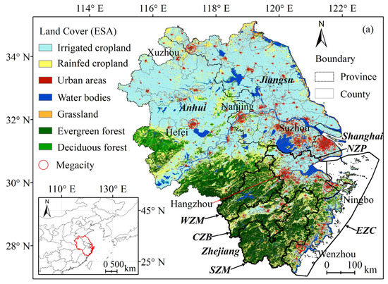
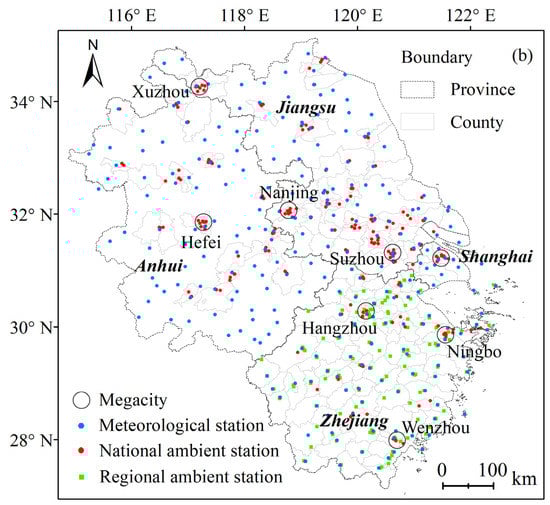
Figure 1.
(a) Geographical map and land cover, (b) dense network of ambient and meteorological stations over the Yangtze River Delta used in this study. Megacities with residents more than 9.0 million in 2021 are shown with a red/black circle. Selected regions of different land cover are highlighted with black lines (a). Regional ambient stations for O3 measurements are mainly distributed in Zhejiang province (b).
In order to better understand the spatial difference of O3 pollution, regions of different geography over the Zhejiang province are also divided and selected for the regional O3 variation analysis. Those include Northern Zhejiang Plain (NZP), Western Zhejiang Mountain (WZM), Central Zhejiang Basin (CZB), Southern Zhejiang Mountain (SZM) and Eastern Zhejiang Coast (EZC) (Figure 1a). The main land cover in these regions is different, which indicates that different human and natural activities affect the O3 formation.
2.2. The Dense Network for Measuring Ground-Level O3, Its Precursors and Meteorological Conditions
Hourly O3, its precursors and meteorological conditions from 2015 to 2021 are measured by dense network shown in Figure 1b. The significance of the dense network is twofold: (1) It includes both 252 meteorological stations (blue points) and 412 ambient stations (red and green points); (2) There are not only normally used national but also 196 regional ambient stations. The increased measurements from regional ambient stations make it possible for the O3 pollution analysis on a county scale. The data quality control for the monitoring was carried out according to the national standard HJ/T193-2013. Furthermore, invalid observations with missing measurements were screened before analysis to ensure high data quality for all data pairs. We used all valid measurements from the dense network for the analysis of O3 variabilities and its relationship to meteorological conditions and precursors over the YRD. An 8 h running average was applied to the hourly O3 measurements. Daily maximum 8 h average (MDA8) value was used for comparison with China’s air quality standard for O3: 160 μg·m−3 [25]. The maximum value of all sites’ measurements inside each county, and the mean value of all counties’ maximum value are adopted for the evaluation at county or local scales, respectively. Hourly NO2, an effective proxy for NOx, in each station was used for the precursor analysis.
Hourly meteorological measurements were also archived by the Zhejiang Meteorological Bureau and used in this study. The distribution of national meteorological stations is shown in Figure 1b. Sunshine duration (SD), 2 m air temperature (AT) and relative humidity (RH) from 2015–2021 were used. For each O3 observation station, the meteorological data nearest to the station were collected.
2.3. Ozone’s Precursors Observed by TROPOMI
TROPOMI is a hyperspectral nadir-viewing imager aboard the Sentinel-5 Precursor (S5P) satellite that was launched on 13 October 2017 by European Space Agency (van Geffen et al., 2020). It observes various air pollutants at 13:30 local time each day with a high spatial resolution of 7 × 3.5 km2 (5.5 × 3.5 km2 after 6 August 2019). Tropospheric formaldehyde (HCHO) and nitrogen dioxide (NO2) column densities, which are proxies for VOCs and NOx, respectively, observed by TROPOMI from 1 June 2018 to 31 December 2021 were used for the analysis of O3 sensitivity to precursors [26] in this study. Good quality (qa_value > 0.75) data were collected after filtration of cloud scenes, errors and problems [27]. Daily HCHO and NO2, collected from google earth engine [28] and resampled to 3.5 × 3.5 km, were used for the sensitivity analysis of O3 to its precursor’s reduction in this study.
2.4. Driving Mechanism Analysis of Meteorological Conditions and Ozone’s Precursors
The method of moving window average was used for calculating the diurnal variation of SD/AT/RH. In addition, we divided daily O3 concentration to be 32 levels (<30, 30–32, …, 178–180, >180 μg·m−3), and the corresponding SD/AT/RH in each level were averaged. In the driving analysis, we made a series of correlation and regression analysis. Firstly, we use the Spearman Rank correlation method and t-test to analyze the correlation between ozone and meteorological conditions. Before the correlation analysis, we tested the normal distribution of datasets. Secondly, according to the related results, single/multiple linear regression analysis between O3 and the meteorological conditions were conducted. Thirdly, O3 residuals (ΔO3), which are obtained by subtracting the multiple linear regression results from daily ground-level O3, were used for correlation analysis with the precursor. The F-test and t-test were used for significant testing for the multiple linear regression and fitted coefficients, respectively.
Ground-level NO2, one of the most important anthropogenic emissions of O3 precursors, was used for the driving mechanism analysis. First, Pearson correlation coefficient and t-test were used for identifying the relationship between ΔO3 and NO2. Second, regressions of linear, exponential and logarithmic functions, were applied to ΔO3 and NO2, separately. The root mean square error (RMSE) and coefficient of determination (R2) were used for evaluating the fitting reliability. Third, the optimal fitting would be used for calculating the controllable amount of O3 and its variation gradient related to the NO2 reduction. In the end, we present the O3 variations and gradient response to NO2 change at sub-county scale in YRD.
2.5. Sensitivity Analysis of Ozone to Its Precursor’s Reduction
Satellite observed HCHO/NO2 ratios (HNR, <1.0, 1.0–2.0 and >2.0) were widely used for identifying the VOC-limited, NOx-limited and mixed sensitive regimes in previous studies [29]. In particular, the ΔO3 might show significantly positive/negative relation with the NO2 in the driving mechanism analysis over some megacities. The relationship varies with the O3 formation condition of meteorology and precursors change at local scales. In this study, the TROPOMI observed daily HNR in each ambient station was used for the sensitivity analysis.
First, data pairs of ground-level ΔO3 and NO2 at 13:00 to 14:00 local time, and the corresponding HNR during the April–September and October–March was classified. Second, an initial threshold of HNR was then generated from 1.0 to 5.0 for April–September and 2 to 0 for October–March with a setting gradient (0.01 here). The Pearson correlation coefficient (r) and t-test (p) was calculated using data pairs of ΔO3 and NO2 in different part as separated by the threshold. Third, the opposite relevance and significance in different part would be used for screening the threshold. The discriminant conditions of r > 0.2 and p < 0.05, indicating significant correlation, were applied here. In the end, the threshold was generated for each city or county, and compared with satellite observed daily HNR for the O3 abatement plan from NO2 reduction.
3. Results and Discussion
3.1. Sub-County Scale Ozone Pollution from the Dense Measurements
During 2015–2021, megacities in YRD, especially for regions of Shanghai, northern Zhejiang and southern Jiangsu provinces, suffered high O3 pollution (exceeding the threshold of 160 μg·m−3) for more than 36 days per year (Figure 2a). Counties in southern Zhejiang and Anhui provinces were less affected by O3 pollution. In 2020, with emissions reduction due to COVID-19 [30], O3 pollution was relieved in most counties, especially for those in northern Zhejiang and Shanghai (Figure 2b), but it remained severe in some counties of southern Jiangsu province.
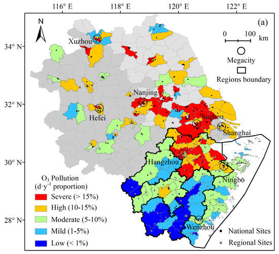
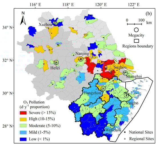
Figure 2.
Spatial distribution of O3 pollution in (a) 2015–2021 and (b) 2020 over each county generated with the measurements from the dense ambient stations over the Yangtze River Delta. Megacities with residents more than 9.0 million in 2021 shown with black circle. The separated regions of Zhejiang province are highlighted with black lines.
The spatial connectivity of the mitigation and presence of O3 pollution could be affected by atmospheric transportation. Although O3 is a short-lived trace gas, typically hours in polluted urban regions, its lifetime in the free troposphere is of the order of several weeks [31], sufficiently long for it to be transported over regional scales [32]. As a results, O3 variation is still partly driven by horizontal and vertical atmospheric transport. In addition, O3 precursors could be transported over megacities in YRD, which could affect the local O3 variation [33]. Atmospheric transported anthropogenic and biogenic emissions of VOCs could partly contribute to the O3 enhancement of megacities over YRD during April–September. It was found that plenty of BVOCs molecules could be transported from the county of Fuyang in Zhejiang to Shanghai, which resulted in the gradual rise of O3 in Shanghai [5]. In addition, local O3 could also be affected by the transported air from the nearby upwind areas [15]. Model simulations also showed that atmospheric transport can regulate the regional interactions of ozone pollution in China, and YRD can export large amounts of ozone to the surrounding areas [34]. That supports the results that some counties with little precursor emissions in YRD show similar pollution and mitigation as megacities nearby.
In this temporal variation analysis (Figure 3), we selected four capital cities of provinces in YRD and the selected regions (Figure 1a) of Zhejiang province as case studies. In megacities or urban regions, O3 concentration could vary from 50 μg·m−3 in winter to more than 100 μg·m−3 in summer, and high O3 concentration and pollution were mainly concentrated in April–September. The pollution days in April–September are 8.11 ± 2.05/1.59 ± 1.32 d·mon−1 in megacities/regions, which is more than 8 times that in October–March (0.66 ± 0.41/0.18 ± 0.16 d·mon−1). O3 pollution occurred mainly before 2019 and dropped sharply in 2020, with a drop of 40.43% in megacities (from 9.22 ± 2.45 d·mon−1 in 2019 to 5.49 ± 1.12 d·mon−1 in 2020). This kind of sharp change of O3 could be related to COVID-caused emissions reduction [35]. However, there are also some differences in the variations, such as the decrease of O3 concentration in Hangzhou/NZP during April–September but increase in October–March. There is a possibility that NO2 reduction could promote the O3 enhancement during winter time [36]. As a result, understanding the driving mechanism of O3 formation is important for interpreting these different variations in space and time as described above. Although O3 is a short-lived trace gas, typically hours in polluted urban regions, its lifetime in the free troposphere is of the order of several weeks [31], sufficiently long for it to be transported over regional scales [32]. As a result, O3 variation is still partly driven by horizontal and vertical atmospheric transport. Just like the spatial connect of O3 pollution (Figure 2) and O3 precursor’s ratios, O3 precursors could be transported over megacities in YRD, which could affect the local O3 variation [33]. Atmospheric transported anthropogenic and biogenic emissions of VOCs could partly contribute to the O3 enhancement of megacities over YRD during April–September. It was found that plenty of BVOCs molecules could be transported from the county of Fuyang in Zhejiang to Shanghai, which resulted in the gradual rise of O3 in Shanghai [5]. In addition, local O3 could also be affected by the transported air from the nearby upwind areas [15]. Model simulations also showed that atmospheric transport can regulate the regional interactions of ozone pollution in China, and YRD can export large amounts of ozone to the surrounding areas [34]. That supports the results that some counties with little precursor emissions in YRD show similar pollution and mitigation as megacities nearby. However, quantitative research of the contribution from atmospheric transportation to O3 pollution over the YRD needs further study.
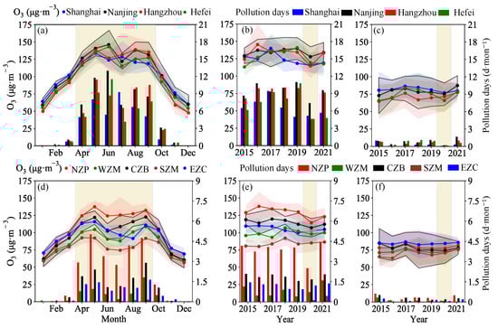
Figure 3.
Megacities’ and regional monthly variation (a,d) from 2015 to 2021, and yearly variation during (b,e) April–September and (c,f) October–March of mean O3 concentration and pollution days per month. One standard deviation of O3 concentration is shown as a shadow of the corresponding color. Regions of NZP, WZM, CZB, SZM and EZC were divided in Section 2.1 and Figure 1.
3.2. Driving Mechanism Analysis of O3 Variation with Meteorological Conditions and Ground-Level NO2
For all megacities, the daily variation of ground-level O3 shows a significant positive correlation with AT and SD, and negative correlation with RH (Figure 4). It also shows that the O3 variation that affected by the rainy season has a pattern of rise-fall-rise (Figure A1). Results from multiple linear regression (Table 1) show that the AT, RH and SD could explain up to 54% of the diurnal O3 variation over these capital cities (R2 = 0.54 ± 0.09, Sig-F < 0.01), which is higher than single of temperature (40%) as shown in Liu et al. [8]. The contribution from SD and AT is similar (3.44 ± 1.09 and 2.98 ± 0.21), which is significantly stronger than that of RH (−0.79 ± 0.19).
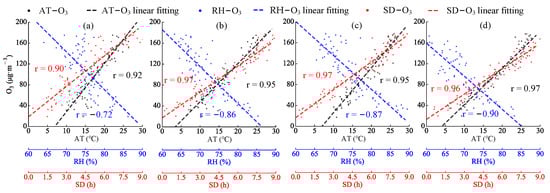
Figure 4.
Relationship between various levels of daily O3 and air temperature (AT: black), sunshine duration (SD: red) or relative humility (RH: blue) over four capital cities (a) Shanghai, (b) Nanjing, (c) Hangzhou, (d) Hefei in the Yangtze River Delta.

Table 1.
Statistics of multiple linear regression for daily O3 and meteorological conditions.
O3 residuals (ΔO3), related to the impact from its precursors [6], could be derived by removing the fitting result from multiple regression with meteorological conditions. During April–September, ΔO3 is significantly positive correlated with NO2 variation (0.62 ± 0.12) in the four capital cities (Figure 5a–d and Table 2), which indicates the effectiveness of NO2 reduction to the O3 abatement. However, the correlation is different, with significant negative in Hangzhou and Nanjing, positive in Shanghai and no correlation in Hefei, during October–March (Figure 5e–h). These could give some explanation for the sharp decrease of O3 during April–September but increase during October–March in 2020 [37]. It also shows the different sensitivity in different time and space.
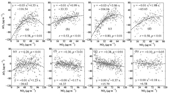
Figure 5.
Data pairs of ΔO3 and NO2 concentration during (a–d) April–September and (e–h) October–March over four capital cities (a,e): Shanghai; (b,f): Nanjing; (c,g): Hangzhou; (d,h): Hefei in the Yangtze River Delta. ΔO3 is ozone concentration after removing the fitting results from multiple linear regression with meteorological conditions.
Table 2.
Statistics of the relationship, multiple regression of linear, exponential and logarithmic functions between ΔO3 and NO2, and the controllable O3 related to NO2 adjustment.
The change of the correlation between ΔO3 and NO2, which indicates the different effectiveness of NO2 reduction to O3 control, is critical for the design of effective O3 abatement plan [38]. Firstly, the correlation could be significantly different during April–September and October–March in some megacities, which is consistent with differences in the control of major precursors during different periods [39]. Secondly, the correlation between ΔO3 and NO2 could reverse with the NO2 increase during April–September (Figure 5), which may indicate the NOx-limited regime could change with precursor ratios changing as shown in previous studies [29]. Thirdly, in the exponential fitting between ΔO3 and NO2 during April–September, the NO2 concentration causing the relationship reverse over these capital cities is different. That could be caused by the different background proportion of O3 precursors over these cities [40]. Fourthly, during October–March, the correlation usually cannot be reversed with NO2 change, which partly supports the result that most cities seem to be VOC-limited regime [41]. That is also can be explained with the decisive effect from the high NOx and low VOCs over the period (Figure A2a). Finally, the O3 concentration enhancement during COVID-19 for the NOx reduction during winter period has been widely researched [30,36], but the benefits from NOx reduction on O3 abatement during April–September were not discussed adequately before. Therefore, the correlation between ΔO3 and NO2 and its change during April–September should be paid more attention and studied further.
According to the ΔO3-NO2 variation shown in Figure 5 and statistics in Table 2, the correlation between ΔO3 and NO2 does not seem to be totally linear. The exponential function fitting, with mean RMSE of 20.71 and R2 of 0.26, is better than that of linear and logarithmic function. The exponential fitting line applied in this study is also shown in Figure 5. Results show that the correlation could be reversed with NO2 increase. It could be caused by the proportion change in precursors with NO2 variation. In addition, we define the differences between the highest and lowest values from the fitted ΔO3 with NO2 variation as the controllable O3 related to the NO2 change. This controllable O3 is significantly different in time and space, which could vary from 6.70 μg·m−3 in Hefei during October–March to 96.31 μg·m−3 in Hangzhou during April–September. The controllable O3 is much larger during April–September (70.64 ± 25.46 μg·m−3) compared with that in October–March (22.36 ± 11.77 μg·m−3).
The controllable O3 could be approaching 100 μg·m−3 during April–September over some counties in Shanghai, Hangzhou and Ningbo cities, which is much larger than that during October–March (Figure 6). This clearly suggests that the O3 abatement strategies should be mainly conducted during April–September in almost of these counties. During April–September, the most controllable area is mainly distributed in counties over Shanghai, the northern Zhejiang plain, and the eastern Zhejiang coast, especially for the cities of Shanghai, Hangzhou, Ningbo and Wenzhou. Differences exist when compared with the O3 pollution shown in Figure 2a where there are some counties with severe O3 pollution but with weak controllable O3 related to NO2 changes, such as those around Suzhou and Nanjing. Those counties were also found to not be significantly alleviated in 2020 (Figure 2b) [38]. These results indicate that the severe O3 pollution in regions with high controllable O3 might be easier to be alleviated. However, the control strategies for the remaining regions will need further study.
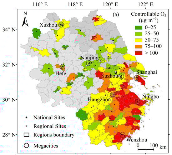
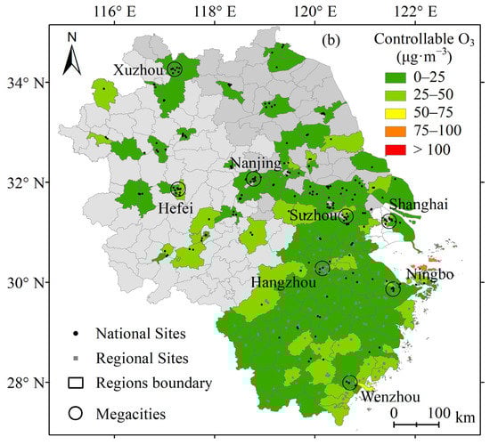
Figure 6.
Controllable O3 related to NO2 adjustment during (a) April–September and (b) October–March in sub-county scale over the Yangtze River Delta.
3.3. Sensitivity of the O3 to NO2 Reduction Inferred from Dense Measurements and Satellite Observations
HCHO/NO2 ratio (HNR) thresholds from Sentinel-5P of the capital cities could be extracted by the sensitivity analysis method (Section 2.5) as shown in Figure 7. Thresholds varies in different periods and cities, which indicate that the sensitivity of O3 related to NO2 reduction varies with the proportion change in precursors. The HNR threshold of NO2 during April–September ranges from 1.45 to 2.85 for the selected capital cities, which is consistent with the threshold of 2.0 for NOx-limited regime in previous studies [5]. However, the sensitivity varies during October–March, with positive correlation in Shanghai and negative correlation in Hangzhou and Hefei. Thresholds of significant negative correlation in Hangzhou and Nanjing is 0.65 and 0.85, which is lower than the threshold of 1.0 for VOC-limited regime.
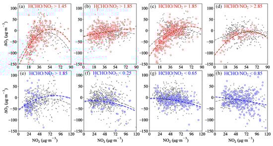
Figure 7.
Separation for the relationship between ΔO3 and NO2 concentration by HCHO/NO2 ratio (HNR) from Sentinel-5P measurements during April–September (top panel) and October–March (bottom panel) over four capital cities (a,e) Shanghai; (b,f) Nanjing; (c,g) Hangzhou; (d,h) Hefei in the Yangtze River Delta.
Amplitudes of atmospheric NO2 and O3 are different in these megacities, which contributes to the different ΔO3 gradient. During April–September, the gradient of ΔO3/NO2 is −0.006 x+ 0.65 in Nanjing and −0.111 x+ 6.17 in Shanghai with 38.73 ± 34.63 and 36.35 ± 30.06 μg·m−3 being the NO2 change, respectively (Table 3). Therefore, it could be more efficient for O3 pollution mitigation in Shanghai than Nanjing with similar NO2 reduction. In addition, the relationship between ΔO3 and NO2 could be reversed with the change of local NO2 concentration, and the critical values of NO2 leading to the change could range from 55.73 (Shanghai) to 107.48 (Nanjing) μg·m−3. Compared to the NO2 range, it could be the reverse in Shanghai, Hangzhou and Hefei, but not in Nanjing. The positive correlation could explain more than (85.9 ± 14.0) % of the NO2 variation for these capital cities. During October–March, the main correlation could be negative in these capital cities, and that could explain (71.1 ± 40.5) % of the NO2 variation.
Table 3.
HCHO/NO2 ratio (HNR) thresholds, relationships between ΔO3 and NO2 (μg·m−3) and ΔO3 variation rate to NO2 change with measurements from the dense network and Sentinel-5P observations over four capital cities in the Yangtze River Delta.
During the main pollution period (April–September), the HCHO/NO2 ratio (HNR) thresholds in megacities are usually lower than surrounding areas (Figure 8a). That could be related to the high NO2 concentration caused by high emissions from intensive human activities such as traffic [8]. Compared with land cover in Figure 1a, values of satellite observed HNR were high in city and plain, and low in mountain areas (Figure 8b). According to the results from Figure 8a,b, NO2 reduction could be available for the O3 mitigation in most areas except for some intermediate zones such as Suzhou city. This result is consistent with the COVID-19 caused O3 variation in 2020 when the NO2 reduction contributes to the significant decrease in cities of Shanghai and Hangzhou but not in Suzhou. Therefore, the sub-county scale HNR sensitivity and satellite observed HNR could provide important implications for the O3 abatement plan through the reduction of NO2.
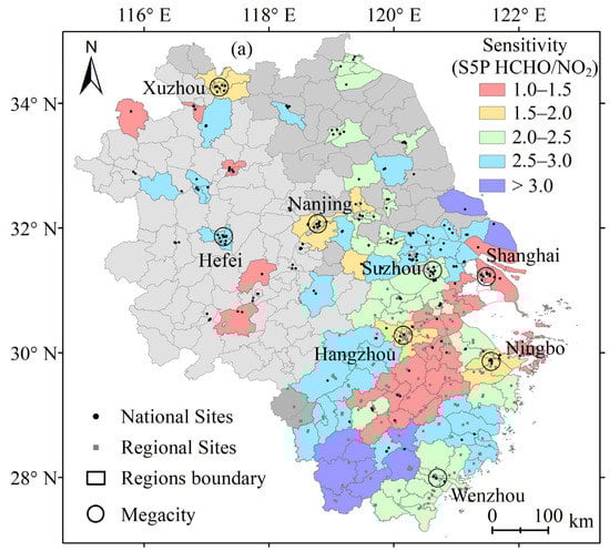
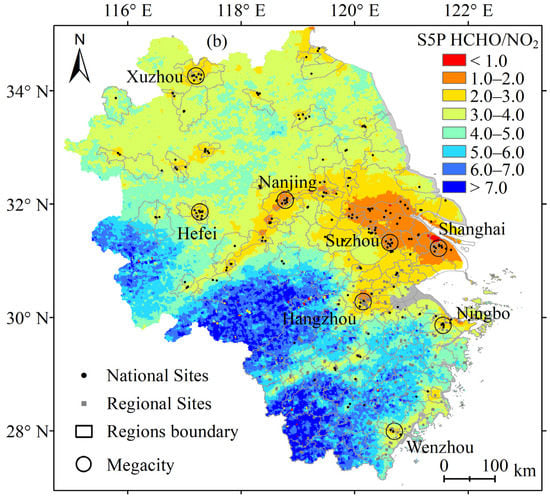
Figure 8.
(a) Sub-county scale HCHO/NO2 ratio (HNR) thresholds from dense measurements and (b) Sentinel 5P observed mean values of HNR during April–September over YRD.
Satellite-observed HNR was widely used for the sensitivity analysis of the response of O3 to its precursor’s variation [38,42]. The sensitivity differences shown in this study are consistent with results from previous studies that NOx-limited regimes dominate in most regions and VOC-limited regimes are distributed in some urban and suburban areas [38,43]. Thresholds of HNR mainly range from 1.0 to 3.0 during April–September and lower than 1.0 during October to March, indicating NOx-limited and VOC-limited regimes, respectively, which is consistent with the sensitivity results before [29]. The different gradient of ΔO3/NO2 over these cities during April–September contributing to the different benefits of O3 reduction during COVID-19 was also shown in Yin et al. [35]. Compared with the sensitivity results of O3 to NO2 change, the NOx pollution and its reduction mainly occurred during October–March before 2019 (Figure A2b), which should be the VOC-limited regime period. Those could explain why the NO2 reduction during that period could aggravate the O3 pollution [44]. Most areas verified to be NOx-limited regimes in YRD during summertime could also be found in Li et al. [45]. Furthermore, effects from ΔO3 calculation with meteorological conditions regression and short-term (2018–2021) observations from satellite on the sensitivity analysis have not been evaluated in this study.
4. Conclusions
In this study, we used measurements of O3, its precursors and meteorological conditions from a dense ground-based network for mapping the O3 pollution variability at sub-county scale over the urban agglomeration in YRD of eastern China. O3 daily variation and its relationship with meteorological conditions are quantified. On this basis, we analyzed the driving mechanism and sensitivity of the O3 pollution related to ground-level NO2 change based on the multi-year measurements from the dense ground-based network, combined with satellite observations. The main findings are as follows:
- (1)
- Megacities in YRD, especially for regions in the city of Shanghai and the provinces of northern Zhejiang and southern Jiangsu, suffer severe O3 pollutions with more than 36 days per year. The most polluted period is during April–September. The pollution level was significantly reduced in most counties due to COVID-related emission reduction in 2020.
- (2)
- Meteorological conditions (AT, RH and SD) could explain up to 54% of the diurnal O3 variation over these capital cities. After subtracting the fitting results of meteorological conditions, the derived ΔO3 shows significantly positive (0.61 ± 0.10) correlation with NO2 variation during April–September.
- (3)
- Through NO2 reduction, the corresponding controllable O3 is much larger during April–September (70.64 ± 25.46 μg·m−3) compared with that during October–March (22.36 ± 11.77 μg·m−3). The related change in O3 could be approaching to 100 μg·m−3 during April–September over some counties in Shanghai, Hangzhou and Ningbo cities.
- (4)
- O3–NO2 relationship varies in time and space with HCHO/NO2 (HNR) ratio and NO2 change. The NO2 concentration for the relationship reverse (from positive to negative) varies in cities that is from 55.73 μg·m−3 in Shanghai to 107.48 μg·m−3 in Nanjing.
These findings explained the O3 pollution variation in YRD during 2015–2021, which provide important implications for the O3 abatement plan through reducing NO2 at sub-county scale in YRD. However, there are still some remaining issues that need further study, such as the qualification of the effect of atmospheric transportation on O3 pollution with model simulations, and the NO2 concentration for the transition in correlation between ΔO3 and NO2 for the long term of O3 abatement.
Author Contributions
Conceptualization, Z.H., Y.H., Z.L. (Zhengquan Li) and Z.-C.Z.; Data curation, Z.H.; Formal analysis, Z.H., Y.H., G.F., Z.L. (Zhengquan Li), Z.L. (Zhuoran Liang) and Z.-C.Z.; Funding acquisition, Z.H., Y.H. and Z.L. (Zhuoran Liang); Methodology, Z.H. and Z.-C.Z.; Software, Z.L. (Zhuoran Liang) and H.F.; Writing—original draft, Z.H.; Writing–review & editing, Z.H., Z.L. (Zhengquan Li) and Z.-C.Z. All authors have read and agreed to the published version of the manuscript.
Funding
This research was funded by the National Natural Science Foundation of Zhejiang Province (Nos. LQ21d050001), Hangzhou Agriculture and Social development research project (Nos. 20201203B155), Science and Technology of Zhejiang Meteorological Bureau (Nos. 2021ZD09 and 2021YB07).
Institutional Review Board Statement
Not applicable.
Informed Consent Statement
Not applicable.
Data Availability Statement
Not applicable.
Acknowledgments
The authors sincerely thank the Zhejiang Ecological and Environmental Monitoring Center (https://www.zjemc.org.cn/, accessed on 2 September 2022) for providing the dense measurements of ozone and precursors, and the National Meteorological Science Data Center (http://www.nmic.cn/, accessed on 2 September 2022) for providing meteorological data.
Conflicts of Interest
The authors declare no conflict of interest.
Appendix A
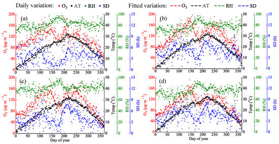
Figure A1.
Daily variation of O3 and meteorological conditions, including air temperature (AT), relative humility (RH), and sunshine duration (SD) over the four capital cities (a) Shanghai, (b) Nanjing, (c) Hangzhou, (d) Hefei in the Yangtze River Delta.
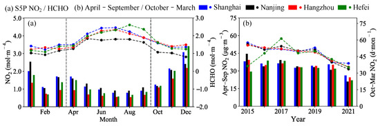
Figure A2.
(a) Satellite observed Daily HCHO and NO2 column densities, and (b) ground-level yearly NO2 variation from dense measurements over the over the four capital cities (blue: Shanghai, black: Nanjing, red: Hangzhou, green: Hefei) in the Yangtze River Delta.
References
- Feng, Z.; De Marco, A.; Anav, A.; Gualtieri, M.; Sicard, P.; Tian, H.; Fornasier, F.; Tao, F.; Guo, A.; Paoletti, E. Economic losses due to ozone impacts on human health, forest productivity and crop yield across China. Environ. Int. 2019, 131, 104966. [Google Scholar] [CrossRef] [PubMed]
- Sicard, P.; Augustaitis, A.; Belyazid, S.; Calfapietra, C.; Marco, A.D.; Fenn, M.; Bytnerowicz, A.; Grulke, N.; He, S.; Matyssek, R. Global topics and novel approaches in the study of air pollution, climate change and forest ecosystems. Environ. Pollut. 2016, 213, 977–987. [Google Scholar] [CrossRef] [PubMed]
- Stocker, T.; Qin, D.; Plattner, G.; Tignor, M.; Allen, S.; Boschung, J.; Nauels, A.; Xia, Y.; Bex, B.; Midgley, B. IPCC, 2013: Climate Change 2013: The Physical Science Basis—Contribution of Working Group I to the Fifth Assessment Report of the Intergovernmental Panel on Climate Change; Cambridge University Press: Cambridge, UK, 2013. [Google Scholar] [CrossRef]
- Juráň, S.; Grace, J.; Urban, O. Temporal Changes in Ozone Concentrations and Their Impact on Vegetation. Atmosphere 2021, 12, 82. [Google Scholar] [CrossRef]
- Xu, J.; Huang, X.; Wang, N.; Li, Y.; Ding, A. Understanding ozone pollution in the Yangtze River Delta of eastern China from the perspective of diurnal cycles. Sci. Total Environ. 2021, 752, 141928. [Google Scholar] [CrossRef]
- Lin, C.; Lau, A.K.H.; Fung, J.C.H.; Song, Y.; Li, Y.; Tao, M.; Lu, X.; Ma, J.; Lao, X.Q. Removing the effects of meteorological factors on changes in nitrogen dioxide and ozone concentrations in China from 2013 to 2020. Sci. Total Environ. 2021, 793, 148575. [Google Scholar] [CrossRef] [PubMed]
- Zhang, Y.; Yu, S.; Chen, X.; Li, Z.; Li, M.; Song, Z.; Liu, W.; Li, P.; Zhang, X.; Lichtfouse, E. Local production, downward and regional transport aggravated surface ozone pollution during the historical orange-alert large-scale ozone episode in eastern China. Environ. Chem. Lett. 2022, 20, 1577–1588. [Google Scholar] [CrossRef]
- Liu, P.; Song, H.; Wang, T.; Wang, F.; Li, X.; Miao, C.; Zhao, H. Effects of meteorological conditions and anthropogenic precursors on ground-level ozone concentrations in Chinese cities. Environ. Pollut. 2020, 262, 114366. [Google Scholar] [CrossRef]
- Li, K.; Chen, L.; Ying, F.; White, S.J.; Jang, C.; Wu, X.; Gao, X.; Hong, S.; Shen, J.; Azzi, M.; et al. Meteorological and chemical impacts on ozone formation: A case study in Hangzhou, China. Atmos. Res. 2017, 196, 40–52. [Google Scholar] [CrossRef]
- Lu, X.; Zhang, L.; Chen, Y.; Zhou, M.; Zheng, B.; Li, K.; Liu, Y.; Lin, J.; Fu, T.M.; Zhang, Q. Exploring 2016–2017 surface ozone pollution over China: Source contributions and meteorological influences. Atmos. Chem. Phys. 2019, 19, 8339–8361. [Google Scholar] [CrossRef] [Green Version]
- Thompson, M.L.; Reynolds, J.; Cox, L.H.; Guttorp, P.; Sampson, P.D. A review of statistical methods for the meteorological adjustment of tropospheric ozone. Atmos. Environ. 2001, 35, 617–630. [Google Scholar] [CrossRef]
- Dai, H.; Zhu, J.; Liao, H.; Li, J.; Liang, M.; Yang, Y.; Yue, X. Co-occurrence of ozone and PM2.5 pollution in the Yangtze River Delta over 2013–2019: Spatiotemporal distribution and meteorological conditions. Atmos. Res. 2021, 249, 105363. [Google Scholar] [CrossRef]
- Zhan, C.; Xie, M.; Liu, J.; Wang, T.; Xu, M.; Chen, B.; Li, S.; Zhuang, B.; Li, M. Surface Ozone in the Yangtze River Delta, China: A Synthesis of Basic Features, Meteorological Driving Factors, and Health Impacts. J. Geophys. Res. Atmos. 2021, 126, e2020JD033600. [Google Scholar] [CrossRef]
- Fan, M.-Y.; Zhang, Y.-L.; Lin, Y.-C.; Li, L.; Xie, F.; Hu, J.; Mozaffar, A.; Cao, F. Source apportionments of atmospheric volatile organic compounds in Nanjing, China during high ozone pollution season. Chemosphere 2021, 263, 128025. [Google Scholar] [CrossRef]
- Shu, L.; Wang, T.; Han, H.; Xie, M.; Chen, P.; Li, M.; Wu, H. Summertime ozone pollution in the Yangtze River Delta of eastern China during 2013–2017: Synoptic impacts and source apportionment. Environ. Pollut. 2020, 257, 113631. [Google Scholar] [CrossRef] [PubMed]
- Tang, K.; Zhang, H.; Feng, W.; Liao, H.; Hu, J.; Li, N. Increasing but Variable Trend of Surface Ozone in the Yangtze River Delta Region of China. Front. Environ. Sci. 2022, 10, 836191. [Google Scholar] [CrossRef]
- Kleinman, L.I. Low and high NOx tropospheric photochemistry. J. Geophys. Res. Atmos. 1994, 99, 16831–16838. [Google Scholar] [CrossRef]
- Li, Z.; Yu, S.; Li, M.; Chen, X.; Zhang, Y.; Song, Z.; Li, J.; Jiang, Y.; Liu, W.; Li, P.; et al. The Modeling Study about Impacts of Emission Control Policies for Chinese 14th Five-Year Plan on PM2.5 and O3 in Yangtze River Delta, China. Atmosphere 2021, 13, 26. [Google Scholar] [CrossRef]
- Liu, H.; Wang, X.M.; Pang, J.M.; He, K.B. Feasibility and difficulties of China’s new air quality standard compliance: PRD case of PM2.5 and ozone from 2010 to 2025. Atmos. Chem. Phys. 2013, 13, 12013–12027. [Google Scholar] [CrossRef]
- Kaser, L.; Peron, A.; Graus, M.; Striednig, M.; Wohlfahrt, G.; Juráň, S.; Karl, T. Interannual variability of terpenoid emissions in an alpine city. Atmos. Chem. Phys. 2022, 22, 5603–5618. [Google Scholar] [CrossRef]
- Wang, T.; Xue, L.; Feng, Z.; Dai, J.; Zhang, Y.; Tan, Y. Ground-level ozone pollution in China: A synthesis of recent findings on influencing factors and impacts. Environ. Res. Lett. 2022, 17, 63003. [Google Scholar] [CrossRef]
- Zhao, H.; Zheng, Y.; Zhang, Y.; Li, T. Evaluating the effects of surface O3 on three main food crops across China during 2015–2018. Environ. Pollut. 2020, 258, 113794. [Google Scholar] [CrossRef] [PubMed]
- Lu, X.; Hong, J.; Zhang, L.; Cooper, O.R.; Schultz, M.G.; Xu, X.; Wang, T.; Gao, M.; Zhao, Y.; Zhang, Y. Severe Surface Ozone Pollution in China: A Global Perspective. Environ. Sci. Technol. Lett. 2018, 5, 487–494. [Google Scholar] [CrossRef]
- Wang, T.; Xue, L.; Brimblecombe, P.; Lam, Y.F.; Li, L.; Zhang, L. Ozone pollution in China: A review of concentrations, meteorological influences, chemical precursors, and effects. Sci. Total Environ. 2017, 575, 1582–1596. [Google Scholar] [CrossRef] [PubMed]
- MEP. Ministry of Environmental Protection, 2012, Government of China. Ambient Air Quality Standards. GB 3095–2012. Available online: https://www.mee.gov.cn/ywgz/fgbz/bz/bzwb/dqhjbh/dqhjzlbz/201203/t20120302_224165.shtml (accessed on 20 July 2022). (In Chinese)
- Martin, R.V.; Fiore, A.M.; Van Donkelaar, A. Space-based diagnosis of surface ozone sensitivity to anthropogenic emissions. Geophys. Res. Lett. 2004, 31, L06120. [Google Scholar] [CrossRef]
- Eskes, H.; van Geffen, J.; Boersma, F.; Eichmann, K.-U.; Apituley, A.; Pedergnana, M.; Sneep, M.; Veefkind, J.; Loyola, D. Sentinel-5 Precursor/TROPOMI Level 2 Product User Manual Nitrogendioxide; Ministry of Infrastructure and Water Management: The Hague, The Netherlands, 2019. [Google Scholar]
- Gorelick, N.; Hancher, M.; Dixon, M.; Ilyushchenko, S.; Thau, D.; Moore, R. Google Earth Engine: Planetary-scale geospatial analysis for everyone. Remote Sens. Environ. 2017, 202, 18–27. [Google Scholar] [CrossRef]
- Jin, X.; Holloway, T. Spatial and temporal variability of ozone sensitivity over China observed from the Ozone Monitoring Instrument. J. Geophys. Res. Atmos. 2015, 120, 7229–7246. [Google Scholar] [CrossRef]
- Wang, Y.; Zhu, S.; Ma, J.; Shen, J.; Wang, P.; Wang, P.; Zhang, H. Enhanced atmospheric oxidation capacity and associated ozone increases during COVID-19 lockdown in the Yangtze River Delta. Sci. Total Environ. 2021, 768, 144796. [Google Scholar] [CrossRef]
- Young, P.J.; Archibald, A.T.; Bowman, K.W.; Lamarque, J.F.; Naik, V.; Stevenson, D.S.; Tilmes, S.; Voulgarakis, A.; Wild, O.; Bergmann, D.; et al. Pre-industrial to end 21st century projections of tropospheric ozone from the Atmospheric Chemistry and Climate Model Intercomparison Project (ACCMIP). Atmos. Chem. Phys. 2013, 13, 2063–2090. [Google Scholar] [CrossRef]
- Monks, P.S.; Archibald, A.T.; Colette, A.; Cooper, O.; Coyle, M.; Derwent, R.; Fowler, D.; Granier, C.; Law, K.S.; Mills, G.E.; et al. Tropospheric ozone and its precursors from the urban to the global scale from air quality to short-lived climate forcer. Atmos. Chem. Phys. 2015, 15, 8889–8973. [Google Scholar] [CrossRef] [Green Version]
- Zhan, C.; Xie, M.; Huang, C.; Liu, J.; Wang, T.; Xu, M.; Ma, C.; Yu, J.; Jiao, Y.; Li, M.; et al. Ozone affected by a succession of four landfall typhoons in the Yangtze River Delta, China: Major processes and health impacts. Atmos. Chem. Phys. 2020, 20, 13781–13799. [Google Scholar] [CrossRef]
- Shen, L.; Liu, J.; Zhao, T.; Xu, X.; Han, H.; Wang, H.; Shu, Z. Atmospheric transport drives regional interactions of ozone pollution in China. Sci. Total Environ. 2022, 830, 154634. [Google Scholar] [CrossRef] [PubMed]
- Yin, H.; Lu, X.; Sun, Y.; Li, K.; Gao, M.; Zheng, B.; Liu, C. Unprecedented decline in summertime surface ozone over eastern China in 2020 comparably attributable to anthropogenic emission reductions and meteorology. Environ. Res. Lett. 2021, 16, 124069. [Google Scholar] [CrossRef]
- Le, T.; Wang, Y.; Liu, L.; Yang, J.; Yung, Y.L.; Li, G.; Seinfeld, J.H. Unexpected air pollution with marked emission reductions during the COVID-19 outbreak in China. Science 2020, 369, 702–706. [Google Scholar] [CrossRef] [PubMed]
- Wang, N.; Xu, J.; Pei, C.; Tang, R.; Zhou, D.; Chen, Y.; Li, M.; Deng, X.; Deng, T.; Huang, X.; et al. Air Quality during COVID-19 Lockdown in the Yangtze River Delta and the Pearl River Delta: Two Different Responsive Mechanisms to Emission Reductions in China. Environ. Sci. Technol. 2021, 55, 5721–5730. [Google Scholar] [CrossRef] [PubMed]
- Ren, J.; Xie, S. Diagnosing ozone-NOx-VOC sensitivity and revealing causes of ozone increases in China based on 2013–2021 satellite retrievals. Atmos. Chem. Phys. Discuss. 2022. preprint. [Google Scholar] [CrossRef]
- Liu, S.; Liu, C.; Hu, Q.; Su, W.; Yang, X.; Lin, J.; Zhang, C.; Xing, C.; Ji, X.; Tan, W.; et al. Distinct Regimes of O3 Response to COVID-19 Lockdown in China. Atmosphere 2021, 12, 184. [Google Scholar] [CrossRef]
- Mao, Y.-H.; Yu, S.; Shang, Y.; Liao, H.; Li, N. Response of Summer Ozone to Precursor Emission Controls in the Yangtze River Delta Region. Front. Environ. Sci. 2022, 10, 864897. [Google Scholar] [CrossRef]
- Dong, Z.; Xing, J.; Zhang, F.; Wang, S.; Ding, D.; Wang, H.; Huang, C.; Zheng, H.; Jiang, Y.; Hao, J. Synergetic PM2.5 and O3 control strategy for the Yangtze River Delta, China. J. Environ. Sci. 2022, in press. [Google Scholar] [CrossRef]
- Wang, W.; van der A, R.; Ding, J.; van Weele, M.; Cheng, T. Spatial and temporal changes of the ozone sensitivity in China based on satellite and ground-based observations. Atmos. Chem. Phys. 2021, 21, 7253–7269. [Google Scholar] [CrossRef]
- Wang, M.; Chen, W.; Zhang, L.; Qin, W.; Zhang, Y.; Zhang, X.; Xie, X. Ozone pollution characteristics and sensitivity analysis using an observation-based model in Nanjing, Yangtze River Delta Region of China. J. Environ. Sci. 2020, 93, 13–22. [Google Scholar] [CrossRef]
- Wang, N.; Lyu, X.; Deng, X.; Huang, X.; Jiang, F.; Ding, A. Aggravating O3 pollution due to NOx emission control in eastern China. Sci. Total Environ. 2019, 677, 732–744. [Google Scholar] [CrossRef] [PubMed]
- Li, X.; Qin, M.; Li, L.; Gong, K.; Shen, H.; Li, J.; Hu, J. Examining the implications of photochemical indicators on the O3-NOx-VOC sensitivity and control strategies: A case study in the Yangtze River Delta (YRD), China. Atmos. Chem. Phys. Discuss. 2022, preprint. [Google Scholar] [CrossRef]
Publisher’s Note: MDPI stays neutral with regard to jurisdictional claims in published maps and institutional affiliations. |
© 2022 by the authors. Licensee MDPI, Basel, Switzerland. This article is an open access article distributed under the terms and conditions of the Creative Commons Attribution (CC BY) license (https://creativecommons.org/licenses/by/4.0/).