
Ground-Based Measurements of Cloud Properties at the Bucharest–Măgurele Cloudnet Station: First Results
 , ,
, , 
Abstract
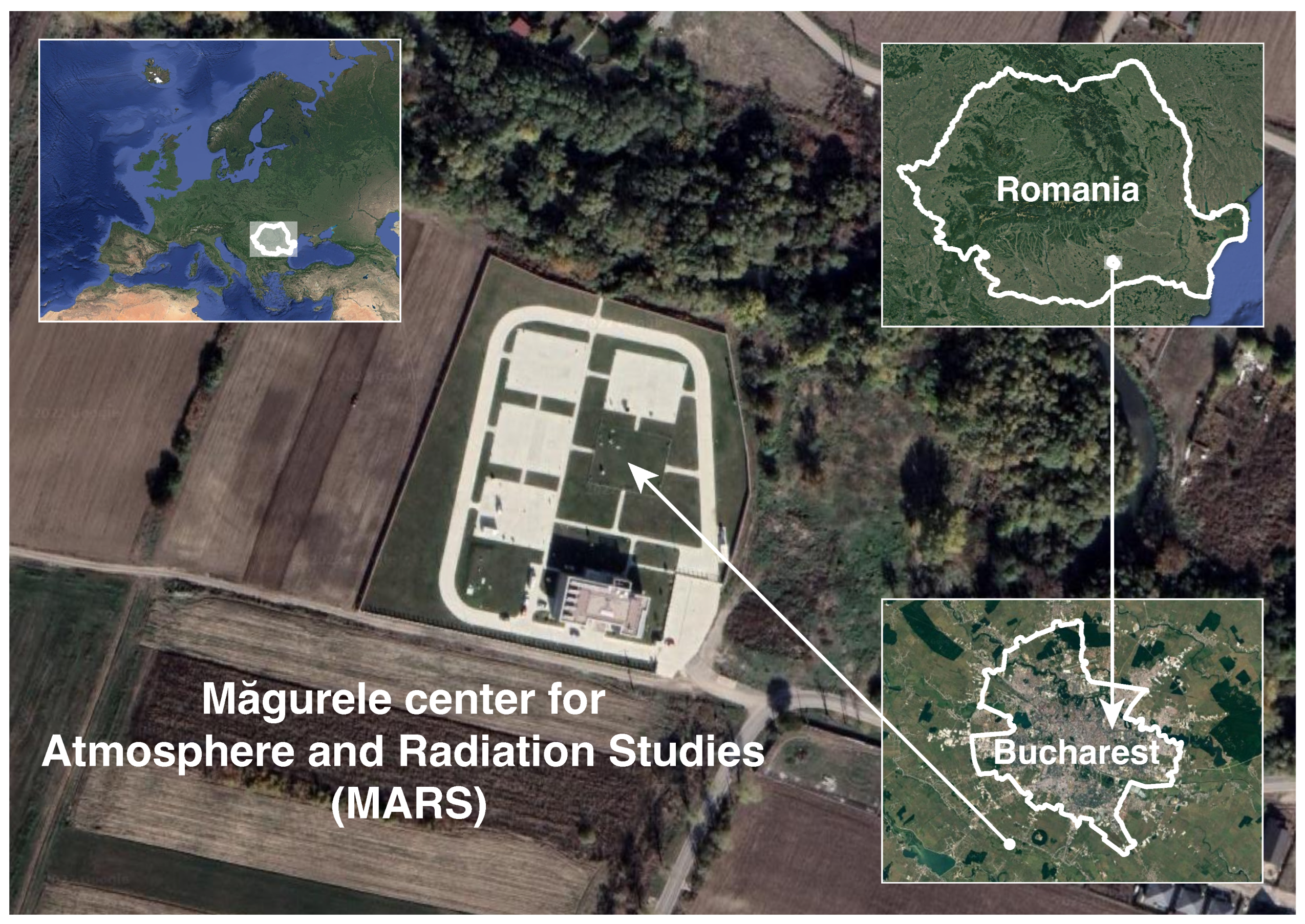
:1. Introduction
2. Data and Methods
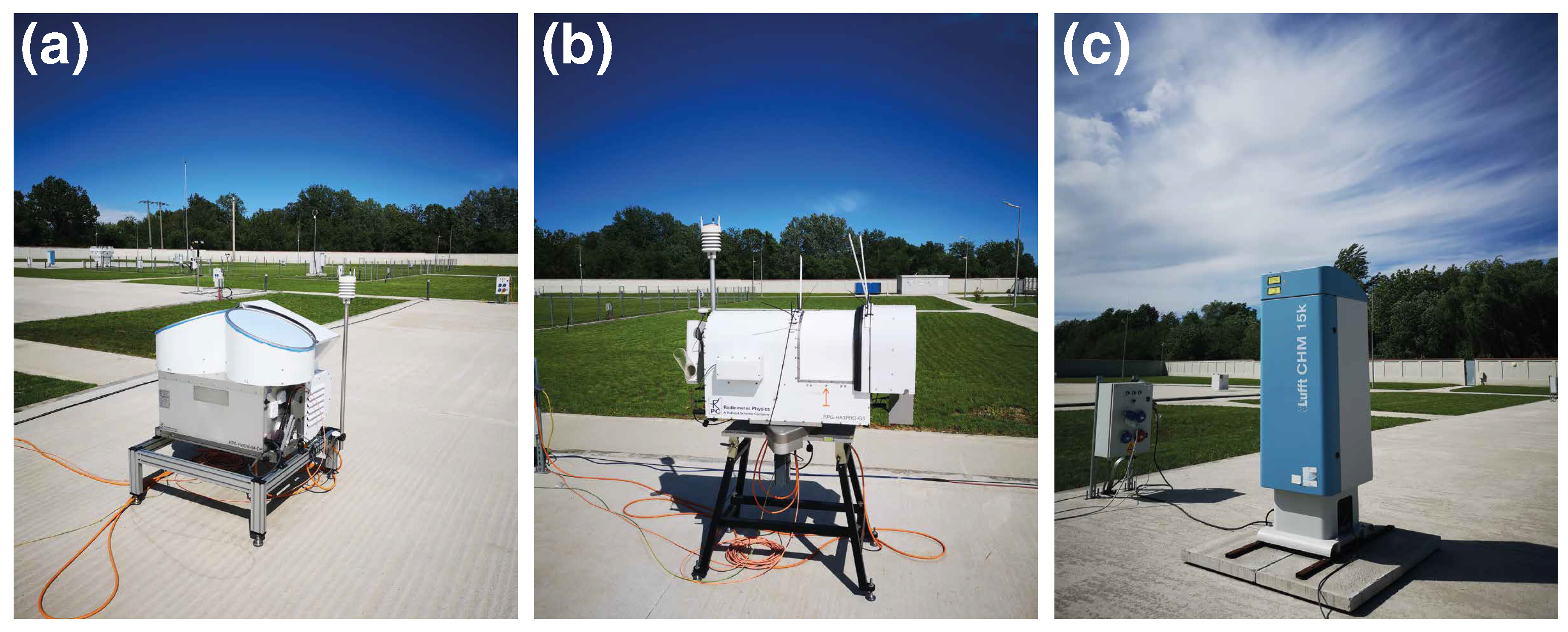
2.1. Cloud Radar
2.2. Microwave Radiometer
2.3. Ceilometer Data
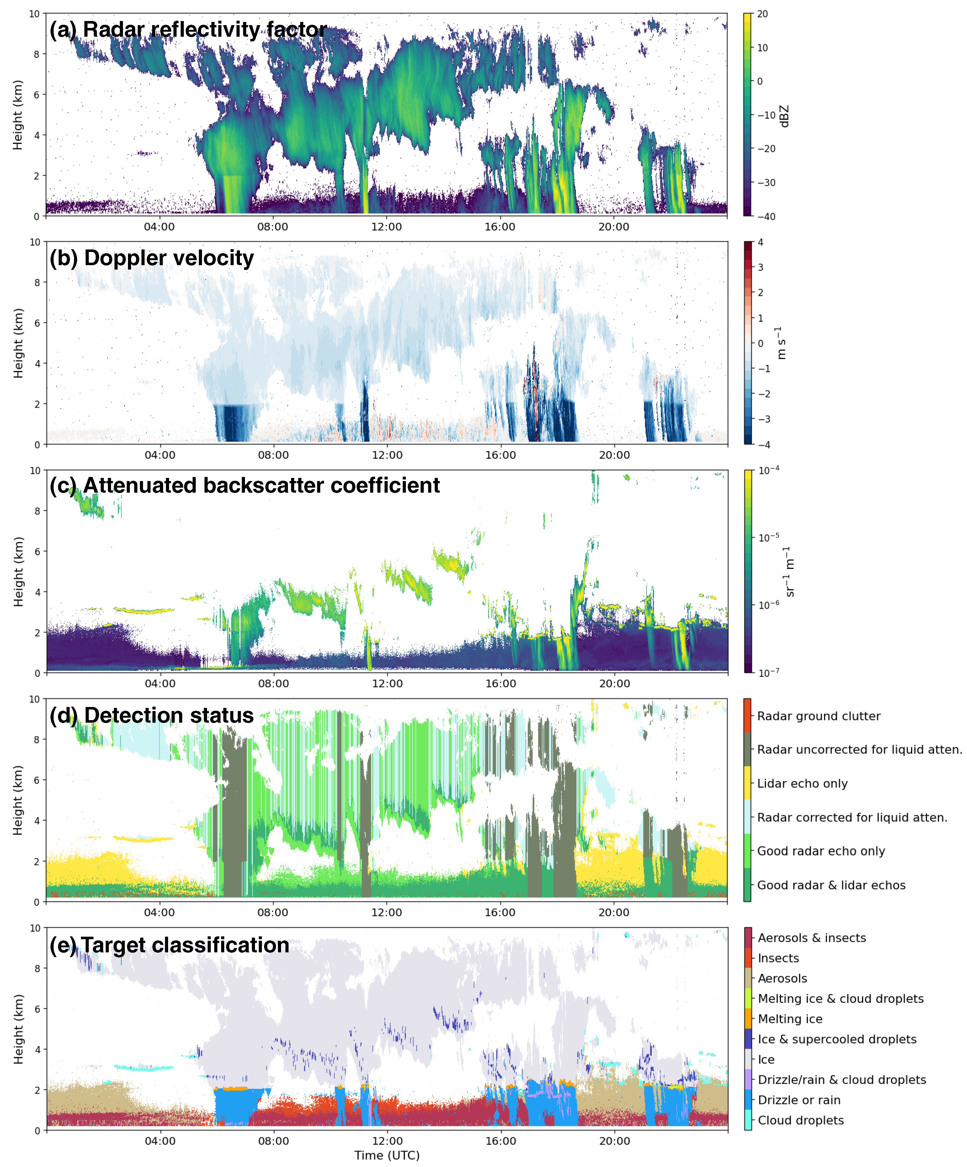
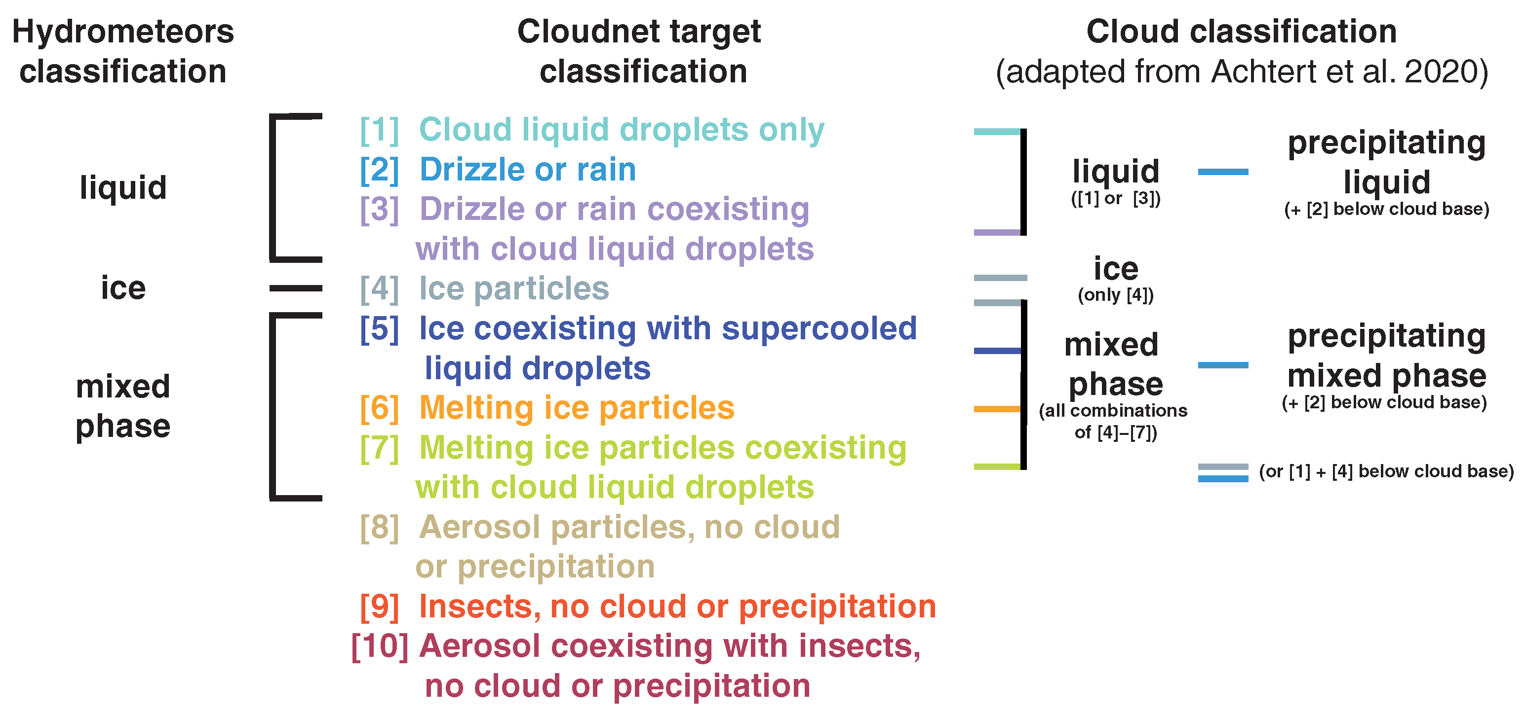
2.4. Hydrometeors and Cloud Classification
3. Results
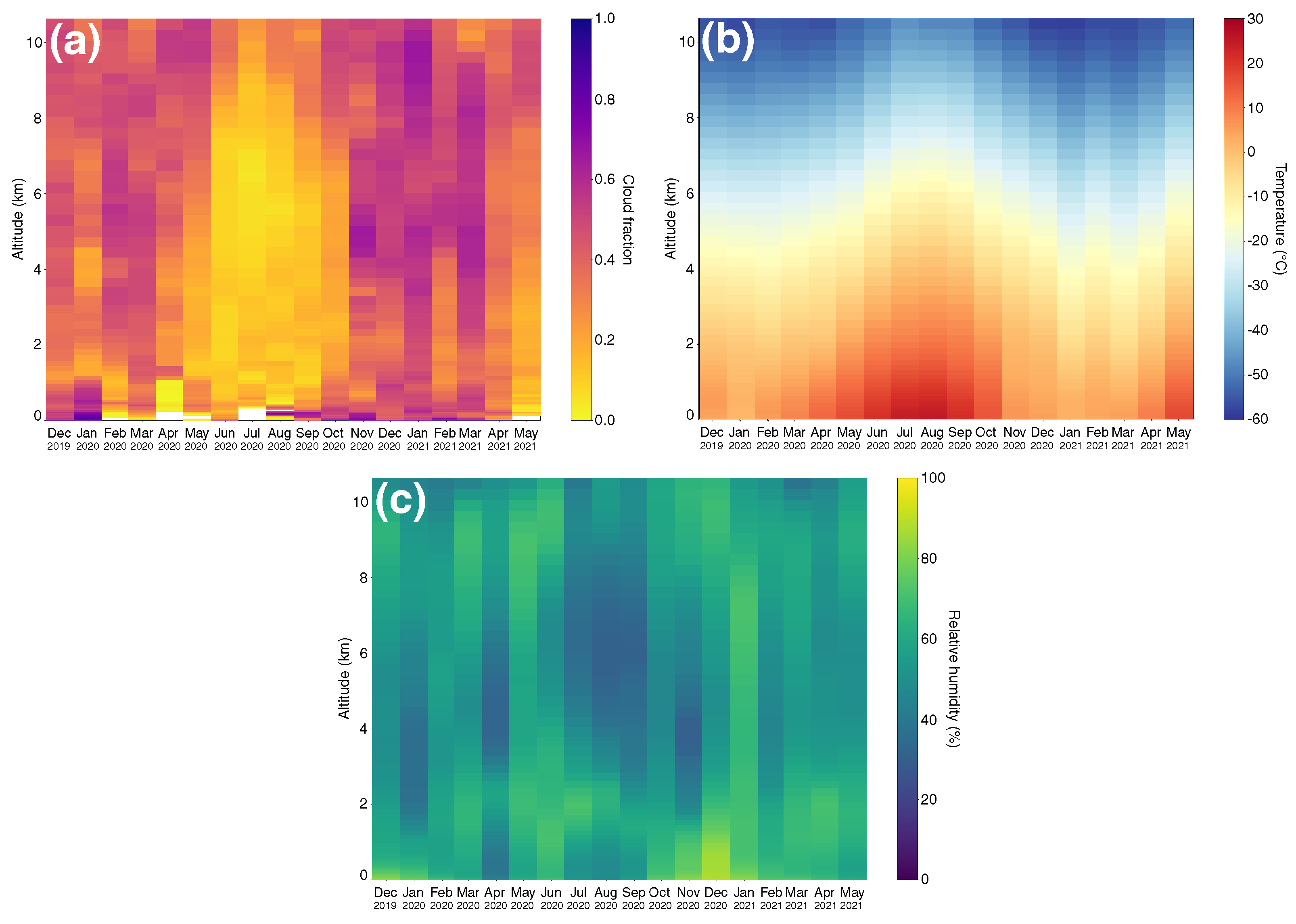
3.1. Environmental Characteristics
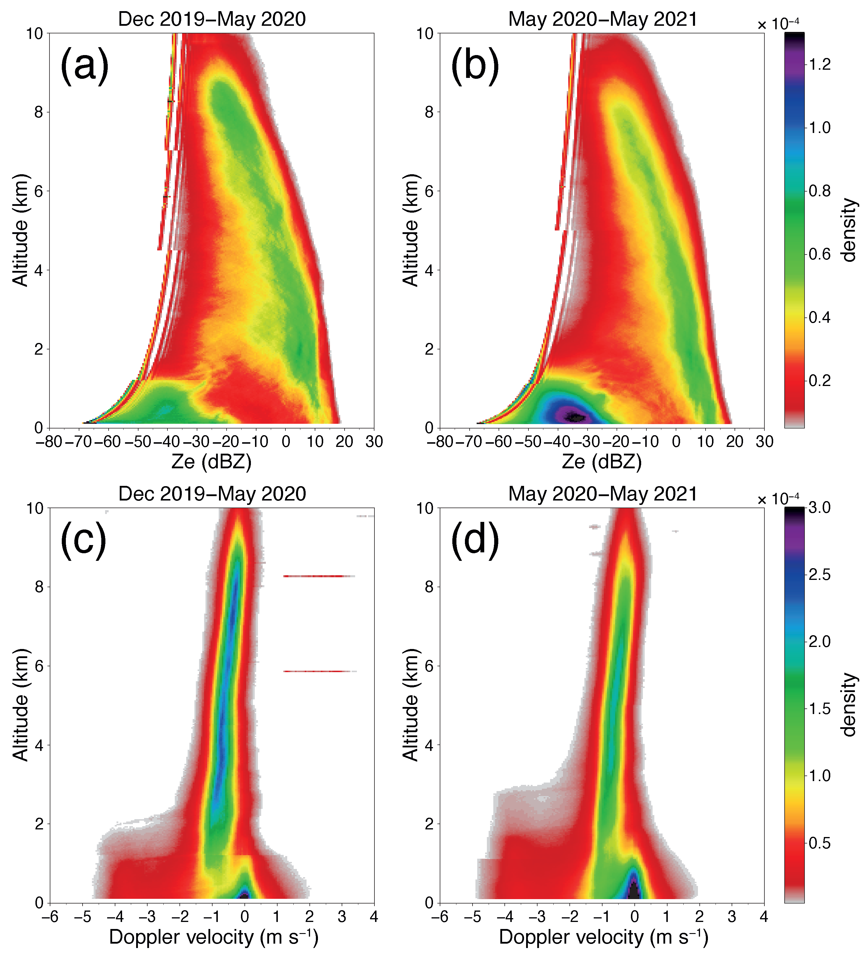
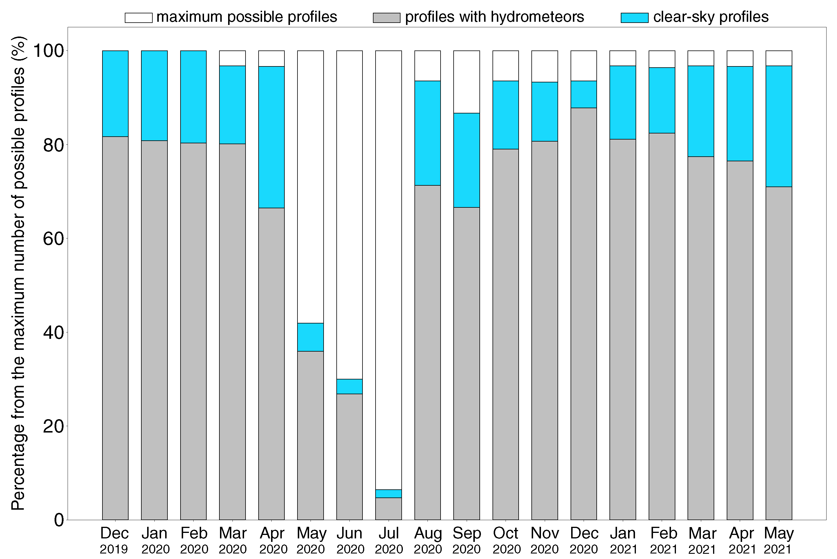
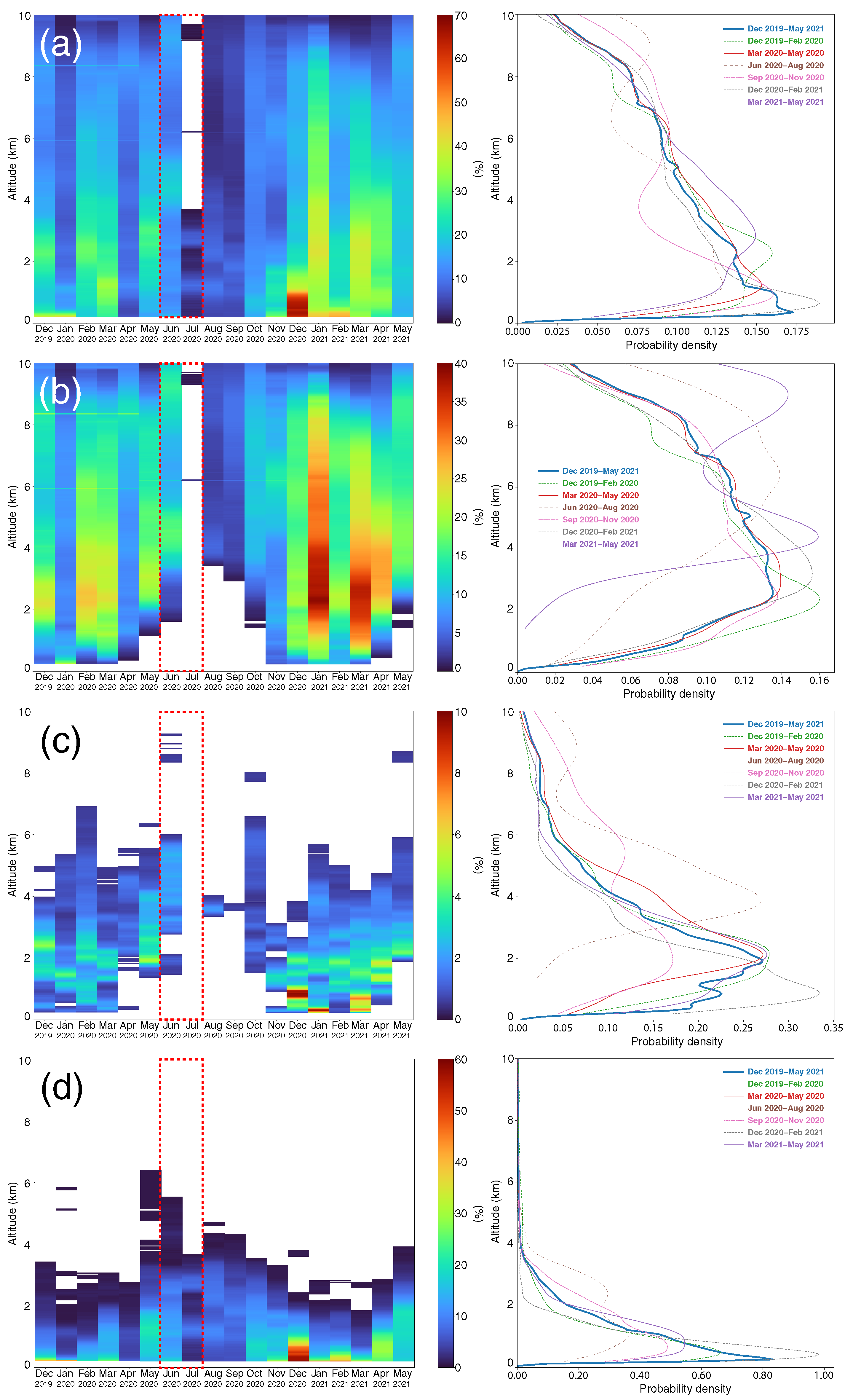
3.2. Hydrometeor Characteristics
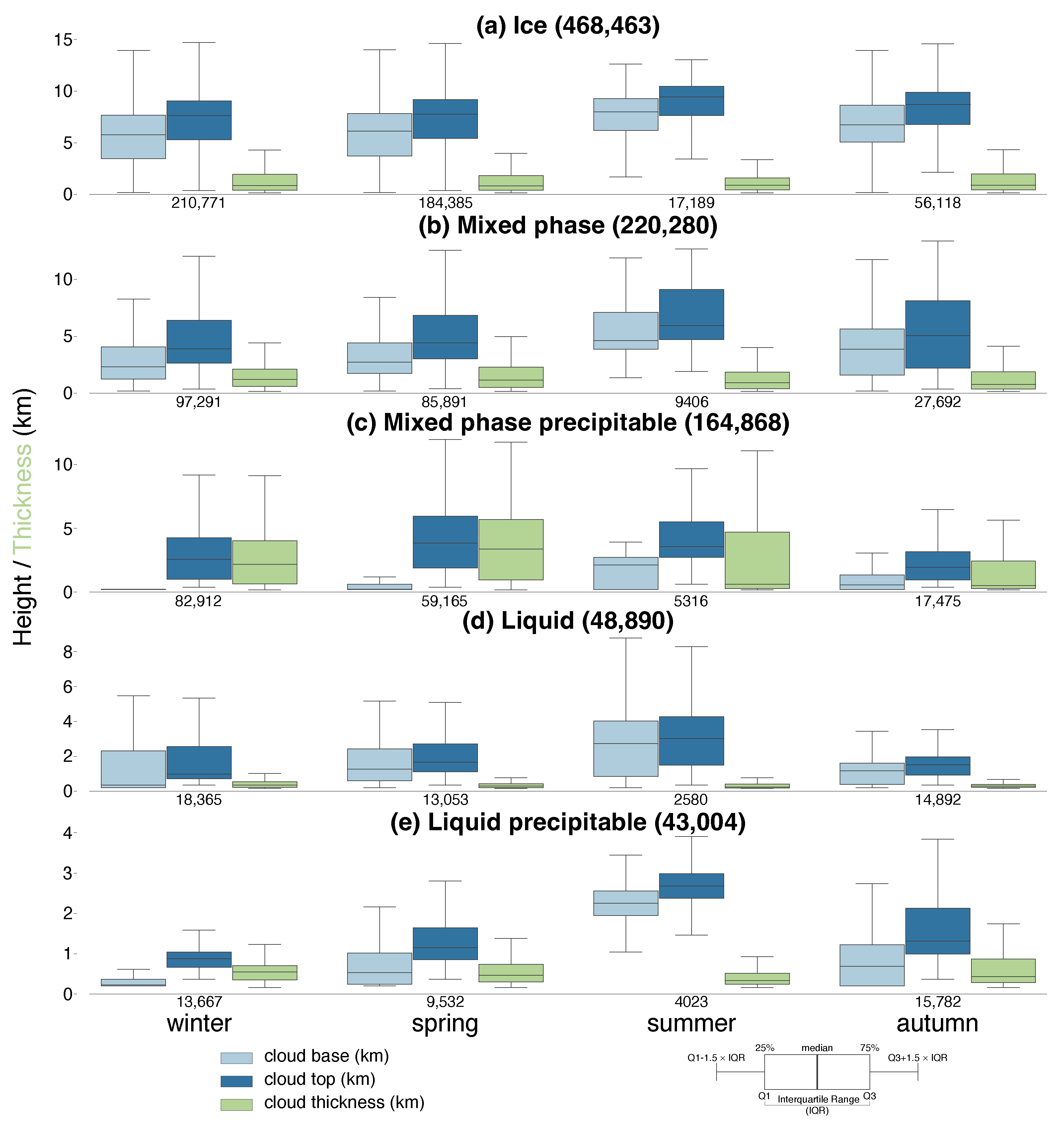
3.3. Cloud Characteristics
4. Conclusions
Author Contributions
Funding
Data Availability Statement
Acknowledgments
Conflicts of Interest
References
- Cesana, G.; Storelvmo, T. Improving climate projections by understanding how cloud phase affects radiation. J. Geophys. Res.-Atmos. 2017, 122, 4594–4599. [Google Scholar] [CrossRef]
- Matus, A.V.; L’Ecuyer, T.S. The role of cloud phase in Earth’s radiation budget. J. Geophys. Res.-Atmos. 2017, 122, 2559–2578. [Google Scholar] [CrossRef]
- McFarquhar, G.M.; Bretherton, C.S.; Marchand, R.; Protat, A.; DeMott, P.J.; Alexander, S.P.; Roberts, G.C.; Twohy, C.H.; Toohey, D.; Siems, S.; et al. Observations of Clouds, Aerosols, Precipitation, and Surface Radiation over the Southern Ocean: An Overview of CAPRICORN, MARCUS, MICRE, and SOCRATES. Bull. Am. Meteorol. Soc. 2021, 102, E894–E928. [Google Scholar] [CrossRef]
- Löhnert, U.; Schween, J.H.; Acquistapace, C.; Ebell, K.; Maahn, M.; Barrera-Verdejo, M.; Hirsikko, A.; Bohn, B.; Knaps, A.; O’Connor, E.; et al. JOYCE: Jülich Observatory for Cloud Evolution. Bull. Am. Meteorol. Soc. 2015, 96, 1157–1174. [Google Scholar] [CrossRef]
- Haeffelin, M.; Barthès, L.; Bock, O.; Boitel, C.; Bony, S.; Bouniol, D.; Chepfer, H.; Chiriaco, M.; Cuesta, J.; Delanoë, J.; et al. SIRTA, a ground-based atmospheric observatory for cloud and aerosol research. Ann. Geophys. 2005, 23, 253–275. [Google Scholar] [CrossRef]
- Stephens, G.; Winker, D.; Pelon, J.; Trepte, C.; Vane, D.; Yuhas, C.; L’Ecuyer, T.; Lebsock, M. CloudSat and CALIPSO within the A-Train: Ten Years of Actively Observing the Earth System. Bull. Am. Meteor. Soc. 2018, 99, 569–581. [Google Scholar] [CrossRef]
- Loeb, N.G.; Doelling, D.R.; Wang, H.; Su, W.; Nguyen, C.; Corbett, J.G.; Liang, L.; Mitrescu, C.; Rose, F.G.; Kato, S. Clouds and the Earth’s Radiant Energy System (CERES) Energy Balanced and Filled (EBAF) Top-of-Atmosphere (TOA) Edition-4.0 Data Product. J. Clim. 2018, 31, 895–918. [Google Scholar] [CrossRef]
- Mather, J.H.; Voyles, J.W. The ARM Climate Research Facility: A review of structure and capabilities. Bull. Am. Meteor. Soc. 2013, 94, 377–392. [Google Scholar] [CrossRef]
- Illingworth, A.J.; Hogan, R.J.; O’Connor, E.J.; Bouniol, D.; Brooks, M.E.; Delanoë, J.; Donovan, D.P.; Eastment, J.D.; Gaussiat, N.; Goddard, J.W.; et al. Cloudnet: Continuous evaluation of cloud profiles in seven operational models using ground-based observations. Bull. Am. Meteorol. Soc. 2007, 88, 883–898. [Google Scholar] [CrossRef]
- Tukiainen, S.; O’Connor, E.; Korpinen, A. CloudnetPy: A Python package for processing cloud remote sensing data. J. Open Source Softw. 2020, 5, 2123. [Google Scholar] [CrossRef]
- Hogan, R.J.; O’Connor, E.J. Facilitating Cloud Radar and Lidar Algorithms: The Cloudnet Instrument Synergy/Target Categorization Product; Cloudnet Documentation 14 pp; University of Reading: Reading, UK, 2004; Available online: http://www.cloud-net.org/data/products/categorize.html (accessed on 31 March 2022).
- O’Connor, E.J.; Hogan, R.J.; Illingworth, A.J. Retrieving Stratocumulus Drizzle Parameters Using Doppler Radar and Lidar. J. Appl. Meteorol. 2005, 44, 14–27. [Google Scholar] [CrossRef]
- Krasnov, O.A.; Russchenberg, H.W.J. A synergetic radar-lidar technique for the LWC retrieval in water clouds: Description and application to the Cloudnet data. In Proceedings of the 32d Conference on Radar Meteorology and 11th Conference on Mesoscale Processes, Albuquerque, NM, USA, 22–24 October 2005; p. 11. [Google Scholar]
- Hogan, R.J.; Mittermaier, M.P.; Illingworth, A.J. The retrieval of ice water content from radar reflectivity factor and temperature and its use in evaluating a mesoscale model. J. Appl. Meteor. Climatol. 2006, 45, 301–317. [Google Scholar] [CrossRef]
- van Zadelhoff, G.J.; Donovan, D.P.; Klein Baltink, H.; Boers, R. Comparing ice cloud microphysical properties using CloudNET and Atmospheric Radiation Measurement Program data. J. Geophys. Res. 2004, 109, D24214. [Google Scholar] [CrossRef]
- Bühl, J.; Seifert, P.; Myagkov, A.; Ansmann, A. Measuring ice- and liquid-water properties in mixed-phase cloud layers at the Leipzig Cloudnet station. Atmos. Chem. Phys. 2016, 16, 10609–10620. [Google Scholar] [CrossRef]
- Wandinger, U.; Seifert, P.; Engelmann, R.; Bühl, J.; Wagner, J.; Schmidt, J.; Pospichal, B.; Baars, H.; Schwarz, A.; Kanitz, T.; et al. Observation of aerosol–cloud–turbulence interaction with integrated remote-sensing instrumentation. In Proceedings of the 9th International Symposium on Tropospheric Profiling, L’Aquila, Italy, 3–7 September 2012. [Google Scholar]
- Achtert, P.; O’Connor, E.J.; Brooks, I.M.; Sotiropoulou, G.; Shupe, M.D.; Pospichal, B.; Brooks, B.J.; Tjernström, M. Properties of Arctic liquid and mixed-phase clouds from shipborne Cloudnet observations during ACSE 2014. Atmos. Chem. Phys. 2020, 20, 14983–15002. [Google Scholar] [CrossRef]
- Nomokonova, T.; Ebell, K.; Löhnert, U.; Maturilli, M.; Ritter, C.; O’Connor, E. Statistics on clouds and their relation to thermodynamic conditions at Ny-Ålesund using ground-based sensor synergy. Atmos. Chem. Phys. 2019, 19, 4105–4126. [Google Scholar] [CrossRef]
- Marinou, E.; Voudouri, K.; Tsikoudi, I.; Drakaki, E.; Tsekeri, A.; Rosoldi, M.; Ene, D.; Baars, H.; O’Connor, E.; Amiridis, V.; et al. Geometrical and microphysical properties of clouds formed in the presence of dust above the Eastern Mediterranean. Remote Sens. 2021, 13, 5001. [Google Scholar] [CrossRef]
- Ştefan, S.; Ungureanu, I.; Grigoraş, C. A survey of cloud cover over Măgurele, Romania using ceilometer and satellite data. Rom. Rep. Phys. 2014, 66, 812–822. [Google Scholar]
- Saftoiu Golea, G.L.; Stefan, S.; Antonescu, B.; Iorga, G.; Livio, B. Characteristics of Stratocumulus clouds over Bucharest—Magurele. Rom. Rep. Phys. 2022, 74, 705. [Google Scholar]
- Paraschivescu, M.; Râmbu, N.; Ştefan, S. Atmospheric circulations associated to the interannual variability of cumulonimbus cloud frequency in the southern part of Romania. Int. J. Climatol. 2012, 32, 920–928. [Google Scholar] [CrossRef]
- Beck, H.; Zimmermann, N.; McVicar, T.; Vergopolan, N.; Berg, A.; Wood, E. Present and future Köppen–Geiger climate classification maps at 1-km resolution. Sci. Data 2018, 5, 1802214. [Google Scholar] [CrossRef] [PubMed]
- Fragkos, K.; Antonescu, B.; Giles, D.M.; Ene, D.; Boldeanu, M.; Efstathiou, G.A.; Belegante, L.; Nicolae, D. Assessment of the total precipitable water from a sun photometer, microwave radiometer and radiosondes at a continental site in southeastern Europe. Atmos. Meas. Tech. 2019, 12, 1979–1997. [Google Scholar] [CrossRef] [Green Version]
- Adam, M.; Stachlewska, I.S.; Mona, L.; Papagiannopoulos, N.; Bravo-Aranda, J.A.; Sicard, M.; Nicolae, D.N.; Belegante, L.; Janicka, L.; Szczepanik, D.; et al. Biomass burning events measured by lidars in EARLINET—Part 2: Optical properties investigation. Atmos. Chem. Phys. Discuss. 2021, 2021, 1–36. [Google Scholar] [CrossRef]
- Nicolae, D.; Vasilescu, J.; Talianu, C.; Binietoglou, I.; Nicolae, V.; Andrei, S.; Antonescu, B. A neural network aerosol-typing algorithm based on lidar data. Atmos. Chem. Phys. 2018, 18, 14511–14537. [Google Scholar] [CrossRef]
- Mărmureanu, L.; Marin, C.A.; Andrei, S.; Antonescu, B.; Ene, D.; Boldeanu, M.; Vasilescu, J.; Viţelaru, C.; Cadar, O.; Levei, E. Orange Snow—A Saharan Dust Intrusion over Romania During Winter Conditions. Remote Sens. 2019, 11, 2466. [Google Scholar] [CrossRef]
- QGIS.org. QGIS Geographic Information System. QGIS Association. 2022. Available online: http://www.qgis.org (accessed on 5 July 2022).
- Küchler, N.; Kneifel, S.; Löhnert, U.; Kollias, P.; Czekala, H.; Rose, T. A W-Band Radar–Radiometer System for Accurate and Continuous Monitoring of Clouds and Precipitation. J. Atmos. Ocean. Technol. 2017, 34, 2375–2392. [Google Scholar] [CrossRef]
- Houze, R.A., Jr.; Wilton, D.C.; Smull, B.F. Monsoon convection in the Himalayan region as seen by the TRMM Precipitation Radar. Quart. J. Roy. Meteor. Soc. 2007, 133, 1389–1411. [Google Scholar] [CrossRef]
- Ansmann, A.; Fruntke, J.; Engelmann, R. Updraft and downdraft characterization with Doppler lidar: Cloud-free versus cumuli-topped mixed layer. Atmos. Chem. Phys. 2010, 10, 7845–7858. [Google Scholar] [CrossRef]
- Rose, T.; Crewell, S.; Löhnert, U.; Simmer, C. A network suitable microwave radiometer for operational monitoring of the cloudy atmosphere. Atmos. Res. 2005, 75, 183–200. [Google Scholar] [CrossRef]
- Löhnert, U.; Crewell, S. Accuracy of cloud liquid water path from ground-based microwave radiometry: Part I. Dependency on cloud model statistics and precipitation. Radio Sci. 2003, 38, 8041. [Google Scholar] [CrossRef]
- Cimini, D.; Hewison, T.J.; Martin, L.; Güldner, J.; Gaffard, C.; Marzano, F.S. Temperature and humidity profile retrievals from ground-based microwave radiometers during TUC. Meteor. Z. 2006, 15, 45–56. [Google Scholar] [CrossRef]
- Löhnert, U.; Turner, D.D.; Crewell, S. Ground-based temperature and humidity profiling using spectral infrared and microwave Observations. Part I: Simulated retrieval performance in clear-sky conditions. J. Appl. Meteor. Climatol. 2009, 48, 1017–1032. [Google Scholar] [CrossRef]
- Adam, M.; Fragkos, K.; Binietoglou, I.; Wang, D.; Stachlewska, I.S.; Belegante, L.; Nicolae, V. Towards Early Detection of Tropospheric Aerosol Layers Using Monitoring with Ceilometer, Photometer, and Air Mass Trajectories. Remote Sens. 2022, 14, 1217. [Google Scholar] [CrossRef]
- O’Connor, E.J.; Illingworth, A.J.; Hogan, R.J. A technique for autocalibration of cloud lidar. J. Atmos. Ocean. Technol. 2004, 21, 777–786. [Google Scholar] [CrossRef]
- CLU. Cloud Profiling Product: Classification; 2019-12-01 to 2021-05-31; from Bucharest Romania. Generated by the Cloud Profiling Unit of the ACTRIS Data Centre. 2022. Available online: https://hdl.handle.net/21.12132/2.a83ab8e12c794345 (accessed on 1 December 2021).
- CLU. ECMWF Model Data; 2019-12-01 to 2020-05-31; from Bucharest, Romania. Generated by the Cloud Profiling Unit of the ACTRIS Data Centre. 2022. Available online: https://hdl.handle.net/21.12132/2.7bb01f12416849ea (accessed on 1 December 2021).
- Wypych, A.; Bochenek, B.; Różycki, M. Atmospheric Moisture Content over Europe and the Northern Atlantic. Atmosphere 2018, 9, 18. [Google Scholar] [CrossRef] [Green Version]


| Instrument | Measured Parameters | Temporal Resolution | Spatial Resolution | Retrieved Parameters |
|---|---|---|---|---|
| RPG 94 GHz | Doppler spectrum | 4.96 s | 29.8–42.1 m | cloud presence |
| cloud radar | reflectivity | 2.97 s | 27.1–51.1 m | and boundaries |
| LWP at 89 GHz | (see Table 2) | (see Table 2) | ||
| HATPRO G5 | brightness temperatures | 60 s | column integrated | liquid water path |
| microwave radiometer | measurements | |||
| CHM 15K | profiles of attenuated | 30 s | 15 m | cloud base |
| ceilometer | backscatter coefficient | height |
| Attributes | 1 | 2 | 3 | 4 |
|---|---|---|---|---|
| Chirp sequence 1 used between December 2019 and May 2020 | ||||
| Integration Time (s) | 0.621 | 0.798 | 1.539 | 2.007 |
| Range Interval (m) | 100–1200 | 1200–4500 | 4500–6963 | 7000–13,152 |
| Range Resolution (m) | 29.8 | 29.8 | 29.8 | 42.1 |
| Nyquist Velocity (±m s) | 10.5 | 8.2 | 5.8 | 4.5 |
| Doppler FFT | 1024 | 512 | 512 | 512 |
| Total samples: 56,848,384 | Total FFTs: 79,872 Total duration: 4.96 s | |||
| Chirp sequence 2 used between May 2020 and May 2021 | ||||
| Integration Time (s) | 0.458 | 0.743 | 0.964 | 0.781 |
| Range Interval (m) | 100–1100 | 1100–5000 | 5000–10,000 | 10,000–15,000 |
| Range Resolution (m) | 27.1 | 30.4 | 31.1 | 51.1 |
| Nyquist Velocity (±m s) | 8.4 | 6.6 | 5.1 | 4.2 |
| Doppler FFT | 1024 | 512 | 512 | 512 |
| Total samples: 34,033,664 | Total FFTs: 47,104 Total duration: 2.97 s | |||
Publisher’s Note: MDPI stays neutral with regard to jurisdictional claims in published maps and institutional affiliations. |
© 2022 by the authors. Licensee MDPI, Basel, Switzerland. This article is an open access article distributed under the terms and conditions of the Creative Commons Attribution (CC BY) license (https://creativecommons.org/licenses/by/4.0/).
Share and Cite
Pîrloagă, R.; Ene, D.; Boldeanu, M.; Antonescu, B.; O’Connor, E.J.; Ştefan, S. Ground-Based Measurements of Cloud Properties at the Bucharest–Măgurele Cloudnet Station: First Results. Atmosphere 2022, 13, 1445. https://doi.org/10.3390/atmos13091445
Pîrloagă R, Ene D, Boldeanu M, Antonescu B, O’Connor EJ, Ştefan S. Ground-Based Measurements of Cloud Properties at the Bucharest–Măgurele Cloudnet Station: First Results. Atmosphere. 2022; 13(9):1445. https://doi.org/10.3390/atmos13091445
Chicago/Turabian StylePîrloagă, Răzvan, Dragoş Ene, Mihai Boldeanu, Bogdan Antonescu, Ewan J. O’Connor, and Sabina Ştefan. 2022. "Ground-Based Measurements of Cloud Properties at the Bucharest–Măgurele Cloudnet Station: First Results" Atmosphere 13, no. 9: 1445. https://doi.org/10.3390/atmos13091445
APA StylePîrloagă, R., Ene, D., Boldeanu, M., Antonescu, B., O’Connor, E. J., & Ştefan, S. (2022). Ground-Based Measurements of Cloud Properties at the Bucharest–Măgurele Cloudnet Station: First Results. Atmosphere, 13(9), 1445. https://doi.org/10.3390/atmos13091445