Simultaneous Monitoring of Outdoor PAHs and Particles in a French Peri-Urban Site during COVID Restrictions and the Winter Saharan Dust Event

Abstract

The presence of polycyclic aromatic hydrocarbons (PAHs) and particulate matter (PM) in air is known to provoke deleterious effects on human health. This work focused on the monitoring of PM and PAHs in the air over four weeks in a peri-urban site in Strasbourg (France), using a three-stage cascade impactor and a particle analyser allowing PM₁, PM_2.5 and PM₁₀ discrimination. Meteorological conditions were monitored to study their influence on the pollutant levels. The average PM₁₀ concentration of the cascade impactor and particle analyser varied from 11.8 to 80.2 µg/m³ and 10.6 to 220.2 µg/m³, respectively. The PAH total concentration ranged in 1.1–7.6 ng/m³ and a predominance of 5- and 6-ring PAHs was observed. PAHs were also more abundant in finer particles (PM₁). Specifically, identified PAHs are traffic tracers suggesting that vehicular emission was one of its main sources. Two pollution episodes, associated with either a Saharan dust wind episode or traffic pollution, were observed, and led to PM₁₀ and PM_2.5 surpassing the daily limit values established by the European Union despite the traffic limitations according to the COVID restrictions. The total PAH concentrations were the highest during these periods suggesting PAHs might be bound to and transported via dust particles.

1. Introduction

Air quality is a topic that has gained more and more interest in the last decades, as pollutants present in air are responsible for causing deleterious effects on human health, as well as impacting the environment [1]. An increasing effort has been made to monitor the different pollutants, and multiple policies and initiatives exist with the aim of limiting and controlling air pollution, including the Air Quality Guidelines established by the World Health Organization [2]. The European Union also has multiple directives regarding air quality, such as the 2008/50/EC Directive on Ambient Air Quality and Cleaner Air for Europe [3] and 2004/107/EC Directive relating to arsenic, cadmium, mercury, nickel and polycyclic aromatic hydrocarbons (PAHs) in ambient air [4].

There is a very large number of outdoor air pollutants, but some are most commonly monitored, such as nitric oxides (NO and NO₂), ozone (O₃) and carbon monoxide (CO), as well as particulate matter (PM) [1,5]. In urban environments, these air pollutants are mostly caused by vehicular emissions, with other anthropogenic contributions including power and petrochemical plants, and incinerators [1]. Natural pollution episodes, such as volcanic eruptions, sea sprays or dust events, can also contribute largely to a decrease of air quality at certain times [6].

Particulate matter (PM) is a pollutant of particular interest because it poses more risks to human health than other common air pollutants [7]. Airborne PMs consist of a complex mixture of solid and liquid particles suspended in the atmosphere that vary in size and chemical composition depending on how, when, and where they were formed [7,8]. PMs are typically classified according to their aerodynamic diameter (D_ae) in different fractions, as their effects to human health are dependent on their size. In general, smaller particles will enter more easily and more deeply in the respiratory tract, with particles < 1 µm being able to penetrate the alveoli [7]. It is also known that particles with D_ae < 10 µm have the most deleterious effects to human health. Furthermore, other species can be associated with PMs, such as nitrates, sulfates, and semi volatile organic compounds (SVOCs), contributing to the importance of monitoring and limiting the exposure to PMs. Considering how far particles can travel in the respiratory tract and the consequent health effects, three PM fractions are typically considered: PM₁₀ (D_ae < 10 µm), PM_2.5 (D_ae < 2.5 µm) and PM₁ (D_ae < 1 µm). In the Directive 2008/50/EC, the European Union established daily and annual mean levels of 50 µg/m³ and 40 µg/m³, respectively, for PM₁₀ and an annual average of 25 µg/m³ for PM_2.5 [3]. Similarly, the US Environmental Protection Agency (US EPA) established the National Ambient Air Quality Standards (NAAQS) for common pollutants in outdoor air [9]. In NAAQS, the guideline for PM₁₀ is a maximum annual average of 150 µg/m³, while for PM_2.5 they provided two threshold values: a 24-h average of 15 µg/m³ and an annual average of 35 µg/m³ [9].

PAHs are a class of organic compounds that has attracted a lot of attention in the past decades because of their negative effects to human health, namely their carcinogenicity, toxicity and mutagenicity [10]. PAHs are compounds that have multiple aromatic rings in their chemical structure, and they can be categorized according to their molecular weight or ring number into low molecular weight PAHs (LMW-PAHs), medium molecular weight PAHs (MMW-PAHs) and high molecular weight PAHs (HMW-PAHs).

PAHs are produced both naturally and anthropogenically [11,12]. Natural sources include volcanic eruptions, forest fires and organic matter decay [11,12], while anthropogenic sources, which account for most PAH occurrences, are mainly related to incomplete combustion of organic matter, such as fossil fuels, in different human activities, ranging from residential heating and cooking to industries and vehicle emissions [11,12]. These environmentally persistent pollutants are mostly introduced in the environment by their release into the atmosphere, where they can be found in two different fractions: gas phase and bound to particulate matter. PAH atmospheric concentrations depend on the emission source, which is related to the location (urban or rural site), and to the weather parameters such as wind speed [13,14], whereas their partitioning between gas and particle phases is influenced by the temperature [13]. The European Union also established a limit for these pollutants at a mean annual target of 1 ng/m³ for benzo(a)pyrene (BaP) because BaP is considered to be the marker for the carcinogenic risk of PAHs in ambient air [4].

In this work, the aim was to study the outdoor air quality in Strasbourg in terms of PM and PAHs bound to PM, during a 4-week period that included specific pollution episodes marked by a significant increase of pollutants such as a Saharan dust wind episode. Additionally, the campaign occurred when the COVID pandemic measures were in place, which included a curfew. The PM were quantified continuously with a particle analyser, but also collected during multiple days using a three-stage cascade impactor (gravimetric method) to compare the two methods. PAHs on the collected particles were also quantified with the objective to identify any correlations between PAHs and PM in the specific context of COVID restrictions with low traffic suggesting a possible smaller impact of tailpipe exhausts. The sampling during this period makes it possible to study the influence of Saharan dust particles on the air quality in Strasbourg. Pollution related to Saharan dust wind episodes is generally characterized in terms of PMs and their main composition [6,15]. It is worth noting that, to the best of our knowledge, no publication in the literature that quantified PAHs and considered meteorological conditions influence to their concentrations on the PMs of Saharan dust were found.

2. Materials and Methods

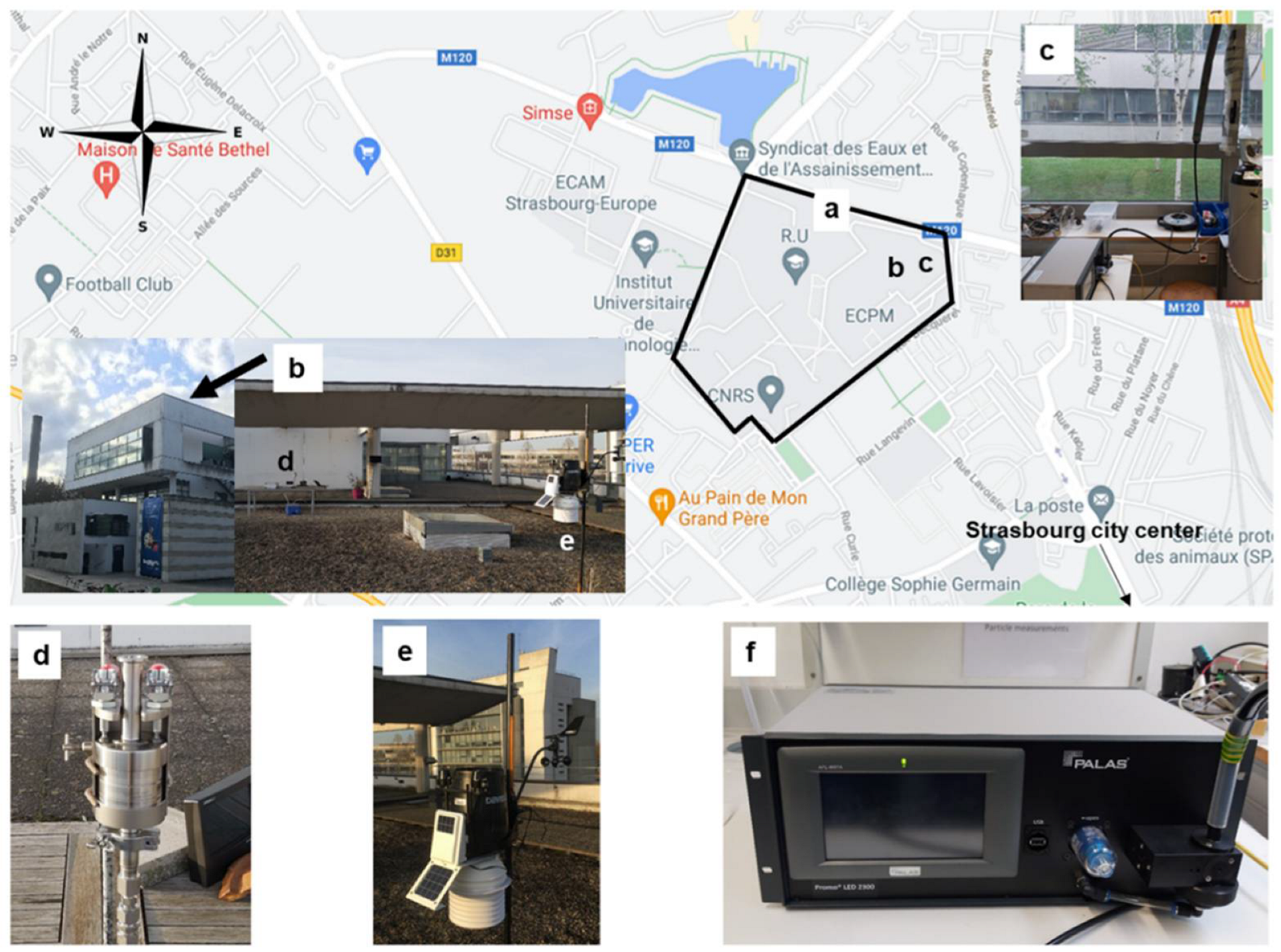
2.1. Experimental Campaign Locations

The campaign took place between 16 February and 15 March of 2021 on the Cronenbourg campus of the University of Strasbourg in Strasbourg, France during winter period. A curfew policy related to the COVID pandemic was also enforced during the campaign, restricting non-essential activities outside from 6 p.m. to 6 a.m. The campus is located near habitational neighborhoods, high-service bus stops, railways, and two highways (one in the east and one in southwest). The Strasbourg city center is approximately 5 km to the southeast side of the campus.

Two sampling sites, very close to each other, were used, as shown in Figure 1. The first sampling site, where the particles for PAH quantification were sampled by the three -stage cascade impactor (Figure 1b,d), was located on the rooftop of the École Européenne de Chimie, Polymères et Matériaux (ECPM) (48°36′27.4″ N 7°42′56.7″ E), above the 3rd floor. This location was chosen for its position on the Cronenbourg campus and for its proximity to a main road (Route de Hausbergen), as well as for the easy access for equipment installation and maintenance. In this site, a weather station (Vantage Pro 2 ISS, Davis Instrument) was installed to monitor multiple weather parameters during the campaign (temperature, relative humidity, wind speed and solar radiation). The weather data was stored with a time interval of 5 min.

The second sampling site using the particle analyser (Figure 1c,f) was outside, adjacent to our laboratory in the building R4 of the Institut de Chimie et Procédés pour l’Énergie, l’Environment et la Santé (ICPEES) (48°36′28.5″ N 7°43′02.2″ E). In this sampling site, the airborne particle concentration was continuously monitored and the necessity to maintain the particle analyser indoors, preferably in the laboratory, was the reason for its selection. As seen in Figure 1, the particle analyser was placed in the laboratory and the air sampling was performed by an antistatic tube, connected to particle analyser inlet, passing through the laboratory window that was posteriorly isolated.

The sampling campaign was divided in 8 sampling periods, also distinguishing between working days (WD) and weekend periods (WE). Thus, the monitoring campaign comprised 4 WD periods and 4 WE periods. A detailed summary of the experimental campaign calendar [16,17,18] can be found in Figure S1 of the Supplementary Materials.

2.2. Particulate Matter Sampling Methodology

As mentioned in Section 2.1, two different particle samplings were performed: a three-stage cascade impactor (gravimetric method) was used in the first sampling site, and a particle analyser (optical measurement) in the second nearby sampling site. Note that the measurements could not be replicated due to the availability of one cascade impactor and one analyser.

2.2.1. Three-Stage Cascade Impactor

The first sampling was performed with a commercial manual three-stages size fractionating cascade impactor (DEKATI, Impactor PM-10/PM-2.5/PM-1) connected to a vacuum pump (Thomas VTE3, Gardner Denver). The work principles of a cascade impactor have been described elsewhere [19], but briefly, the impactor operates based on inertial classification and gravimetric analysis of the particles present in air. Particulate matter is, thus, collected on the three stages of the impactor depending on their aerodynamic diameter (D_ae) in the following particle size ranges: D_ae > 10 µm, 10 µm > D_ae > 2.5 µm, and 2.5 µm > D_ae > 1 µm (Figure S2). The presence of a backup filter allows the collection of particles with D_ae < 1 µm.

To collect the particulate matter, glass microfiber filters (GFF) (Dominique Dutscher, 47 mm, pore size: 0.7 µm) were installed in the three stages and as backup filter and the filters’ sizes were adapted to the calibrated collection plates (25 mm for the three-stage collection plates and 47 mm for the backup filter). The air flow rate for the impactor was fixed at 1.8 m³/h (30 L/min). In order to evaluate the differences in air quality during working days (WD) and the weekend (WE), the filters of the impactor were collected and changed on Monday morning and on Friday afternoon, during the four weeks of the sampling campaign. Information on the duration of each period, as well as the volume of air sampled, can be found in

Table 1. Sampling periods and details of the 3-cascade impactor.

Period	Start		End		Duration (h)	Flow (m3/h)	Air Volume (m3)
	Date	Hour	Date	Hour
WD1	16 February 2021	15:49	19 February 2021	16:05	72.27	1.8	130.08
WE1	19 February 2021	16:42	22 February 2021	8:57	64.25	1.8	115.65
WD2	22 February 2021	9:45	26 February 2021	15:36	101.85	1.8	183.33
WE2	26 February 2021	16:10	1 March 2021	8:58	64.80	1.8	116.64
WD3	1 March 2021	9:37	5 March 2021	15:38	102.02	1.8	183.63
WE3	5 March 2021	16:06	8 March 2021	9:03	64.95	1.8	116.91
WD4	8 March 2021	9:29	12 March 2021	15:36	102.12	1.8	183.81
WE4	12 March 2021	16:12	15 March 2021	9:12	65.00	1.8	117.00

.

Before the sampling campaign, the filters were prepared by washing with acetonitrile (ACN) two times in an ultrasonic bath (Sonorex, Bandelin), for a minimum of 10 min, followed by drying at 50 °C for at least one hour, to ensure the elimination of possible contaminants. Blank filters were also prepared following the same methodology as the filters used for sampling but without installing them on the cascade impactor. After sampling, the filters were stored in Petri dishes covered with aluminum foil to protect them from light and stored in a refrigerator until further sample preparation and analysis.

For the quantification of particles in air, the filters were initially weighed three times before sampling, to measure the initial filter masses, using a balance (Kern ADB 200-4, accuracy of 0.1 mg). After sampling, the filters were weighed again three times and the mass of collected PM (in µg) was determined by subtracting the average of the final mass of the filter after sampling with the average of the initial mass of the filter, corrected by the blank filters. To obtain the particulate matter concentration, these values were divided by the total volume of sampled air (in m³).

2.2.2. Particle Analyser

A PM analyser (Palas Promo LED 2300) was used for a continuous real-time analysis of particles in air. Palas Promo LED 2300 measures particles based on optical light scattering, in a size range between 0.145 and 100 µm and up to 20,000 particles/cm³ in terms of concentration, according to the manufacturer.

The sampling flow rate was 4.8 L/min according to the manufacturer specifications. The data acquired by the equipment was stored every minute and PM values as particle concentration in number (particles/cm³) and in mass (µg/m³) were exported using the software PDAnalyze. The PM values were calculated by the software through a complex Palas environmental algorithm that considers different densities and refractive indexes for the particulate matter.

2.3. Extraction and Chemical Analysis of Extracted Organic Phases

The filters after sampling went through an extraction step using an accelerated solvent extractor (ASE 300, Dionex). In summary, the filters were placed in 34-mL cells, along with glass beads to reduce the solvent volume, and ACN as the solvent for extraction. The extraction was done at 150 °C and 1500 psi (103.4 bar), with 7-min cell heating, two 10-min static states, and 5 min of purging. Approximately 70 mL of ACN were used in each extraction and this extract volume was reduced to approximately 1 mL by evaporation under ambient conditions. The extracts were filtered through 0.20 µm syringe filters and/or centrifugated for 5 min at 1600× g in a centrifuge to eliminate eventual remaining particles. The extract final volume after evaporation was determined by weighing.

The extracts were then analysed by a High-Performance Liquid Chromatography (HPLC) system (Thermo Electron Corporation, Spectra System) equipped with a C₁₈ Pinnacle II PAH column (Restek, 150 mm × 3.2 mm ID, 4.0 µm particle size) and a C₁₈ Pinnacle II PAH guard column (Restek, 10 mm × 4.0 mm ID, 4.0 µm particle size). The HPLC system was coupled with a Diode Array Detector (DAD) (Thermo Finnigan, Spectra System UV6000LP) and a Fluorescence Detector (Thermo Scientific, Finnigan Surveyor FL Plus). HPLC was chosen because it is a commonly used analytical method in the quantification of PAHs in environmental samples [19]. A method using the same columns had been established in a previous work [19] and it was followed in this work with only slight modifications.

Oven temperature was set to 30 °C and the mobile phase was ACN and water (flow rate of 1 mL/min). The elution gradient was adapted from previous work [19] and it started with 50:50 (ACN:H₂O); after 8 min, it was changed to 60:40 (ACN:H₂O); then 70:30 (ACN:H₂O) after 10 min; 100:0 (ACN:H₂O) was the gradient between 21 and 25 min, and finally, at 25.1 min, the gradient was changed back to 50:50 (ACN:H₂O) and maintained until 30 min, which was the overall run time.

As mentioned before, the EU only has a target value for BaP; however, many harmful PAHs can be present in the atmosphere. In order to compare with other previous studies, and because they are considered priority pollutants, the compounds quantified in this analysis were the 16 priority PAHs defined by US EPA: naphthalene (NAP), acenaphtylene (ACY), acenaphtene (ACE), fluorene (FLU), phenanthrene (PHE), anthracene (ANT), fluoranthene (FLE), pyrene (PYR), benzo[a]anthracene (BaA), chrysene (CHY), benzo[b]fluoranthene (BbF), benzo[k]fluoranthene (BkF), benzo[a]pyrene (BaP), dibenzo[a,h]anthracene (DahA), benzo[g,h,i]perylene (BghiP), indeno [1,2,3-cd]pyrene (IcdP) [10]. The detection of the compounds (or group of compounds) was done at its optimum emission/excitation wavelength: 270/330 nm (NAP, ACE, FLU), 250/370 nm (PHE), 250/400 nm (ANT), 270/440 nm (FLE), 270/400 nm (PYR), 270/390 nm (BaA, CHY), 290/430 nm (BbF, BkF, BaP, DahA, BghiP) and 305/500 nm (IcdP). ACY is undetectable by fluorescence and, thus, was detected with DAD at 229 nm, its maximum absorbance. Since the wavelength windows depend on retention time of each compound and small fluctuations are sometimes observed between two close peaks, the window times were adjusted according to the retention time of each compound when necessary. A typical chromatogram of 16 US EPA PAHs in calibration solution could be found in Figure S3.

2.4. Calibration Curves

Calibration curves of the 16 PAHs were obtained and can be found in Supplementary Materials (Figure S4), along with the respective Limit of Detection (LOD) and Limit of Quantification (LOQ), determined based on the signal-to-noise approach. Each calibration curve was done with three replicates for each concentration, and containing between 4 to 6 points, depending on the intensity of the peaks at lower concentrations. The LOD and LOQ values were in the range of 0.3–6.0 µg/L and 1.0–20.0 µg/L, respectively, with BaP showing the lowest LOD and LOQ along with BkF and CHY.

3. Results

As previously mentioned, single measurements were performed for each sampling period, which did not permit to report any error bars to the experimental values.

3.1. Particulate Matter Concentration

The particulate matter concentration in outdoor air was monitored using both the three-stage cascade impactor and the particle analyser.

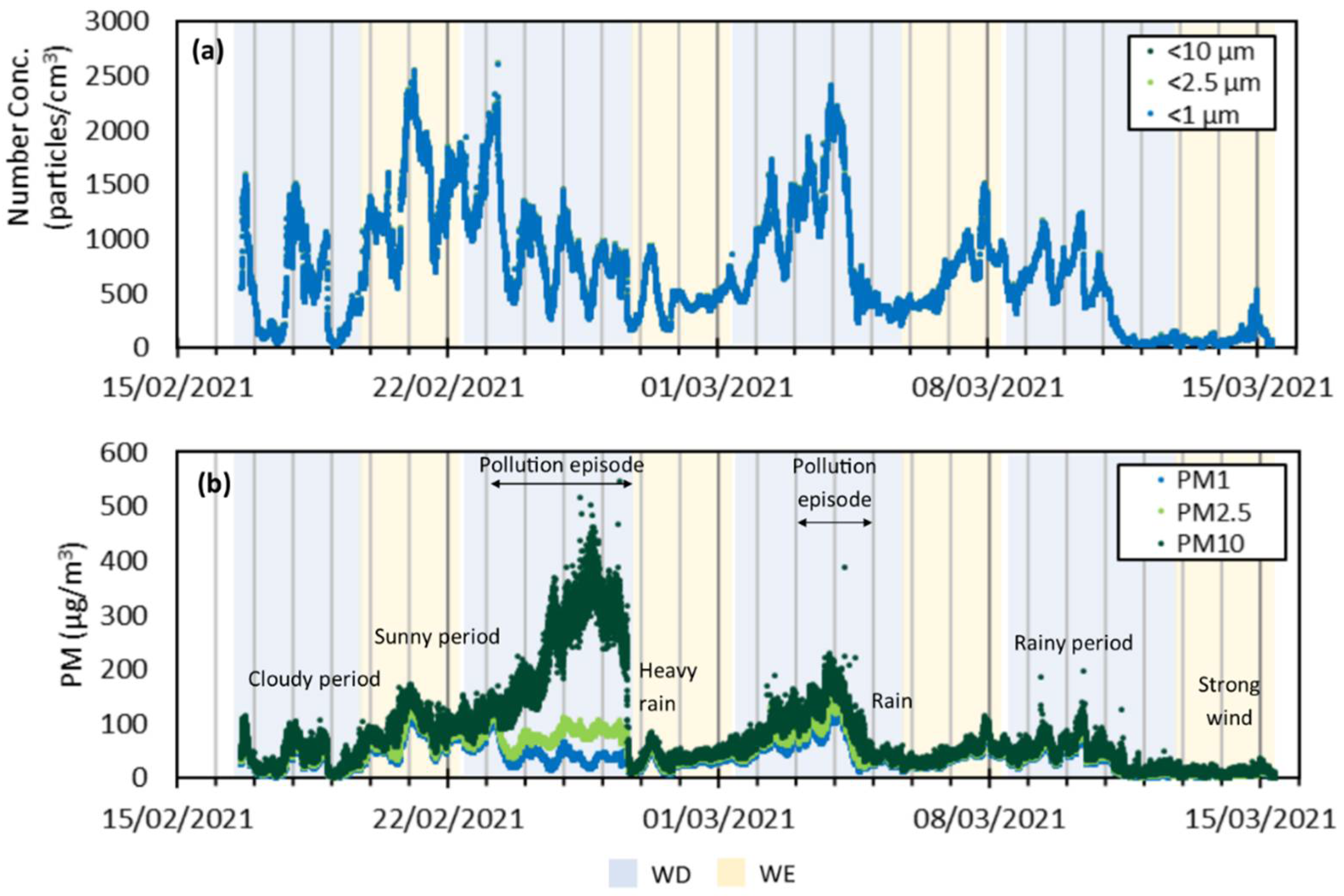
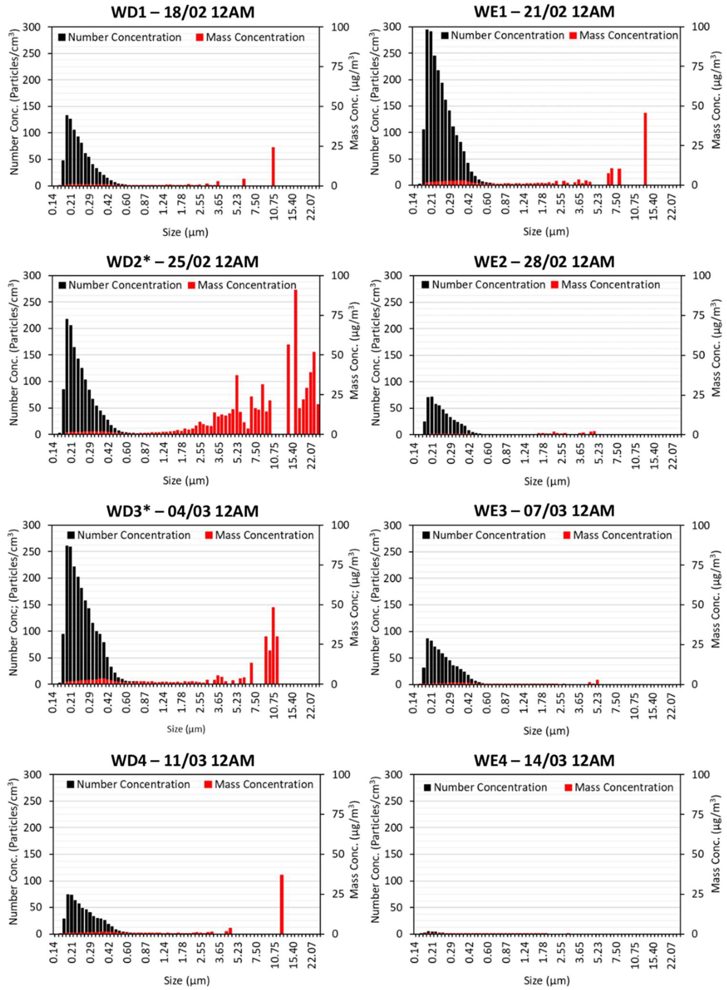
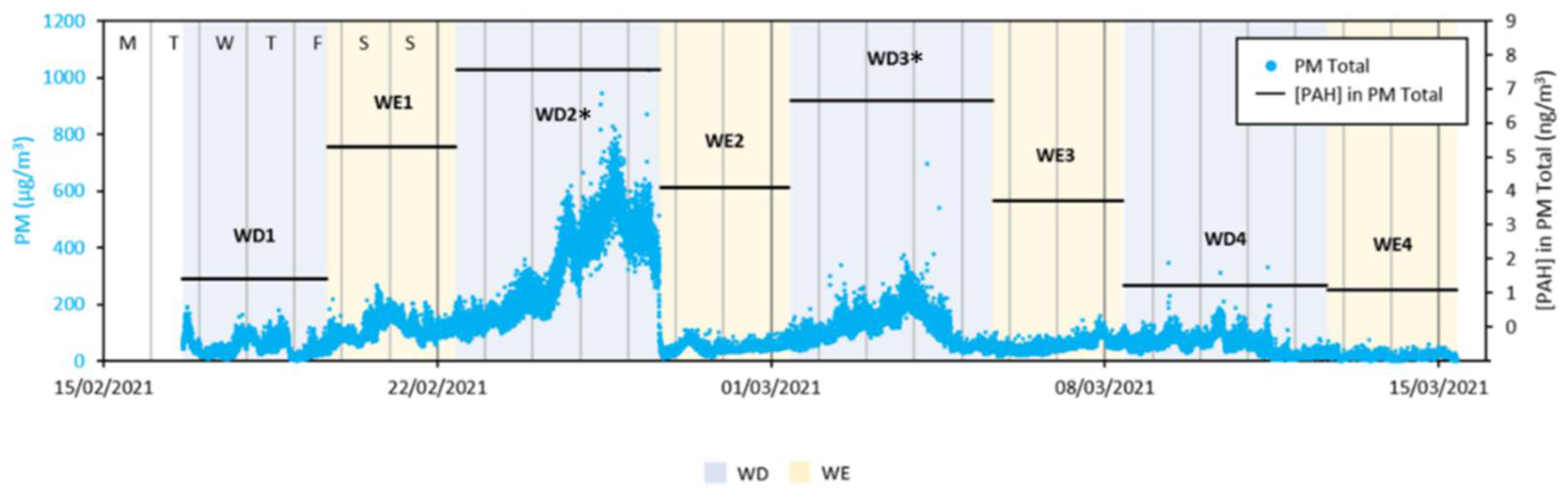
3.1.1. Temporal Variation of PM Concentration

As illustrated in Figure 2, the particle analyser provided the values of particle number concentration and mass concentration corresponding to PM₁, PM_2.5 and PM₁₀ as a function of time.

In terms of number concentration, during the experimental campaign, particles < 1 µm (PM₁), particles < 2.5 µm (PM_2.5) and particles < 10 µm (PM₁₀) were found in concentration ranges of 4.8–2607.6 particles/cm³, 4.9–2613.9 particles/cm³ and 5.0–2614.3 particles/cm³, respectively. In Figure 2a, it is possible to observe that, for particle number concentration, the profiles for PM₁, PM_2.5 and PM₁₀ are overlapped and do not show significant differences. This overlap indicates that the particulate size present in outdoor air is, considering the number of particles, mostly below 1 μm. On the other hand, in terms of mass concentration, PM₁, PM_2.5 and PM₁₀ were in the ranges of 0.3–129.3 µg/m³, 0.4–152.5 µg/m³ and 0.4–547.5 µg/m³, respectively. When looking at the PM values corresponding to mass concentration (Figure 2b), it is visible that the three profiles do not always overlap, and some considerable differences are observed.

During the experimental campaign, two different pollution episodes occurred in Strasbourg: the first between 23 February and 26 February 2021 [20], during WD2, and the second between 3 March and 4 March 2021 [21], during WD3. In both episodes, the reported pollutant was PM₁₀ particles, so an increase of the mass concentration of this PM fraction was expected.

The average PM concentration during WD2 related to this phenomenon was found to be 220.2 µg/m³ for PM₁₀, 78.5 µg/m³ for PM_2.5, and 45.7 µg/m³ for PM₁.

The particle accumulation leading to the pollution episode during WD3 led to an average concentration of 94.3 µg/m³ for PM₁₀, 67.3 µg/m³ for PM_2.5, and 55.4 µg/m³ for PM₁.

After both pollution episodes, there were two distinct precipitation episodes causing a decrease of PM in air which can clearly be observed in Figure 2b, particularly after the first pollution episode at the end of WD2. High precipitation or rainy periods favor the wet deposition of particulate matter because after coming in contact with water droplets, the particles become heavier and settle more easily [22], which explains the decrease in particle mass and number concentrations in air.

The last two periods (WD4 and WE4), particularly between 12 March and 15 March 2021, were characterized by lower concentrations of particulate matter, due to a rainy period followed by strong wind period (see Figure S5), which both contributed to wash away the particles and prevent them from accumulating in the atmosphere.

It is clearly observed that the particulate matter presence in outdoor air is influenced by atmospheric parameters such as rain. With the data recorded with the weather station it was also possible to further study the influence of different meteorological parameters, such as temperature, humidity, wind speed, and solar radiation on the number concentration and dispersion of particles in air. These results can be found in Figure S5. During the sampling period, the maximum and minimum temperatures were 21.8 °C and −0.7 °C, respectively, while the relative humidity varied between 34% and 96%. The maximum wind speed was noted at 5.8 m/s, while the maximum solar radiation was 789 W/m².

With the data provided by the particle analyser, it was also possible to extract the particle size distribution both in number and in mass concentrations for certain times, which are presented in Figure 3. For comparison, a time instant in the middle of each period was selected to further analyse the size distribution (18 February (WD1), 21 February (WE1), 25 February (WD2), 28 February (WE2), 4 March (WD3), 7 March (WE3), 11 March (WD4) and 14 March (WE4)). For all periods, these results were obtained for a time corresponding to midnight (12 AM), chosen considering the higher particle number concentrations obtained at night.

From Figure 3, it can be observed that in number concentration, the particulate matter present in air is mostly below 0.87 μm for all periods and bigger particles are not visible (in terms of number). The total number concentration varied in the ranges 25–2121 and 1–18 particles/cm³ for particles lower and bigger than 0.87 µm, respectively. Regarding the number size distribution, the size range peak is around 0.19–0.22 µm for all the samples. However, in terms of mass concentration, it is noticeable that the main contribution comes from larger particles. This contrast is particularly clear for the periods corresponding to the two pollution episodes (WD2 and WD3).

Furthermore, when comparing the different sampling weeks, it is again clearly shown that the 4th week of sampling had much lower particle concentration, reaching minimum values close to zero for WE4 (0.3 µg/m³ for PM₁ and 0.4 µg/m³ for PM_2.5 and PM₁₀).

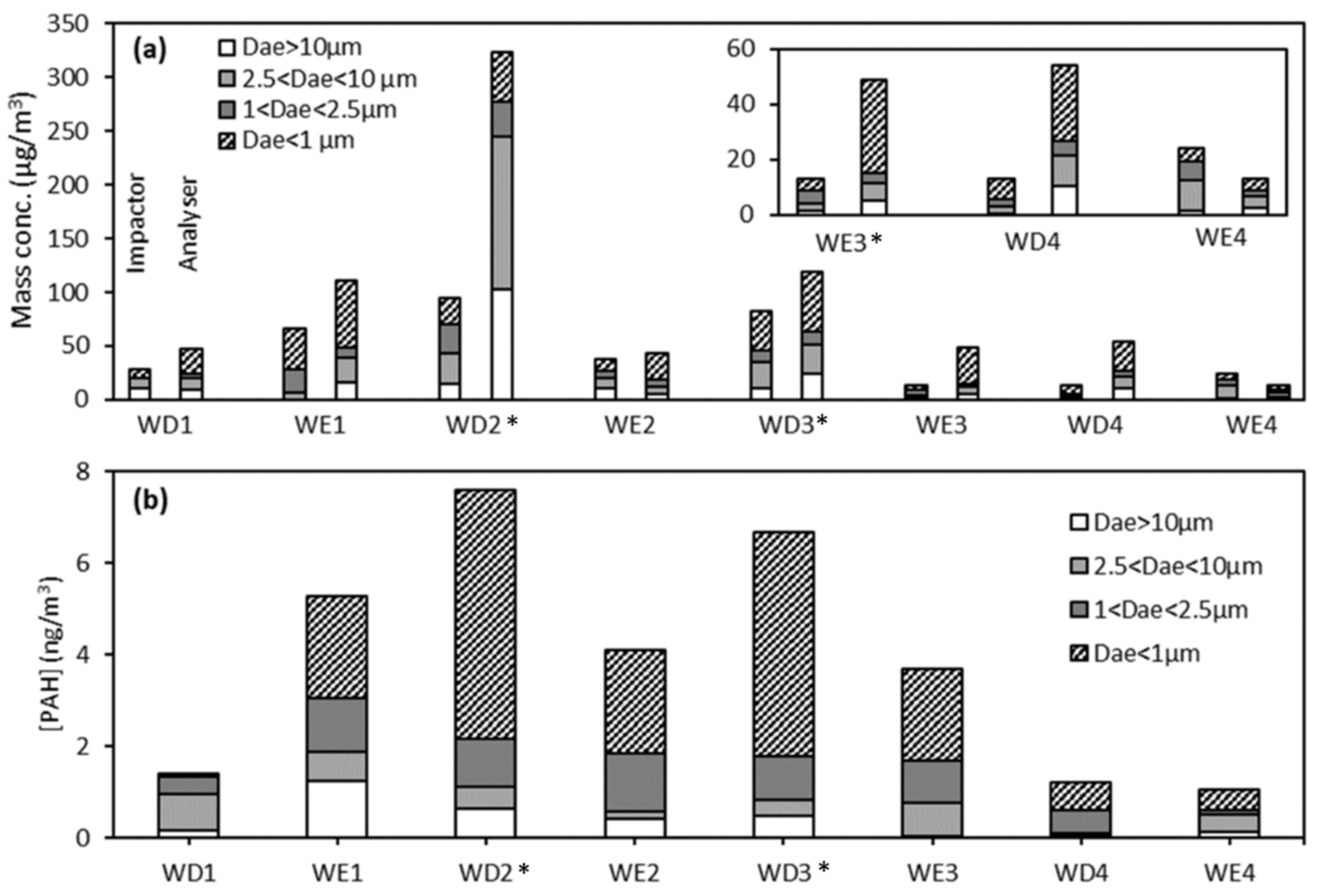
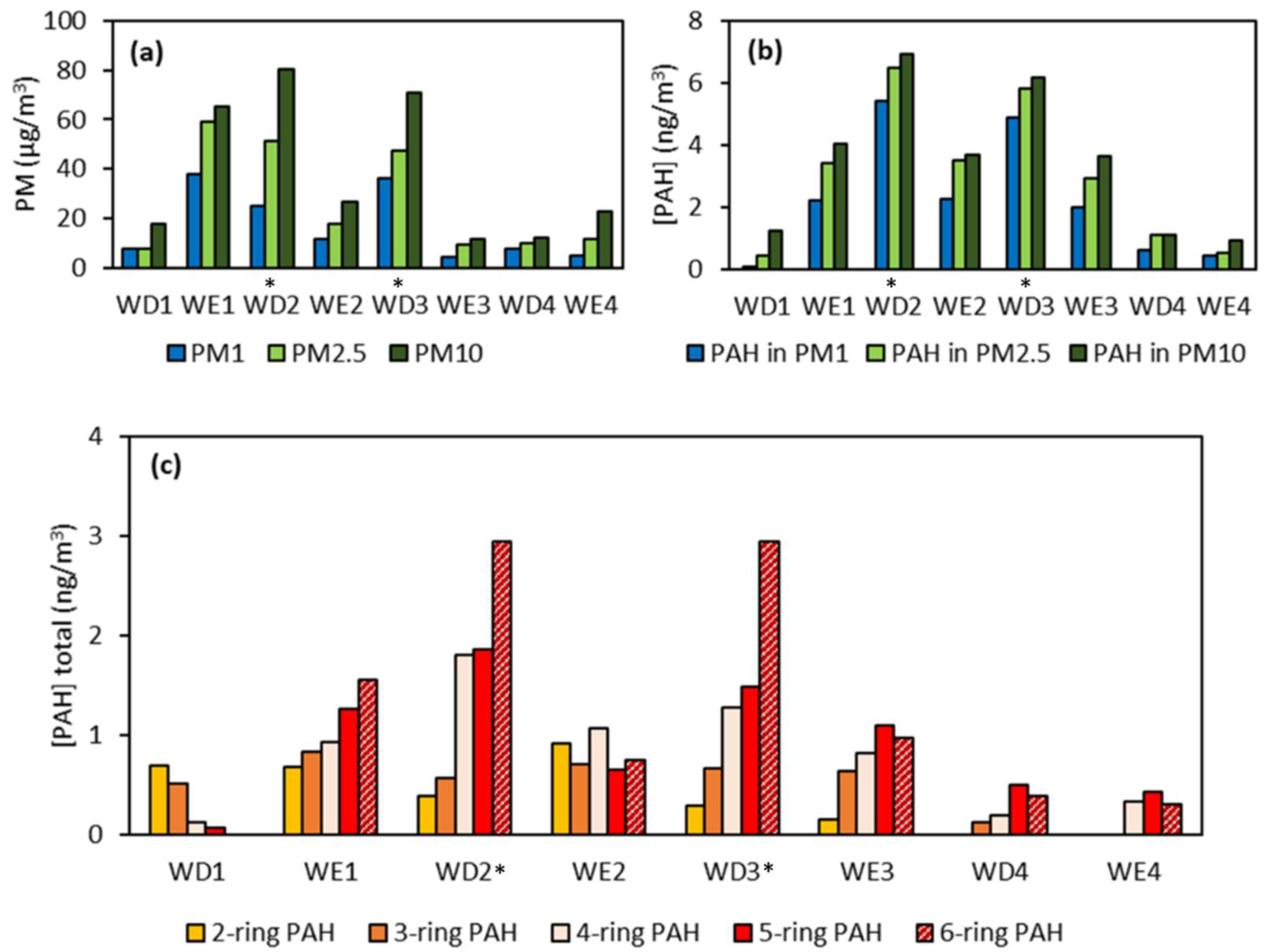
3.1.2. Average PM Concentrations in Air

Table 2. Particle mass concentration in the different size ranges and PM values (µg/m³).

Period	Three-Stage Cascade Impactor DEKATI								Particle Analyser Promo LED 2300 a
	A b	B b	C b	D b	PM1	PM2.5	PM10	PM Total	A b	B b	C b	D b	PM1	PM2.5	PM10	PM Total
WD1	10.6	9.8	0.0	7.9	7.9	7.9	17.7	28.3	9.1	11.1	4.7	21.8	21.8	26.5	37.6	46.7
WE1	0.4	6.1	21.1	37.9	37.9	59.1	65.2	65.6	16.5	22.9	9.2	62.2	62.2	71.4	94.3	110.7
WD2 *	14.6	29.2	25.9	25.2	25.2	51.1	80.2	94.9	102.6	141.7	32.7	45.7	45.7	78.5	220.2	322.8
WE2	11.2	9.0	6.1	11.6	11.6	17.7	26.7	37.9	4.6	7.8	5.9	25.2	25.2	31.0	38.8	43.4
WD3 *	11.3	23.5	11.1	36.2	36.2	47.4	70.9	82.2	24.1	27.0	11.9	55.4	55.4	67.3	94.3	118.4
WE3	1.2	2.7	4.9	4.2	4.2	9.1	11.8	13.0	5.3	6.1	3.6	34.0	34.0	37.7	43.8	49.0
WD4	0.6	2.6	2.2	7.4	7.4	9.6	12.2	12.8	10.4	10.9	5.3	27.6	27.6	32.8	43.7	54.1
WE4	1.2	11.5	6.6	4.7	4.7	11.4	22.9	24.1	2.3	4.3	2.2	4.2	4.2	6.4	10.6	13.0

^a Average values calculated for each period. ^b A: D_ae > 10 µm; B: 10 µm > D_ae > 2.5 µm; C: 2.5 µm > D_ae > 1 µm; D: D_ae > 1 µm. * indicates the sampling period when the pollution episodes occurred.

reports the PM values obtained for each sampling period with the three-stage cascade impactor and the mass of particles in each impactor stage, as well as the average PM values calculated from the temporal distribution obtained with the particle analyser and the mass of particles in the size range corresponding to each impactor plate. The PM total values were also presented in Table 2, and these include the particles > 10 μm for comparison between equipment. Similarly, Figure 4a presents the particle mass concentration corresponding to each size range for the two different types of sampling, i.e., cascade impactor and particle analyser, for all sampling periods.

In terms of the importance of each size range, for both equipment there was a general predominance of the particles with D_ae < 1 μm (PM₁ fraction), ranging from 4.2 µg/m³ to 37.9 µg/m³ for the cascade impactor and between 4.2 µg/m³ and 62.2 µg/m³ for the particle analyser. The other size fractions had lower concentration ranges, which were, for the cascade impactor and particle analyser (in brackets): 0.0–25.9 µg/m³ (2.2–32.7 µg/m³) for 1 < D_ae < 2.5 µm; 1.1–25.9 µg/m³ (6.1–141.7 µg/m³) for 2.5 < D_ae < 10 µm; 0.1–14.6 µg/m³ (4.6–102.6 µg/m³) for D_ae > 10 µm. Again, the WD2 period corresponding to the sand pollution event was an exception to the predominance of particles with size < 1 μm, since the concentration of larger particles was significantly higher, which agrees with the report of the pollution episode by ATMO Grand Est, where PM₁₀ was the major contributor to particulate pollution [23].

Likewise, the PM values are represented in Figure 5a for the cascade impactor. Apart from PM₁ that was already mentioned, PM_2.5 mass concentration was in the ranges 7.9–59.1 µg/m³ and 6.4–78.5 µg/m³ for the cascade impactor and particle analyser, respectively, PM₁₀ mass concentration was in the ranges 11.8–80.2 µg/m³ and 10.6–220.2 µg/m³, and PM Total was 12.8–94.9 µg/m³ and 13.0–322.8 µg/m³.

3.2. Concentration of Particulate-Bound PAHs

3.2.1. Total PAH Concentration

Figure 4b and Figure 5b show the temporal distribution of PAHs in each collection plate and in each PM fraction, respectively, where the total PAH concentration was in the range 1.1–7.6 ng/m³. According to these two figures, PAHs were preferentially bound to the PM₁ fraction for most periods, with 42.3–73.2% of the total PAHs in this fraction. The exception to this observation is WD1, where most total PAHs (56.5%) is bound to particulate matter of sizes between 2.5 and 10 µm.

As displayed in Figure 5b, the temporal variation trend of total PAH concentration also matched the trend of PM mass concentration obtained from cascade impactor (see Figure 5a) and particle analyser (see Figure 2b). The PAH concentration ranged 0.9–6.9 ng/m³ for PM₁₀, 0.4–6.5 ng/m³ for PM_2.5, and 0.1–5.4 ng/m³ for PM₁. Furthermore, comparing the PAHs concentration on the different periods, the highest concentration of PAHs was obtained in WD2 (7.6 ng/m³) and WD3 (6.7 ng/m³), which correspond to the pollution episodes.

Figure 5c shows the total concentration of PAHs grouped by the number of aromatic rings present in each period. For most sampling periods, there was a predominance of 5- and 6-ring PAHs, which are classified as high molecular weight PAHs (HMW-PAHs). These HMW-PAHs account for 34.3% up to 69.3% of the total PAHs. There was an exception which is WD1 where HMW-PAHs only account for 5.1% of total PAHs. LMW-PAHs, which are PAHs with 2 or 3 rings, were present in significant concentrations not only on WD1 but during other sampling periods (12.7% up to 86.3% of the total PAHs), except WD4 and WE4 (10.4% and 0.0% of total PAH concentration, respectively), where pollution levels were low.

In Figure 6, it is possible to further detail the distribution of PAHs grouped by ring in the different PM fractions and collection plate of the cascade impactor. It is clear that 4-ring, 5-ring and 6-ring PAHs are predominantly bound to finer particles (<1 µm), while 2-ring and 3-ring PAHs are generally more evenly distributed between fractions. For some periods, there is even a predominance of LMW-PAHs in coarse particle fractions, such as in WE1, where the fraction of these PAHs in particles with D_ae > 10 µm is of considerable significance (86.3% of total PAH concentration).

Concerning the pollution episodes, a clear increase of the total concentration of 4-, 5- and 6-ring PAHs could be observed during WD2 and WD3, particularly for 6-ring PAHs.

A comparison between the PAH concentrations obtained for each period with the cascade impactor and the temporal profile of PM obtained with the particle analyser was also done. Figure 7 shows the profile for PM Total and the concentration of PAHs in PM Total for the different sampling periods. Similar graphs, obtained for PM₁, PM_2.5 and PM₁₀ with the concentration of PAHs in each PM fraction can be found in Figure S6 of the Supplementary Materials. In Figure 7, it is easily discernible that PAH concentration in air and PM values follow the same trend, with the periods where PM Total was the highest matching the highest PAH concentrations.

Finally, as seen with PM values, the PAH concentration is lower on weekends than on working days, except for WE1 (as discussed before for PM values).

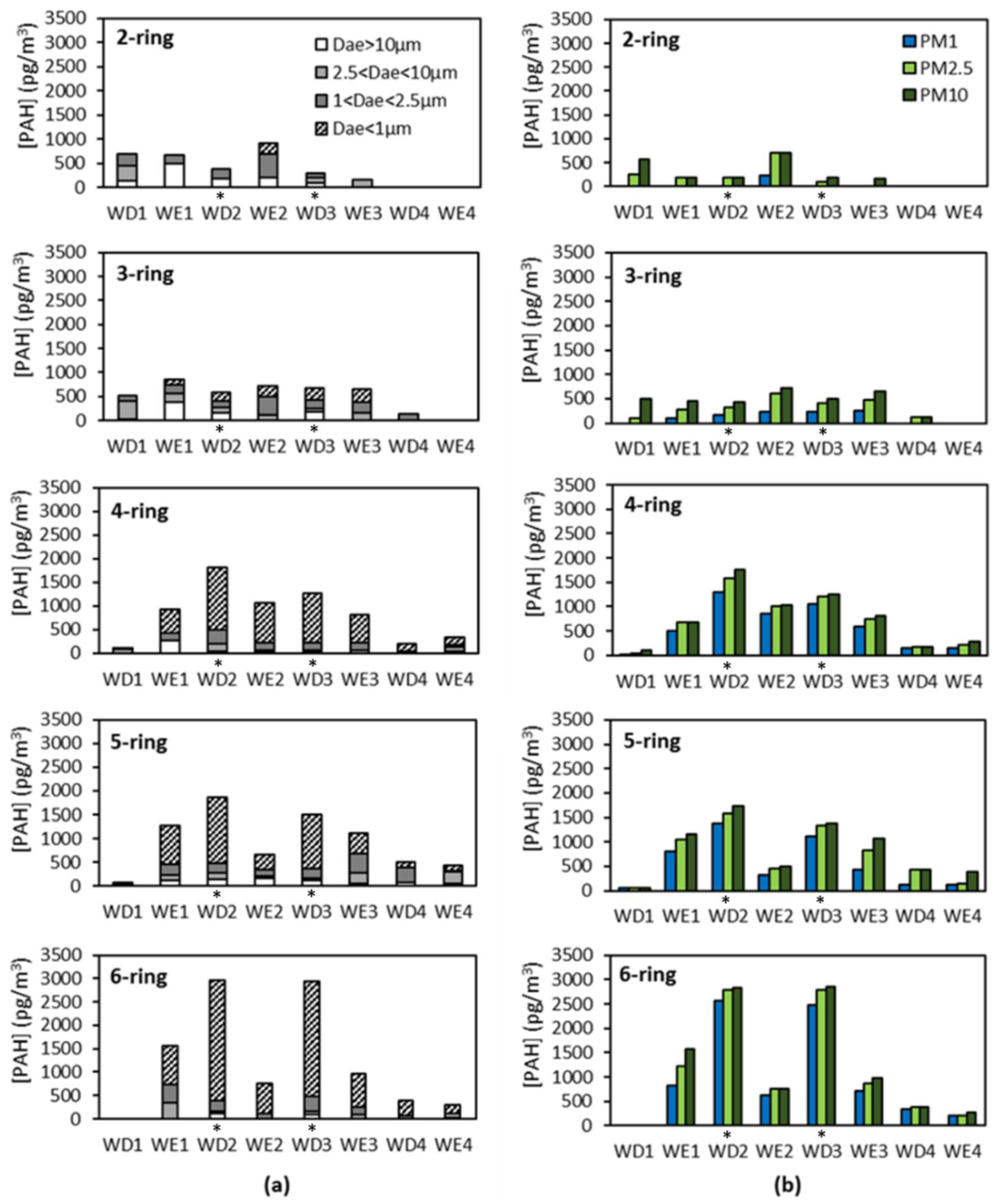
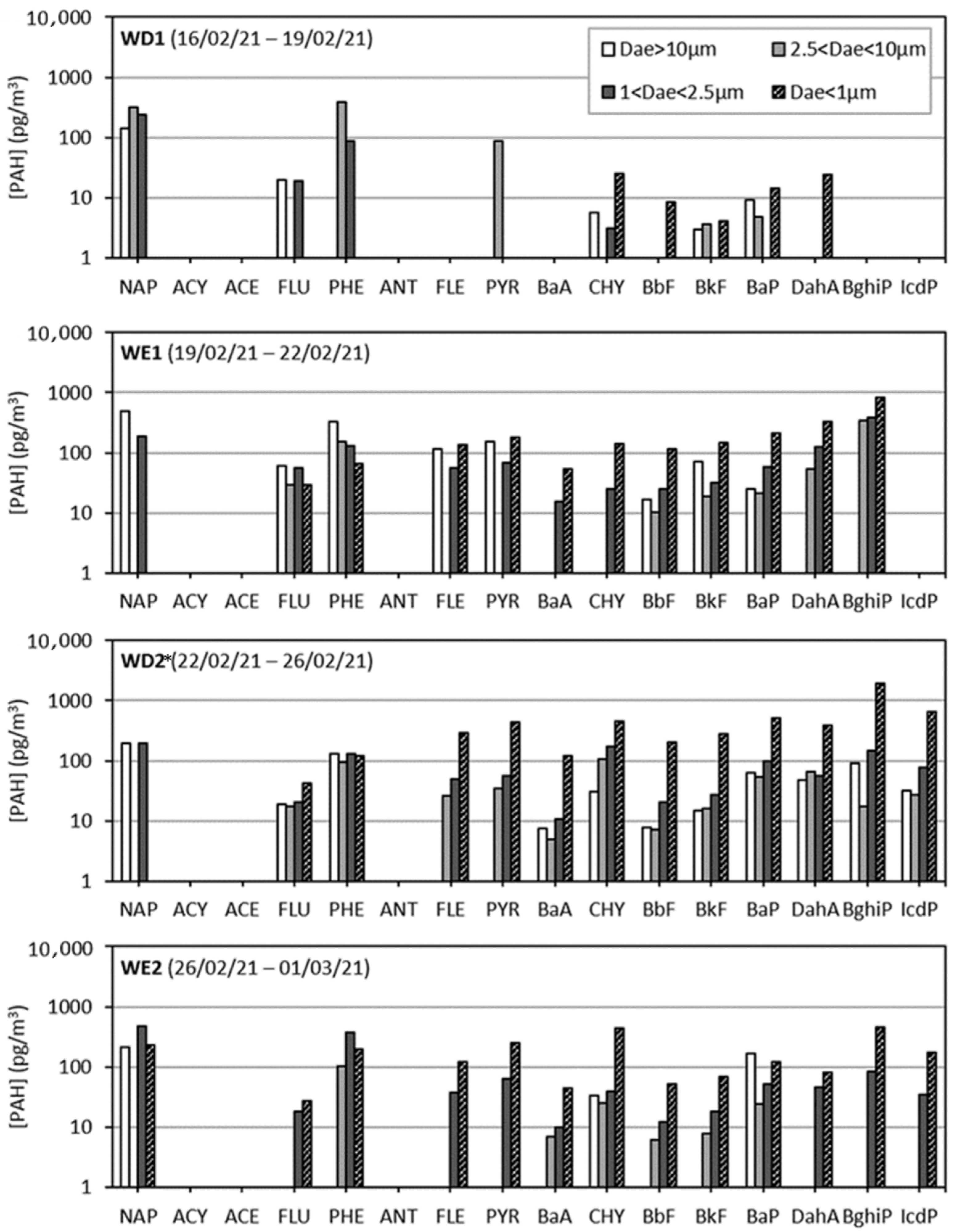
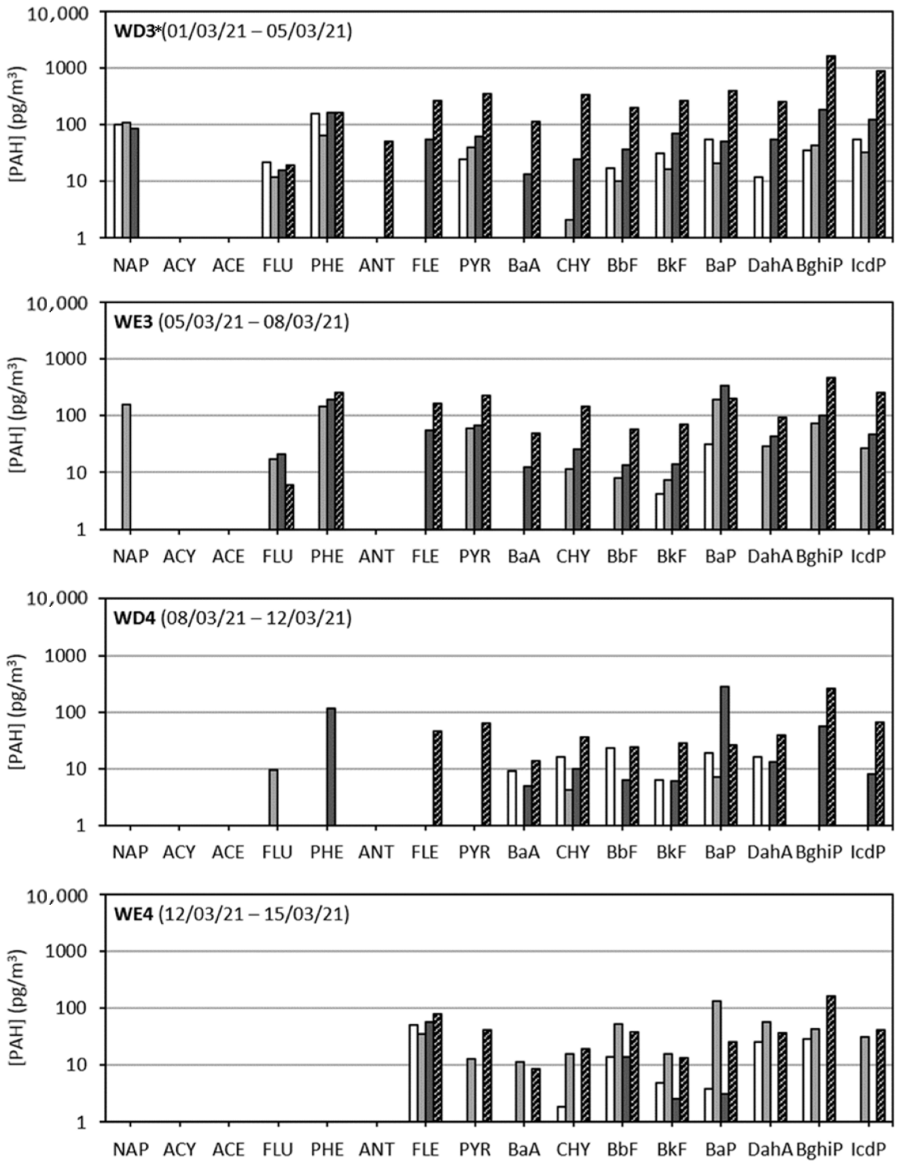
3.2.2. Individual PAH Concentrations

Among the 16 PAHs studied, 14 PAHs were detected during the experimental campaign. ACY and ACE, both LMW-PAHs, were not detected.

Figure 8 shows the distribution of the studied PAHs in the different collection plates for all sampling periods. Similar information for PM fractions instead of collection plates can be found in Figure S7. Logarithmic scale was used for PAH concentration, so that lower concentration values could be read. Additionally, the temporal distribution of individual PAHs during the experimental campaign can be found in Figure S8.

Generally, for all periods of sampling, NAP, FLU and PHE, which are LMW-PAHs, were detected in outdoor environment. PYR and CHY, which are MMW-PAHs, were also found in significant amount, their concentrations varying in the ranges 54.1–524.6 pg/m³ and 33.7–768.7 pg/m³, respectively.

BaP, DahA, BghiP and IcdP were found in high concentrations in the different sampling periods. BaP, the most carcinogenic PAH, was found in concentrations in the range of 28.6 to 762.8 pg/m³. BghiP was the PAH with highest quantities found during the sampling campaign, where the concentrations were in the range of 317.8 pg/m³ up to 2157.7 pg/m³, while DahA and IcdP were found in the ranges 23.9–556.2 pg/m³ and 72.8–1095.2 pg/m³, respectively.

4. Discussion

4.1. Particulate Matter Concentration

4.1.1. Temporal Variation of PM Concentration

As mentioned, there were two different pollution episodes during the experimental campaign: the first during WD2 and the second during WD3. In general, pollution episodes in the city occur due to particle accumulation originated from combustion activities (e.g., transportation and heating) combined with stagnant meteorological conditions (such as the absence of precipitation, lack of wind, etc.) that do not allow the accumulated particles to disperse [10].

The first pollution episode was marked by a special phenomenon of wind bringing sand and dust particles from the Sahara Desert in North Africa to Southern Europe. This pollution episode started from 23 February 2021, where the PM profiles stop overlapping (see Figure 2b) and there was a considerable increase of PM₁₀ when compared to the two other fractions as illustrated by the size distribution displayed in Figure 3 (WD2). This indicated that the dominant size of particles was above 2.5 µm, as confirmed by the mass concentration distribution shown in Figure 3 (WD2), which might be related to Saharan sand and dust particles possibly mixed with another local source of particles. This hypothesis was confirmed by the local observatory of air quality (ATMO Grand Est) which published a statement on the chemical composition of particles proving their pollution source. They reported that Saharan particles corresponded to 41 up to 69% of PM₁₀ mass concentration [23]. Specifically, they reported PM₁₀ mass fractions for the period between 1 February 2021 and 28 February 2021, in terms of elemental carbon, organic matter, nitrate, ammonium, sulfate, sea spray and Saharan particles.

The second pollution episode displayed in Figure 2 and Figure 3 and observed during WD3 was of smaller intensity and was caused mainly by particles coming from combustion activities and spring agricultural activities with some residual particles from the previous Saharan dust wind episode [21]. The particle accumulation leading to the pollution episode was mostly due to sunny and relatively stable atmospheric conditions.

It is important to note that particulate matter concentration in air depends on the multiple meteorological parameters, as well as other factors, such as the seasons and geographical position of the sampling location. Therefore, it is not easy to establish a relation between the different parameters alone and the PM values, but it is possible to observe certain trends. Briefly, from Figure S5, temperature and particle number concentration in air in Strasbourg have an inversely proportional relation, as, generally, lower temperatures lead to higher particle concentration and vice-versa. This might be linked to temperature-related atmospheric phenomena, such as convection currents [22], which are more frequently observed at higher temperatures, creating wind movements that promote the dispersion of particulate matter in air.

In opposition to the impact of temperature, relative humidity is directly proportional to the particle number concentrations, with decrease in relative humidity being accompanied by decrease in particle concentration and vice-versa. High humidity promotes the accumulation of finer particles in the atmosphere and the formation of haze, allowing the particles to rest longer in a certain area and, thus, leading to higher PM values in air [24].

Wind speed is another important parameter to consider because the presence or absence of wind currents can promote the movement or stagnancy of particulate matter in an area [25]. During the sampling period, in general, high wind speeds were related to lower number particle concentration, which means wind promoted the diffusion of the particles to outside the sampling area. This phenomenon is particularly noticeable during the strong wind episode between 11 March and 15 March (at the end of WD4 and during WE4) when extremely low particle concentrations were recorded.

Finally, in terms of solar radiation, the influence on particle number concentration is easily observed during a 24-h period. High solar radiation with minimum clouds during the day generally gives lower PM mass concentration, while low or absence of solar radiation during the night generally gives higher PM mass concentration. This phenomenon is related to either the photolysis of organic fraction of particles by the solar radiation, reducing the PM mass concentration during the day [22], or the upward movement of PM promoted by solar radiations [22].

Furthermore, by looking at the different working days (WD) and the weekend (WE) periods, it is possible observe some differences. With the exception of WE1, both number and mass concentrations are much lower on the WE periods than on the WD ones. This might have occurred because of the curfew measures, since if people were staying home during the weekend, it could result in less traffic and thus less pollution would be expected. However, WE1 was an exception to this trend, which might be a direct consequence of the beginning of the first pollution episode.

4.1.2. Average PM Concentrations in Air

Table 2 and Figure 4a show that the results obtained with the three-stage cascade impactor follow the expected trend, with highest particle concentrations appearing for WE1, as a consequence of the beginning of the first pollution episode, for WD2 due to the same pollution episode, and for WD3, because of to the second pollution episode. It is also confirmed that the presence of particulate matter in air in the 4th week (both WD4 and WE4) was very low. Figure 5a shows the PM values for the cascade impactor, and once again it is clear that the highest PM values were obtained, as expected, for WD2 and WD3.

When comparing the two types of sampling, (see Figure 4a), the values of particles mass concentration obtained with the impactor are usually of the same order of magnitude but lower than those found with the particle analyser. In other words, it is visible that, even though temporarily both follow the same trend, the particle analyser reports higher PM Total values than the three-cascade impactor, particularly during WE1, WD2, WE3 and WD4, with the highest difference appearing for WD2 (322.8 and 94.9 µg/m³, respectively). Multiple factors could be responsible for the highest values given by the particle analyser, such as different size ranges of detection, different methods of sampling, different flow rates, as well as the specificities of the PM algorithm used by the Palas software.

Previous works in the literature have highlighted discrepancies in particle mass concentration between gravimetric methods (such as the three-stage impactor) and real-time particle analysers and reported the existence of clear systematic biases in instruments for real-time particle monitoring [26]. Giorio et al. (2013) concluded that this difference is expected because the optical particle analysers are measuring various types of particles with different refractive indices, shapes and densities that are not accounted for [27]. Thus, an accurate previous calibration should be performed to minimize these biases [27]. However, the PM algorithm used in the Palas software was the environmental version, that was indicated for measurements in outdoor air, and so should account for these variabilities in types of particles.

In fact, the main reason for the highest PM values obtained with the particle analyser could be related to the humidity of air. It has been reported that humidities higher than 80% can lead to overestimation of an aerosol’s mass by real-time particle analysers in comparison to filter-based methods, where most of the water as time to evaporate before the weighing of the filters [28]. In Figure S4, it is visible that relative humidity reached values higher than 80% almost every day during the sampling period, indicating that high humidity could indeed be the main cause for the highest PM values obtained with the particle analyser.

There is one exception to this trend, which is WE4, where the PM Total obtained with the cascade impactor was almost two times higher than the value obtained with the particle analyser. The slightly different locations could also partially explain the observed mass concentrations.

The Directive 2008/50/EC establishes a daily mean limit value of 50 µg/m³ for PM₁₀ that cannot be exceeded more than 35 times a year [3]. Even though the averages presented in Table 2 are based on more than one day, the comparison with this mean value is still interesting to conclude about the air quality in Strasbourg. In fact, for both the cascade impactor and the particle analyser, there are three sampling periods when this limit is surpassed: WE1 (65.2 and 94.3 µg/m³, respectively), WD2 (80.2 and 220.2 µg/m³, respectively) and WD3 (70.9 and 94.3 µg/m³, respectively). As previously discussed, the high PM₁₀ values on these three periods are associated with the PM₁₀ pollution episodes, so it is not surprising to have values higher than the limit level. Pollution episodes caused by natural occurrences, such as windblown desert dust from Africa, sea spray and wildfires, are known for causing the increase of PM₁₀ values above the annual limit established by EU in different countries of Southern and Western Europe (Cyprus, France, Greece, Italy, Portugal, Spain and United Kingdom) [6]. In fact, in Spain, more than 70% of the times that PM₁₀ is above the daily limit mean value in regional background EMEP (European Monitoring and Evaluation Programme) sites, the cause was ascribed to African dust episodes [29]. Outside of these pollution episodes, the daily average PM₁₀ values do not exceed the limit of 50 µg/m³.

On the other hand, in terms of PM_2.5, the annual average of 25 µg/m³ established by the same directive was also surpassed, but the results between two sampling methods were very different. In the case of the cascade impactor, PM_2.5 was higher than the European limit only for WE1, WD2 and WD3, following the same trend of PM₁₀. However, looking at the particle analyser results, the values of PM_2.5 surpass the limit for all periods, except WE4 (when pollution levels were much lower). It is important to take into account that the limit value of the Directive 2008/50/EC was established considering a standard gravimetric method as sampling method [3]. Thus, it is not surprising that the values obtained with the particle analyser are higher than the limit established, because it was observed in this work that the particle analyser generally gives much higher PM values in comparison to the gravimetric three-stage cascade impactor.

Regarding the possible effect of lockdown and the resulting traffic restrictions, ATMO Grand Est reported annual average PM₁₀ value in the order of 22 µg/m³ for 2019, i.e., before the COVID crisis, for the measuring station closest to our sampling site (Boulevard Clemenceau) [30]. Apart from the dust pollution episodes, our PM₁₀ concentrations varied in the range 11.8–22.9 µg/m³ with an average value of 16.1 ± 5.2 µg/m³. This could suggest that the lockdown and traffic reduction could have a positive effect on PM pollution.

4.2. Concentration of Particulate-Bound PAHs

4.2.1. Total PAH Concentration

In Figure 4b and Figure 5b, PAHs were predominantly present to the PM₁ fraction for most periods, with exception of WD1. These results, showing that PAHs are preferentially bound to finer particles, are consistent with those reported in the literature [10,31,32] and confirm the high risk of airborne PAHs to human health through inhalation of fine particles. This tendency for PAHs to be found on finer fractions can be related to the simultaneously generation of PAHs and fine particles during incomplete combustion processes [33] or to the generation of fine particles from the condensation of PAHs from vapor phase [32]. Furthermore, finer particles have higher surface area than bigger particles, which means that they have more surface for the PAHs to be bound to. The presence of PAHs in coarse particles could be explained by the possible agglomeration of fine particles into larger particles or the integration of fine particles into existing larger particles [33].

As PM₁ number concentration is always higher in our study and their specific area are supposed to be greater than those of PM_2.5 and PM₁₀, it is not surprising to observe more PAHs in PM₁ in terms of absolute of mass concentration (µg/m³). It is why it also interesting to compare the normalized PAH concentrations with respect to the particle class fraction. These results can be found in Table S1 and Figure S9. In terms of percentages, normalized values of PAHs in PM₁ were the following: 7% (WD1); 33% (WE1); 50% (WD2); 37% (WE2); 39% (WD3); 43% (WE3); 28% (WD4); 52% (WE4). The PAH distribution shows therefore that PAHs are always abundant in PM₁, particularly for the first Saharan dust episode in WD2, but except for WD1. For PM_2.5 and PM₁₀, their corresponding percentages vary in the ranges 25–41 % and 20–52%, respectively, indicating a homogeneous distribution when normalized concentrations are considered. WE3 exhibits the higher normalized PAH concentration in all PMs, which was not expected considering this is not during the pollution episodes. High humidity and low solar radiation during the whole day on Friday 05/03, and suddenly lower temperatures reached on WE3 were observed (see Figure S5). Because of these atmospheric conditions, PAHs could have been first accumulated in the atmosphere and then adsorbed by the particles in air.

The highest concentration of PAHs was obtained in WD2 and WD3, which correspond to the pollution episodes. This is consistent with the observations made by the local observatory of air quality [23] since they reported an increase of organic matter and black carbon for the first pollution episode, i.e., from 23 February to 26 February 2021. In fact, these increases started from Saturday 20 February which corresponds to the beginning of the Saharan dust episode observed in our sample WE1 (see Figure 3 and Figure 4b). As Saharan dust is known for being a carrier of anthropogenic pollutants and micro-organisms [29], contributing to the increase of these pollutants, it can explain the higher occurrence and higher concentration of PAHs in PM. However, this is the first time that PAHs concentrations were evaluated and reported during a dust episode simultaneously with limited anthropogenic activities due to the unique COVID confinement.

Figure 5c shows that, generally, there was a predominance HMW-PAHs, indicating that particulate-bound PAHs are predominantly HMW-PAHs. To understand these results, it is important to consider that PAHs in air can be found either in vapor phase or in particulate-bound phase. The distribution of PAHs between these two phases is dependent on their vapor pressure. PAHs with lower vapor pressure, which correspond to HMW-PAHs, tend to be bound to particles, while PAHs with higher vapor pressure, which are those with low molecular weight (LMW-PAHs) are typically associated with vapor phase although this may be less the case at low temperatures during winter. PAHs with intermediary molecular weights (MMW-PAHs) are more evenly distributed between the two phases [34]. For this reason, MMW- and HMW-PAHs were likely to be detected in PM, as opposed to LMW-PAHs. Thus, the observed presence of LMW-PAHs in PM was not expected since these PAHs are normally found on vapor phase. These results will be further debated when individual PAH concentrations are discussed (see below).

As seen in Figure 6, 4-ring, 5-ring and 6-ring PAHs are predominantly bound the PM₁ fraction, while 2-ring and 3-ring PAHs are more uniformly distributed between fractions, which is in agreement with previous studies [10,31]. However, it is interesting to see that for some periods, such as WE1, LMW-PAHs are predominantly in coarse particle fractions (D_ae > 10 µm). One explanation for this observation is that due to the higher vapor pressure of LMW-PAHs, they evaporate easily from fine particles and are then adsorbed into larger particles, while the HMW-PAHs would require much longer times to evaporate and be adsorbed by larger particles and, thus, remain in finer fractions [33,35]. Additionally, it is also possible that there is more chemical affinity between LMW-PAHs and coarse particles, and between MMW- and HMW-PAHs and finer particles [35], depending on the particles’ source and composition.

There is also a clear increase of concentration of 4-,5- and 6-ring PAHs during the periods of the pollution episodes (WD2 and WD3), in particular for 6-ring PAHs. This increase in concentration was largely caused by the increase in concentration of the PAHs in PM₁ fraction. It is interesting to note that, for 2- and 3-ring PAHs, there was no increase of concentration for the pollution episode periods, and there was even a decrease for WD2 and WD3 when compared to WE1 and WE2, respectively. For WD2, the observed increase of temperature up to 20.1–21.8 °C for 3 consecutive days could promote the evaporation of LMW-PAHs into the gas phase, limiting their PM concentration.

On the other hand, in Figure 7, it is visible that PAH concentration in air and PM values of the particles analyser generally follow the same trend. This is expected since the PAHs being studied are particulate-bound, so an increase of particle concentration is expected to lead to an increase in PAHs level. However, the PAH and PM did not increase to the same extent. For example, between WD1 and WE1, PAH concentration increases significantly, PM Total mass concentration does not change significantly; however, the PM₁ number concentrations increased (see Figure 2a) which could explain the PAHs concentration increase as they are usually bound with finer particles [31,36] in absence of Saharan dust event.

Lastly, there are generally lower PAH concentrations on weekends than on working days, which might be a direct consequence of the movement restrictions of the curfew measures in place at the time. Vehicular emission is one of the anthropogenic sources of PAHs so, in fact, the decrease in concentration for the weekends might be caused by a decrease in people movement and, thus, vehicular emission of PAHs, which could be an indication that this is the main source of PAHs near the sampling location.

4.2.2. Individual PAH Concentration

16 PAHs were studied during the experimental campaign and of those, 2 were not detected: ACY and ACE, both LMW-PAHs. This is not surprising considering they are both expected to be predominantly in vapor phase instead of being bound to PMs.

NAP, FLU and PHE, which are also LMW-PAHs, were unexpectedly detected in outdoor environment throughout the experimental campaign. This was not expected, at least not in significant concentrations since they have more affinity to vapor phase and not particulate matter. In fact, these results do not agree with previous results reported in the literature for the same type of sampling and quantification [36], where in, an experimental campaign in Mauberge, France, no NAP and much lower concentrations of FLU and PHE were detected in outdoor air. This, coupled with the fact that they were present in almost all sampling periods, might indicate a local source of these three PAHs. LMW-PAHs can be generated from vehicle emissions, waste incinerators and steel iron plants [10]. Furthermore, NAP can be used outside for pest control in gardens [37], which could be a possibility for its source, if it is present in pesticides used near our sampling site.

PYR and CHY, both MMW-PAHs, were also detected in significant amount. PYR is considered to be related to emission from diesel vehicles, while CHY usually comes from biomass-related combustions (e.g., wood, food, garbage) [38]. A specific increase of CHY concentration was observed on the WD2 which may be related to the first pollution episode. The Saharan dust particles could have been responsible for bringing this PAH from other areas that they pass through.

The four PAHs with highest molecular weight (BaP, DahA, BghiP and IcdP) were present in high amount during the experimental campaign. These compounds are generally associated with pollution from vehicle emission in traffic in highways or urban areas [39] and so, the proximity to main roads and highways could explain the presence of these pollutants outside the pollution episodes.

It is also important to note that BaP, the most carcinogenic PAH, was found in quantities lower than the annual average limit established by European Union, which is 1 ng/m³. Furthermore, ATMO Grand Est has reported the concentration of BaP in Strasbourg (Boulevard Clemenceau) in 2018 with daily concentrations varying between 0.02 and 0.85 ng/m³ throughout the year [40], which led to an annual average of 0.2 ng/m³. As previously mentioned, the BaP concentration ranged from 28.6 to 762.8 pg/m³ (≈0.03 to ≈0.76 ng/m³) during our experimental campaign, which are in the same order of magnitude than those obtained of 2018. This indicates that COVID restrictions did not have a significant impact in BaP concentration.

4.2.3. Health Risk Assessment Due to PAH Exposure

It is possible to estimate the carcinogenic risk due to PAH exposure for the different periods of the sampling campaign. This is done by calculating the BaP equivalent factor (BaP_eq). To obtain this equivalent factor, the Toxic Equivalency Factor (TEF) that estimates the relative carcinogenic potency of each PAH relative to the carcinogenicity of BaP is used [31,41]. This means that a certain BaP_eq value has the same carcinogenic effect as if BaP was present in that same concentration.

The TEF values have been determined in previous studies and are specific depending on the carcinogenicity of each PAH. The BaP_eq is then calculated as the sum of each PAH concentration multiplied by the respective TEF [31,41]. The TEF values used were reported in Nisbet & LaGoy (2012) [41], choosing a TEF of 1 for DahA, because it is considered to be present in high concentration.

The BaP_eq values (Table S2) varied between 56.1 and 1462.5 pg/m³ (≈0.06 to ≈1.46 ng/m³). These BaP_eq values surpassed the annual EU target value for BaP (1 ng/m³) two times during the experimental campaign in the periods corresponding to the pollution episodes: in WD2, BaP_eq reached the maximum value of 1.46 ng/m³, and in WD3 it reached 1.06 ng/m³. The target value of the EU was established to minimize the effects on human health [4], so the the BaP_eq values obtained during the pollution episodes can be worrying. However, it is important to consider that these values correspond to weekly averages, while the target value was established for one entire year.

5. Conclusions

The three-stage cascade impactor and the particle analyser were successful in monitoring PM, according to their particle size, in outdoor environment. A comparison between three-stage cascade impactor DEKATI and Palas particle analyser showed that the particle mass concentration followed the same general behavior. However, the values recorded by the particle analyser, i.e., for total PM, were usually 144–422 % higher than those found with the impactor. Note that the conclusions might be sometimes taken with caution as the measurements were not replicated, which also makes it difficult to estimate the measurement uncertainties.

PAHs concentration trend was found to be similar to PM concentration one which indicates the link between the two. PAHs were observed to be more abundant in PM₁ and the main PAHs were HMW-PAHs (5- to 6-ring). 14 PAHs were found during the sampling campaign, with the most significant being NAP, PHE, PYR, CHY, BaP, DahA, BghiP, and IcdP. BaP, as the most carcinogenic PAH among the sixteen, was found in concentration range below the European annual mean target of 1 ng/m³. The presence of these PAHs suggested that vehicular emission was one of the main sources of PAHs in air in Strasbourg during the sampling campaign even though people’s movements were limited after 6 PM due to COVID crisis.

The temperature and solar radiation were found to be inversely proportional to the daily PM concentration during the sampling period in Strasbourg, while the relative humidity was directly proportional. Precipitation and wind speed also played important roles modifying the PM concentration by introducing or sweeping away particles in the air.

The period of the sampling campaign included two pollution episodes in Strasbourg, particularly a Saharan dust wind episode. It is worth mentioning that to the best of our knowledge, there are no works published in the literature that quantified simultaneously the PM and PAHs bound to PM of Saharan dust yet. The pollution episodes, especially the one associated with Saharan dust in WD2, led to significantly higher PAH and PM concentrations during the WE1, WD2 and WD3, with PM₁₀ and PM_2.5 substantially exceeding the EU daily limit of 50 µg/m³ and 25 µg/m³, respectively, in a context of low car traffic favored by the COVID restrictions. Therefore, it is not excluded that PAHs could be bound to sand particles and could have been carried by these same PM far away from their emission sources. Whatever the case, such observation of an exceedance of the PM threshold values is cause for concern and suggests that particulate pollution is becoming more and more worrying in a context of increasing urbanization of large French and European cities. The exhaust-free vehicles such as fully electric ones, which currently represent only a marginal part of the vehicle fleet, may help to reduce tailpipe emissions but will continue to contribute to particle emissions through tires and road surface wear.

In the future, it would be interesting to extensively characterize the particulate matter from Saharan dust pollution episodes, to better understand the relation between the Saharan sand and PAHs. This characterization could also be complemented with the further study and quantification of other pollutants carried by the Saharan particles in order to fully assess the negative effects of these dust events on human health.

References

1. Leung, D.Y.C. Outdoor-Indoor Air Pollution in Urban Environment: Challenges and Opportunity. Front. Environ. Sci. 2015, 2, 69. [Google Scholar] [CrossRef]
2. World Health Organization (Ed.) Air Quality Guidelines: Global Update 2005: Particulate Matter, Ozone, Nitrogen Dioxide, and Sulfur Dioxide; World Health Organization: Copenhagen, Denmark, 2006; ISBN 978-92-890-2192-0. [Google Scholar]
3. CEC Directive 2008/50/EC of the European Parliament and of the Council of 21 May 2008 on Ambient Air Quality and Cleaner Air for Europe. Off. J. Eur. Union 2008, L152, 1–44.
4. CEC Directive 2004/107/EC of the European Parliament and of the Council of 15 December 2004 Relating to Arsenic, Cadmium, Mercury, Nickel and Polycyclic Aromatic Hydrocarbons in Ambient Air. Off. J. Eur. Union 2004, L23, 316.
5. Marco, G.; Bo, X. Air Quality Legislation and Standards in the European Union: Background, Status and Public Participation. Adv. Clim. Chang. Res. 2013, 4, 50–59. [Google Scholar] [CrossRef]
6. Viana, M.; Pey, J.; Querol, X.; Alastuey, A.; de Leeuw, F.; Lükewille, A. Natural Sources of Atmospheric Aerosols Influencing Air Quality across Europe. Sci. Total Environ. 2014, 472, 825–833. [Google Scholar] [CrossRef]
7. Kim, K.-H.; Kabir, E.; Kabir, S. A Review on the Human Health Impact of Airborne Particulate Matter. Environ. Int. 2015, 74, 136–143. [Google Scholar] [CrossRef] [PubMed]
8. Rodríguez, S.; Querol, X.; Alastuey, A.; de la Rosa, J. Atmospheric Particulate Matter and Air Quality in the Mediterranean: A Review. Environ. Chem. Lett. 2007, 5, 1–7. [Google Scholar] [CrossRef]
9. Kuklinska, K.; Wolska, L.; Namiesnik, J. Air Quality Policy in the U.S. and the EU—A Review. Atmos. Pollut. Res. 2015, 6, 129–137. [Google Scholar] [CrossRef]
10. Dat, N.-D.; Chang, M.B. Review on Characteristics of PAHs in Atmosphere, Anthropogenic Sources and Control Technologies. Sci. Total Environ. 2017, 609, 682–693. [Google Scholar] [CrossRef]
11. Mojiri, A.; Zhou, J.L.; Ohashi, A.; Ozaki, N.; Kindaichi, T. Comprehensive Review of Polycyclic Aromatic Hydrocarbons in Water Sources, Their Effects and Treatments. Sci. Total Environ. 2019, 696, 133971. [Google Scholar] [CrossRef]
12. Zhang, L.; Yang, L.; Zhou, Q.; Zhang, X.; Xing, W.; Wei, Y.; Hu, M.; Zhao, L.; Toriba, A.; Hayakawa, K.; et al. Size Distribution of Particulate Polycyclic Aromatic Hydrocarbons in Fresh Combustion Smoke and Ambient Air: A Review. J. Environ. Sci. 2020, 88, 370–384. [Google Scholar] [CrossRef] [PubMed]
13. Dimashki, M.; Lim, L.H.; Harrison, R.M.; Harrad, S. Temporal Trends, Temperature Dependence, and Relative Reactivity of Atmospheric Polycyclic Aromatic Hydrocarbons. Environ. Sci. Technol. 2001, 35, 2264–2267. [Google Scholar] [CrossRef] [PubMed]
14. He, J.; Fan, S.; Meng, Q.; Sun, Y.; Zhang, J.; Zu, F. Polycyclic Aromatic Hydrocarbons (PAHs) Associated with Fine Particulate Matters in Nanjing, China: Distributions, Sources and Meteorological Influences. Atmos. Environ. 2014, 89, 207–215. [Google Scholar] [CrossRef]
15. Querol, X.; Pérez, N.; Reche, C.; Ealo, M.; Ripoll, A.; Tur, J.; Pandolfi, M.; Pey, J.; Salvador, P.; Moreno, T.; et al. African Dust and Air Quality over Spain: Is It Only Dust That Matters? Sci. Total Environ. 2019, 686, 737–752. [Google Scholar] [CrossRef]
16. Nouvelle Remontée de Sable du Sahara sur la France—Actualités La Chaîne Météo. Available online: https://actualite.lachainemeteo.com/actualite-meteo/2021-03-01/nouvelle-remontee-de-sable-du-sahara-sur-la-france-58539 (accessed on 14 July 2022).
17. Épisodes de Pollution|ATMO Grand Est. Available online: http://www.atmo-grandest.eu/episodes-de-pollution (accessed on 14 July 2022).
18. L’Alsace en Vigilance Jaune Vent Violent, Des Rafales de 100 km/h Attendues en Plaine. Available online: https://www.francebleu.fr/infos/meteo/l-alsace-toujours-en-vigilance-jaune-vent-violence-1615556378 (accessed on 14 July 2022).
19. Liaud, C.; Millet, M.; Le Calvé, S. An Analytical Method Coupling Accelerated Solvent Extraction and HPLC-Fluorescence for the Quantification of Particle-Bound PAHs in Indoor Air Sampled with a 3-Stages Cascade Impactor. Talanta 2015, 131, 386–394. [Google Scholar] [CrossRef]
20. Atmo Grand Est Episode de Pollution de l’air Dans le Grand Est, Polluant PM10, 25 Février 2021. Available online: http://www.atmo-grandest.eu/data/statements/20210225/ATMO_GrandEst_Alerte_PM10_C1_20210225.pdf (accessed on 4 July 2022).
21. Atmo Grand Est Episode de Pollution de l’air dans le Grand Est, Polluant PM10, 03 Mars 2021. Available online: http://www.atmo-grandest.eu/data/statements/20210303/ATMO_GrandEst_Alerte_PM10_C1_20210303.pdf. (accessed on 4 July 2022).
22. Chen, Z.; Chen, D.; Zhao, C.; Kwan, M.; Cai, J.; Zhuang, Y.; Zhao, B.; Wang, X.; Chen, B.; Yang, J.; et al. Influence of Meteorological Conditions on PM2.5 Concentrations across China: A Review of Methodology and Mechanism. Environ. Int. 2020, 139, 105558. [Google Scholar] [CrossRef]
23. Atmo Grand Est Note Sur L’Impact Des Particules Sahariennes Sur Les Niveaux Particulaires de Février 2021 (ENJEM-EN-040). Available online: http://www.atmo-grandest.eu/actualite/sable-du-sahara-quel-constat-sur-la-qualite-de-lair (accessed on 14 July 2022).
24. Zhang, L.; Cheng, Y.; Zhang, Y.; He, Y.; Gu, Z.; Yu, C. Impact of Air Humidity Fluctuation on the Rise of PM Mass Concentration Based on the High-Resolution Monitoring Data. Aerosol Air Qual. Res. 2017, 17, 543–552. [Google Scholar] [CrossRef]
25. Li, J.; Chen, H.; Li, Z.; Wang, P.; Cribb, M.; Fan, X. Low-Level Temperature Inversions and Their Effect on Aerosol Condensation Nuclei Concentrations under Different Large-Scale Synoptic Circulations. Adv. Atmos. Sci. 2015, 32, 898–908. [Google Scholar] [CrossRef]
26. Wang, Z.; Calderón, L.; Patton, A.P.; Sorensen Allacci, M.; Senick, J.; Wener, R.; Andrews, C.J.; Mainelis, G. Comparison of Real-Time Instruments and Gravimetric Method When Measuring Particulate Matter in a Residential Building. J. Air Waste Manag. Assoc. 2016, 66, 1109–1120. [Google Scholar] [CrossRef]
27. Giorio, C.; Tapparo, A.; Scapellato, M.L.; Carrieri, M.; Apostoli, P.; Bartolucci, G.B. Field Comparison of a Personal Cascade Impactor Sampler, an Optical Particle Counter and CEN-EU Standard Methods for PM10, PM2.5 and PM1 Measurement in Urban Environment. J. Aerosol Sci. 2013, 65, 111–120. [Google Scholar] [CrossRef]
28. Wallace, L.A.; Wheeler, A.J.; Kearney, J.; Van Ryswyk, K.; You, H.; Kulka, R.H.; Rasmussen, P.E.; Brook, J.R.; Xu, X. Validation of Continuous Particle Monitors for Personal, Indoor, and Outdoor Exposures. J. Expo. Sci. Environ. Epidemiol. 2011, 21, 49–64. [Google Scholar] [CrossRef] [PubMed]
29. Karanasiou, A.; Moreno, N.; Moreno, T.; Viana, M.; de Leeuw, F.; Querol, X. Health Effects from Sahara Dust Episodes in Europe: Literature Review and Research Gaps. Environ. Int. 2012, 47, 107–114. [Google Scholar] [CrossRef] [PubMed]
30. Atmo Grand Est Bilan Qualité de l’air Bas-Rhin 2020. Available online: http://www.atmo-grandest.eu/document/2636 (accessed on 24 August 2022).
31. Liaud, C.; Dintzer, T.; Tschamber, V.; Trouve, G.; Le Calvé, S. Particle-Bound PAHs Quantification Using a 3-Stages Cascade Impactor in French Indoor Environments. Environ. Pollut. 2014, 195, 64–72. [Google Scholar] [CrossRef] [PubMed]
32. Junyapoon Size Distributions of Particulate Matter and Particle-Bound Polycyclic Aromatic Hydrocarbons and Their Risk Assessments during Cable Sheath Burning. Curr. Appl. Sci. Technol. 2019, 19, 140153. [CrossRef]
33. Allen, J.O.; Dookeran, N.M.; Smith, K.A.; Sarofim, A.F.; Taghizadeh, K.; Lafleur, A.L. Measurement of Polycyclic Aromatic Hydrocarbons Associated with Size-Segregated Atmospheric Aerosols in Massachusetts. Environ. Sci. Technol. 1996, 30, 1023–1031. [Google Scholar] [CrossRef]
34. Abdel-Shafy, H.I.; Mansour, M.S.M. A Review on Polycyclic Aromatic Hydrocarbons: Source, Environmental Impact, Effect on Human Health and Remediation. Egypt. J. Pet. 2016, 25, 107–123. [Google Scholar] [CrossRef]
35. Zhu, Y.; Yang, L.; Yuan, Q.; Yan, C.; Dong, C.; Meng, C.; Sui, X.; Yao, L.; Yang, F.; Lu, Y.; et al. Airborne Particulate Polycyclic Aromatic Hydrocarbon (PAH) Pollution in a Background Site in the North China Plain: Concentration, Size Distribution, Toxicity and Sources. Sci. Total Environ. 2014, 466–467, 357–368. [Google Scholar] [CrossRef] [PubMed]
36. Liaud, C.; Chouvenc, S.; Le Calvé, S. Simultaneous Monitoring of Particle-Bound PAHs Inside a Low-Energy School Building and Outdoors over Two Weeks in France. Atmosphere 2021, 12, 108. [Google Scholar] [CrossRef]
37. Price, P.S.; Jayjock, M.A. Available Data on Naphthalene Exposures: Strengths and Limitations. Regul. Toxicol. Pharmacol. 2008, 51, 15–21. [Google Scholar] [CrossRef] [PubMed]
38. Galán-Madruga, D.; Terroba, J.M.; dos Santos, S.G.; Úbeda, R.M.; García-Cambero, J.P. Indoor and Outdoor PM10-Bound PAHs in an Urban Environment. Similarity of Mixtures and Source Attribution. Bull. Environ. Contam. Toxicol. 2020, 105, 951–957. [Google Scholar] [CrossRef]
39. Liu, S.; Xia, X.; Yang, L.; Shen, M.; Liu, R. Polycyclic Aromatic Hydrocarbons in Urban Soils of Different Land Uses in Beijing, China: Distribution, Sources and Their Correlation with the City’s Urbanization History. J. Hazard. Mater. 2010, 177, 1085–1092. [Google Scholar] [CrossRef] [PubMed]
40. Atmo Grand Est Surveillance Réglementaire Des Hydrocarbures Aromatiques Polycycliques Dans l’air Ambiant Site “Clémenceau”—Valeurs Des 12 Derniers Mois En Date Du 31/12/18. Available online: http://www.atmo-grandest.eu/sites/prod/files/2019-03/Bulletin_trimestriel_HAP_Clemenceau_122018.pdf (accessed on 24 August 2022).
41. Nisbet, I.C.T.; LaGoy, P.K. Toxic Equivalency Factors (TEFs) for Polycyclic Aromatic Hydrocarbons (PAHs). Regul. Toxicol. Pharmacol. 1992, 16, 290–300. [Google Scholar] [CrossRef]
Figure 1. Location and pictures of the experiment sampling sites and different equipment: (a) Cronenbourg campus; (b) ECPM rooftop (three-stage cascade impactor sampling site, weather station location); (c) ICPEES (particle analyser sampling site); (d) three-stage cascade impactor (DEKATI); (e) weather station; (f) particle analyser Palas Promo LED 2300.
Atmosphere 13 01435 g001
Figure 2. Temporal distribution of particle concentration in air during the sampling period, measured with the particle analyser, in terms of: (a) number concentration for different size ranges, and (b) PM values.
Atmosphere 13 01435 g002
Figure 3. Particle size distribution by number and by mass, obtained with the particle analyser, for the different sampling periods: WD (left) and WE (right), extracted at 12 AM of the indicated date. (* used to indicate the sampling periods when the pollution episodes occurred).
Atmosphere 13 01435 g003
Figure 4. Temporal variation of (a) particulate matter on the impactor and analyser (inset = zoom of WE3, WD4 and WE4) and (b) total PAHs on the impactor for the different particle size fractions. (* used to indicate the sampling periods when the pollution episodes occurred).
Atmosphere 13 01435 g004
Figure 5. Temporal variation of PM and PAHs during the field campaign obtained with the impactor. (a) Temporal distribution of PM values, (b) temporal distribution of total PAH concentration corresponding to PM fractions, and (c) temporal distribution of total PAH concentration corresponding to ring number. (* used to indicate the sampling periods when the pollution episodes occurred).
Atmosphere 13 01435 g005
Figure 6. Temporal distribution of PAH by ring number (a) corresponding to collection plates (Dae > 10 µm, 10 µm > Dae > 2.5 µm, and 2.5 µm > Dae > 1 µm), and (b) corresponding to PM fractions (PM1, PM2.5 and PM10). (* used to indicate the sampling periods when the pollution episodes occurred).
Atmosphere 13 01435 g006
Figure 7. Temporal distribution of PM Total and total PAH concentration in PM Total. (* used to indicate the sampling periods when the pollution episodes occurred).
Atmosphere 13 01435 g007
Figure 8. Individual PAH concentration distribution in collection plates (Dae > 10 µm, 10 µm > Dae > 2.5 µm, and 2.5 µm > Dae > 1 µm) for every period of sampling. (* used to indicate the sampling periods when the pollution episodes occurred).
Atmosphere 13 01435 g008aAtmosphere 13 01435 g008b