Abstract
Modelling atmospheric composition and climate change on the global scale remains a great scientific challenge. Earth system models spend up to 85% of their total required computational resources on the integration of atmospheric chemical kinetics. We refactored a general atmospheric chemical kinetics solver system to maintain accuracy in single precision to alleviate the bottleneck in memory-limited climate-chemistry simulations and file input/output (I/O) and introduced vectorisation by intrinsic functions to increase data-level parallelism exposure. The application was validated using seven standard chemical mechanisms and evaluated against high-precision implicit methods. We reduced required integration steps by ×1.5–3-fold, in line with double precision, while maintaining numerical stability under the same conditions, accuracy to within 1%, and benefiting from halving the required memory and reducing overall simulation time by up to a factor two. Our results suggest single-precision chemical kinetics can allow significant reduction of computational requirements and/or increase of complexity in climate-chemistry simulations.
1. Introduction
One of today’s great scientific challenges is to predict how the climate will change from the global to the local scale as atmospheric gas concentrations change over time [1]. The study of chemistry-climate interactions represents an important open research question. The emerging issues of climate change, ozone depletion and air quality, which are challenging from both scientific and policy perspectives, are represented in chemistry-climate models (CCMs). Understanding how the chemistry and composition of the atmosphere may change over the 21st century is essential in preparing adaptive responses and establishing mitigation strategies.
Vastly improved spatial and temporal simulation accuracy will allow assessment of the impacts of climate change on the environment, human health, agriculture and energy sectors for the years to come and will enable informed policy planning for adaptation and mitigation. Moreover, the associated increased computational efficiency is a marked benefit in the context of high-performance computational science, allowing greater simulation accuracy, with reduced time and energy budgets on presently available and new and novel hardware architectures.
Detailed simulations of complex atmospheric chemistry are currently lacking in Earth system modeling, due in part to the burden of atmospheric chemical kinetics solvers and the inter-process communication in model simulations. By optimizing memory use, the community will be able to perform multi-decadal very-high-resolution simulations with coupled chemistry down to the convection-resolution limit.
The fundamental building blocks of Earth system models are the numerical codes that simulate physical and chemical processes in the atmosphere and oceans. These simulations are very computationally demanding due to the complexity of physical and chemical processes necessitating high spatiotemporal resolutions over a large domain. Carrying out and improving the skill of such intensive simulations over multi-year to decadal periods relies primarily on distributed memory parallel computing and has traditionally benefited from the increases in clock speeds and cache sizes [2].
However, the continual growth of the size and complexity of state-of-the-art simulations causes excessive energy demand as well as high probabilities of hardware failures during simulations [3]. In addition, although the spatial resolution of operational numerical weather prediction models has improved markedly (down to the convection resolving limit) [4,5], multi-decadal simulations of atmospheric composition are far from the scale at which some relevant atmospheric phenomena (e.g., deep convection) are observed [6,7]. Thus, coupled Earth system models are either run globally with limitations in resolution or are operated as limited-area models downscaling to a relatively small domain with increased spatial resolution [8].
The atmospheric chemistry modelling component of these simulations is particularly challenging and computationally intensive [9]. In typical CCMs, up to 85% or more of the total required simulation time is spent calculating atmospheric chemical kinetics [10]. Models integrate systems of ordinary differential equations (ODEs) describing trace gas concentrations that are dynamically changing over time due to emissions, reactions, and sinks. Such systems of ODEs are computationally stiff due to the widely different lifetimes of species participating in atmospheric chemistry (from seconds to decades) related to reaction constants and the effects of photochemistry, especially during sunrise and sunset [11].
1.1. Floating Point Representation
Physical quantities in climate-chemistry modelling, such as concentrations of species, reaction constants and sunlight intensity, are all represented by floating point numbers, and simulating chemical reactions requires intensive use of floating point operations. The commonly used representation of real numbers in Earth system CCMs uses 64 bits per memory address (termed double precision), following IEEE standard 754 [12], which assigns one sign bit (s), 52 bits (k) for the significand (b) and 11 bits for the exponent (c):
where
and . In single precision, the number of bits used to represent a real number are reduced to 32: one sign bit (s), k = 23 bits for the significand (b) and 8 bits for the exponent (c), with .
In both representations, the sign bit (s) can be either 1 for negative or 0 for positive numbers. In double precision, the exponent field (c) is an 11-bit unsigned integer that takes values from 0 to 2047, which represents the range from −1022 to +1023 and allows the representation of numbers in the range . The significand (k) in this precision is expressed by 52 bits and enables extended 15–17 decimal digits of precision. For single precision, the exponent field (c) is shorter, at 8 bits long, and can express unsigned integers from 0 to 255. In this case, 127 represents 0, and the numbers that can be represented are in the range . The 23-bit long significand field provides 7 decimal digits of accuracy.
Refactoring software to single precision benefits from halving the required memory for a simulation. As the data volume is reduced, more variables can be stored closer to the processing unit (at the different levels of cache memory) and be directly accessible by the CPU registers, minimizing idle time and costly data transfers caused by relatively slow devices such as the main memory, disk or network [2,13,14]. The reduction in required memory also results in reduced data volumes to be shared among processing cores and computing nodes in parallel simulations. Additionally, load balancing between computer nodes in large simulations can be improved if overall data volume is reduced [15].
1.2. Related Developments and Advancements
The trade-off between time-to-solution (and/or required power) and precision is possible using different approaches [16,17,18,19]. In this paper, we investigate the application in climate-chemistry simulations of a recent approach that has shown great potential: to sacrifice some of the exactness of numerical methods for significant savings in power consumption and/or an increase in performance [2]. The mixed-precision arithmetic approach to inexact computing uses different levels of precision to reduce the number of bits needed to represent floating-point numbers in a numerical program, and correspondingly, the programme is changed to be “information efficient” [20].
In this paper, we aim to effectively reduce the floating point precision of data structures in chemical kinetics solvers for atmospheric models. The novelty of this work stems from addressing several challenges in HPC simulations with global models incorporating atmospheric chemical kinetics that have so far prohibited the reduction in precision in model codes. Even though accuracy requirements are relatively low (Section 3.3), a very large number of chemistry system instances (one per grid cell) need to be solved at each simulation timestep cycle (Section 5.3). To reduce computational requirements, algorithms that adjust time step length are used, necessitating an efficient mechanism to control step size (implemented in Section 4). Several numerical solver families are suitable for atmospheric chemical kinetics: quasi steady state approximation (QSSA), backward differentiation formula (BDF), implicit Runge–Kutta, Rosenbrock, and simple extrapolation [9]. In the last years, ad hoc implementations of general purpose methods have replaced special integrators such as QSSA. The most popular are Rosenbrock methods due to their efficiency at moderate accuracy. In this work, for the first time, we implement, validate and benchmark the performance in reduced precision all Rosenbrock and Rodas methods that are extensively used in atmospheric models. Finally, the key to high efficiency in atmospheric chemical kinetics is the exploitation of the Jacobian structure and sparsity in linear algebra operations to achieve a high degree of parallelism through vectorisation. Vecrorisation has received renewed interest due to the heterogeneous nature of novel and emerging hardware architectures. We present the introduction of intrinsic vector operators to speed up state-of-the-art codes beyond current performance levels and experimentally benchmark for a number of chemical mechanisms (Section 5.2).
2. Reduced Precision in Earth System Models
Despite ambitious targets being set for model resolution, complexity, and ensemble size, the bulk of the calculations today are performed with configurations that suffer from memory limitations. Even with the emphasis on parallel computing and scalability, the gains from the parallel execution of model sub-components are limited by the burden of data-intensive parts, such as atmospheric chemical kinetics. This fundamentally limits scalability and increases the need to exchange large amounts of data between processors.
There appear in recent times instances in the literature of models in which most of the variables are stored in single precision, while some of the most numerically sensitive parts of the code are run on double precision. Operational Earth system models have been re-engineered to exploit the benefits of such precision with outstanding results.
This approach has been applied on the ECMWF Integrated Forecasting System (IFS). For uncoupled IFS simulations, setting the working precision to single representation leads to a reduction in computing time of approximately 40% compared to double precision. Results produced for single precision are very similar to double precision. The difference between the two is caused by a larger error in conservation of total air mass for single precision, which is treated by a computationally cheap and easy to implement global mass fixer [15].
The use of single precision in Earth system modelling was also tested on the NEMO (Nucleus for European Modelling of the Ocean) ocean model [21]. Reducing working precision of NEMO from 64 to 32 bits for all variables showed a significant change in results, indicating that this is not an option. NEMO has been tested and benchmarked using a reduced-precision emulator (RPE), a Fortran library, that enables the emulation of floating-point arithmetic using a specific number of significand bits [22]. It was demonstrated that NEMO can use reduced precision for large portions of code and provide results similar to double-precision results but with an expected reduction in memory usage of the order of 44.9% [23]. The same approach in the case of ROMS (Regional Ocean Modeling System) [24] maintains result accuracy with drastic reduction of memory requirements, with all variables converted to the use of reduced precision [23].
Similarly, the underlying numerical challenge in atmospheric chemistry modeling is to limit the computational footprint of the stiff systems of differential equations that describe chemical kinetics. Thus, semi-implicit numerical integration schemes are chosen to have the desirable properties of L-stability and avoid the integration step limitation by the e-folding lifetime of the shortest-lived chemical in explicit methods [25]. The use of single precision in the numerical integration schemes has the potential to alleviate the bottlenecks encountered in memory-limited climate-chemistry simulations and file input/output (I/O), if the challenge of maintaining accuracy can be met.
3. Model Configuration
3.1. The Kinetic PreProcessor (KPP)
The kinetic preprocessor (KPP) is a general analysis tool that generates numerically accurate and efficient chemical kinetics code [26,27]. KPP is widely used in a number of box (e.g., MECCA [28]), regional (e.g., WRF/CHEM [29]) and global (e.g., GEOS-Chem [30,31], EMAC [32]) atmospheric models.
The simulation of chemical kinetics is an initial value problem that is solved by numerical integration of a first-order, time-dependent ordinary differential equation system . In KPP, the function F at a given time t is evaluated by a template code that performs calculation of the sun intensity value, updates rate constants, computes photochemical reaction rates and returns the time derivative of variable species concentrations iteratively at each integration step.
The sun intensity values are input based on local time in the simulation, scaled between sunrise and sunset (in the range [0, 1]), using math functions at the working precision. The derivative with respect to time t is numerically approximated by the finite differences method:
with evaluated at the current integration time. is a local variable given by
where the machine working precision () gives an upper bound on the relative approximation error due to rounding in floating point arithmetic.
KPP has the option to generate single-precision code, but this implementation was found to be inefficient as up to ×3 numerical integration sub-steps are required to complete a simulation compared to double precision. Implementations of efficient solvers for numerical integration exploit the sparsity structure of the Jacobian of the stiff ODE system.
KPP includes support for a variety of implicit and semi-implicit solvers. Rosenbrock methods are applicable for atmospheric chemistry in particular due to their high efficiency. KPP includes a number of methods of various orders in the Rosenbrock family. We focus on the Rosenbrock and Rodas methods that are extensively used in atmospheric models. For this paper, we implemented all Rosenbrock family methods supported by KPP: the 2, 3, and 4-stage (henceforth referred to as ros2/3/4) methods, and Rodas family solvers: the 4-stage (Rodas3) and the 6-stage (Rodas4) methods.
3.2. Benchmark Chemical Mechanisms
The refactored code has been tested on all seven standard chemical mechanisms that are bundled with KPP (Table 1) in order to validate the correctness and evaluate the accuracy of results:

Table 1.
Benchmarked chemistry mechanisms.
- CBM
- The carbon bond mechanism IV (or CBM-IV) [33] classifies volatile organic compounds (VOCs) based on the molecular structure and is currently used in many photochemical smog or air quality models [34].
- Chap.
- The Chapman mechanism describes the photolytic ozone cycle in the stratosphere. The version included in KPP also implements catalytical loss reactions.
- SAPR
- Saprc-99 is a detailed mechanism for the gas-phase atmospheric reactions of VOCs and oxides of nitrogen (NOx). This mechanism is utilized for urban atmospheres in regional models [35].
- Small
- The “Small” stratospheric mechanism includes Chapman’s cycle with catalytical loss reactions plus oxygen in atomic excited state reactions.
- Strato
- is a more sophisticated stratosphere model that includes major stratospheric trace gases, including acids and oxides.
- Smog
- is a generalized reaction mechanism for photochemical smog [26].
- Tropo
- describes reactions in the troposphere, relevant for air quality modelling [27].
3.3. Error Considerations
The Rosenbrock numerical integrator implementation in KPP computes the error vector (Y) for each integration sub-step based on the solution obtained with the method-specific parameters. The error vector is used to compute the scaled norm, so that the error (E) for each species i is calculated as
The scale is given by
where and correspond to the user-defined absolute and relative error tolerances, and is the maximum value of the current and new solution for each species. The total error is then calculated as
for N number of active chemical species in the simulation.
In KPP, the global TIME variable defines the current integration time, while DT is the integration step size. At every step, the species concentrations are integrated from TIME to TIME+DT, with sub-steps of size H. If , the new solution is accepted; otherwise, it is rejected and recalculated with decreased sub-step size for improved accuracy. The new sub-step size Hnew is
where
with the safety factor set to the empirical value 0.9. The new substep is bounded in the range . It is noted that it is possible to have even for accepted sub-steps (i.e., when ) mandating that . Such steps are denoted as AWRT (accepted with reduced time step).
For each accepted sub-step, if the previous step was also accepted, the step size is calculated by Equation (6); otherwise, if the previous sub-step was rejected, the new sub-step size is set to the minimum of the current time step H and . For each rejected sub-step, if the previous sub-step was accepted, again, the new sub-step size is calculated by Equation (6). Of course, in this case, (Equation (7)) and always . Finally, in case of two consecutive sub-step rejections, the sub-step size is decreased by an order of magnitude (factor of 10). As the subsequent increment of H is not as fast, in single-precision calculations with larger error, after consecutive rejections, a greater number of integration sub-steps are required, drastically increasing simulation time to completion.
3.4. Accuracy Metrics
We intercompared three instances of the KPP-produced code: double precision, single precision out-of-the-box, and a new refactored mixed precision developed in the context of this paper. The relative tolerance in our of simulation experiment spanned the range , including the full range of real-world atmospheric chemical kinetics simulations (1%–1‰). The output of the double-precision KPP was considered as acceptable (as used in production simulations) for each relative tolerance and was used to benchmark the following numerical accuracy metrics in single precision:
- Species concentration over time. The concentration of all species for every integration step was compared to reference values to ensure that there are no species with concentrations diverging from currently accepted results.
- Species error as calculated by KPP. The KPP Rosenbrock integrator calculates the species error vector (Section 3.3). We modified KPP to monitor the history of all species on both accepted and rejected sub-steps. The resulting error vectors are compared against reference values to check consistency at the sub-step level.
- Total error over time. This represents the cumulative error for all species as is calculated by KPP.
- Species concentration relative difference on every accepted integration step (corresponding to output in production simulations).
Additionally, we evaluated the accuracy against a reference solution computed in double precision using very strict values of and , obtained with the implicit 3-stage Runge–Kutta method (Radau5) [36]. For this, we employ the root-mean-square (RMS) error metric over time as defined in [9]:
with logical expression taking a value equal to one if the i-th species reference concentration is above the threshold or the value zero otherwise. The threshold level is set extremely low, at , to protect against nonphysical negative concentrations or depleted species with concentrations that are equivalent to zero in the denominator (thus giving large nonsensical individual relative errors) to disproportionally bias this metric.
An in-depth analysis of all chemical mechanisms at all tolerance levels was carried out in order to ensure that there was no compromise in accuracy. Finally, we also benchmarked the required integration steps for each code implementation, distinguishing between accepted and rejected integration sub-steps. Our results are presented in the following sections.
3.5. Control Experiments
As a control experiment, we compared the KPP output in double precision and single precision out-of-the-box. In this section, we quantify the inefficiency encountered and identify the problematic areas when working with reduced precision.
When relaxing the relative tolerance to , the total error is identical at double and singe precision, even for the most complex chemical mechanism, SAPRC-99, for all solvers. Additionally, approximately the same number of sub-steps are required in single precision to complete the integration for all solvers. Thus, it can be concluded that single-precision KPP produces acceptable results efficiently for .
However, when demanding stricter relative tolerance, in line with production simulations, there are high numbers of rejected sub-steps, with consecutive rejections requiring at least a factor of two more calculations, rendering out-of-the-box single precision inefficient. Higher errors in single precision cause a greater number of rejected sub-steps, consecutive rejections and more sub-steps that are accepted but with error values such that H needs to be decreased.
An example using the relatively simple small stratospheric model at with the Ros3 solver is shown in Figure 1. There are recurring error peaks in single precision with a period of 24 h, coinciding with the sun intensity taking zero values, indicating that at sunrise/sunset, the single-precision KPP produces a much higher error compared to double precision. Certain species that undergo photochemistry such as atomic oxygen (O) and nitric oxide (NO) dominate this error, while other species (as is the case for ozone (O3)) remain unaffected. As can be expected, the individual species error peaks appear when sun values are approaching zero. Similar results are obtained with all solvers for the different chemistry mechanisms and are a well-known issue affecting the load balancing in distributed memory production simulations. Furthermore, extending simulations to run over longer periods of time has indicated additional problems with the out-of-the-box single-precision arithmetic, discussed in Section 5. The results deviate with the error increasing over time, leading to significant loss of accuracy and in extreme cases failure to complete the simulation, as shown in Figure 2.
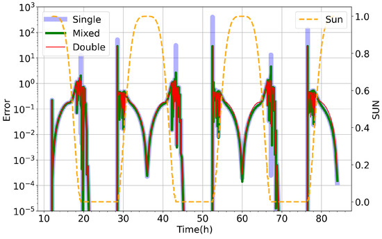
Figure 1.
Total species error () over time for small stratospheric model using Ros3 numerical solver for for out-of-the-box single precision (blue), double precision (red) and our implementation of mixed precision in KPP (green). We also show here the sunlight intensity (orange), which controls the onset, intensity and termination of atmospheric photochemistry.
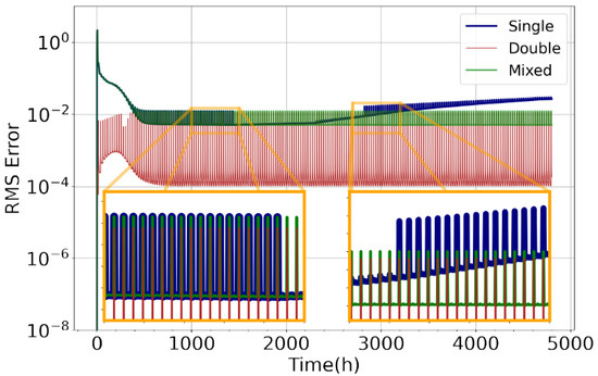
Figure 2.
RMS error compared to implicit solver with (Equation (8)) against time for CBM-IV chemistry model using Rodas3 numerical solver at by out-of-the-box single precision (blue), double precision KPP (red), and the new mixed-precision implementation (green).
4. Kinetic Pre-Processor Refactoring
We present code modifications for implementing an efficient mixed-precision KPP version in which all chemical species and reaction rates variables are stored in single precision. We eliminate the instances of high error in species concentrations and alleviate the extra required integration sub-steps, while maintaining numerical accuracy to five significant figures.
4.1. Data Structures
KPP generates source code that encompasses a number of data structures holding global variables that remain permanently in scope, such that the memory that they are occupying is not freed until the termination of the program. These include data structures of size equal to the total number of species (NSPEC) that hold the concentration of each species and are updated after every accepted integration sub-step, the number of reactions (NREACT) holding the photolysis and reaction rate constants, and the number of variable species (NVAR) holding the relative and absolute tolerance of each species. There is also a number of addresses for the simulation time and other physical variables, such as sunlight intensity and temperature.
In double precision, each data address requires 64 bits of memory to be stored, while single precision requires 32 bits of memory. The new implemented mixed-precision KPP converts all matrix elements and most of the variables that are globally defined in single precision. The rate constants are stored in single precision with a sufficient accuracy. Laboratory rate constants have large uncertainties as they are generally known within 1%. This corresponds to 2 significant digits, whereas single precision is represented with 7 significant digits. Following this approach, we have developed a new mixed-precision version that benefits from almost a factor of two reduction in memory but also overcomes the performance issues related to accuracy. In order to maintain accuracy and efficient time-step length control, the sunlight intensity and the variables that handle timing are maintained in double precision (Section 4.3).
4.2. Vectorisation
Moreover, we explicitly now exposed the KPP data structures to single instruction on multiple data (SIMD) vectorisation through the use of compiler intrinsic functions. Most modern CPUs can make use of this capability by relying on instructions sets such as Intel SSE and AVX, and while in many cases, a compiler will generate vector instructions automatically (auto-vectorisation), we were still able to obtain additional performance improvements (Section 5). All functions that handle linear algebra operations were modified with pre-processor directives to explicitly exploit vectorisation. We utilized __m128 registers that now pack four single-precision (float) variables instead of two in double precision. Specifically, the linear algebra routines in KPP that were overloaded with intrinsic implementations are: WCOPY, which copies a vector to another vector, WAXPY, which performs a scalar multiplication and a vector addition, WSCAL, which scales a vector by a zero, and WADD, which performs vector addition. These functions were used during the integration stage of the simulation, specifically in preparing the concentration, reaction constant and Jacobian matrices and computing each solver stage, the solution vector in each sub-step, and calculating the error. Finally, we additionally replaced all constant parameters from double to single precision to avoid type casting and replaced all math functions (other than the sunlight intensity calculation) that were optimized for double-precision arithmetic with their single-precision counterparts.
4.3. Time Step Length Control
As indicated in Section 3.5, error values are sensitive to the sun intensity values due to the onset of photochemistry. This is due to the calculation of the sun zenith angles at different machine precisions when the special math functions optimised for single precision are employed. Reduced precision results in inaccurate photolysis rate coefficients (also known as J-values) and rates for reactions triggered by the sun, causing great error deviations (as shown in Figure 1). A new mixed-precision version of the function that updates the sun intensity was implemented in place of the previous calculation, with accuracy equivalent to double-precision KPP.
Variables that handle timing and step size were also kept in double precision in order to ensure the numerical stability of the simulations and treat the growing error magnitude over time that manifests in single precision. This change leads to a marked improvement in the number of required integration sub-steps and a reduction in the cumulative integration output error, particularly important for longer simulations.
An additional optimisation is the introduction of adjustable δ in the evaluation of the time partial derivative of the function by finite differences (Equation (2)) depending on sunlight intensity. Sunlight intensity values that are required for the evaluation of the derivative are obtained at (where t is the current time of simulation). At sunset and sunrise, the critical values of T destabilize the simulations in single precision. To maintain numerical stability in these cases, is adjusted to use double precision for values of sunlight smaller than a pre-defined threshold. Thus, in place of Equation (3), we introduce:
where E is the machine epsilon at double precision, and is the machine epsilon of the working precision.
5. Performance Results
5.1. Accuracy and Precision
In this section, we present benchmarking results of the new mixed-precision implementation, and quantify the achieved benefits over single-precision KPP out-of-the-box.
Using the small stratospheric model on with the Ros3 solver, presented previously in Section 3.5, we are now able to completely remove the error peaks produced during sunrise and sunset, as shown in the total error over time for each precision (Figure 1).
Switching to the use of mixed precision drastically reduces the rejected sub-steps, consecutive rejections and accepted sub-steps with high error that require sub-step size reduction (Table 2). A great reduction in total sub-steps has been achieved compared to the out-of-the-box single-precision calculation while maintaining accuracy and significantly reducing memory demands compared to double precision.
Table 2.
Cumulative integration sub-steps with small mechanism at .
To evaluate model skill, we measured the RMS error over time for cbm4 on for the Ros3 stratospheric model on Rodas3 and Chapman on Ros2 for for the three versions of the code (presented in Figure 2). The new implementation has managed to produce stable and acceptable results for all models for the extended simulation times (200 days). Figure 3 demonstrates the relative difference for species concentrations in the stratosphere, comparing mixed precision with the equivalent double-precision simulation. In all cases, the relative difference of species is within 1.2%, while most of the species exhibit minimal differences. As depicted in Figure 3, for some species, such as CH3O, H and NO, larger relative differences are observed. These species appear in trace quantities, and their concentrations have reached the limit of precision. Since we are computing the ratio of these values and we are dividing with small numbers, there is a bigger relative difference. Although these concentrations are practically depleted, when comparing between the mixed and double precision, they differ. Furthermore, in certain cases, the simulation fails to complete in single precision due to continuous growing of the total error. In mixed precision, this issue is corrected, and all simulations reach completion with the total error bounded.
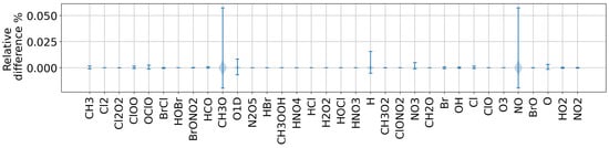
Figure 3.
Relative difference of species concentrations for the strato model with Ros4 solver for comparing the double-precision and the new mixed-precision implementation of KPP.
5.2. Vectorisation and Compiler Optimisations
To evaluate the achieved vector parallelisation performance when converted from the scalar implementation, all seven chemical mechanisms were benchmarked at different vectorisation operation levels: (i) with vectorisation disabled at compiling time; (ii) with automatic vectorisation by the compiler; and (iii) with SIMD vectorisation through compiler intrinsic functions.
The automatic vectoriser only achieves modest improvements due to an inability to resolve data dependencies, with a speedup not at any case greater than ∼5%. When Intel compiler intrinsic functions are used at the basic block- and loop-level, the achieved speed-up is between 10% and 25%. This is evident in Figure 4, which presents the speedup achieved by the compiler auto-vectorised code and by the explicitly vectorised code through intrinsics compared to the non-vectorised code for all seven mechanisms at relative tolerance for the Rodas4 solver in mixed precision.
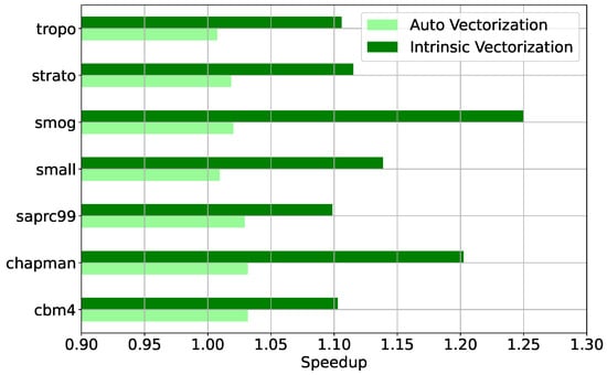
Figure 4.
Measured speed-up for the seven chemical mechanisms with mixed-precision Rodas4 at by automatic vectorisation (light green) and explicit vectorisation through the use of intrinsic functions (dark green) with respect to scalar code.
An additional gain in performance on the order of 30% was achieved, in part due to the reduced memory requirements, with compiler optimisations for fast performance, by enabling aggressive loop and memory-access optimizations, such as scalar replacement, loop unrolling and loop blocking to allow more efficient use of cache and additional data pre-fetching. By allowing reduced precision, we can utilise slightly less precise results than full IEEE division and perform floating calculations faster but with less accuracy, disabling floating-point exception semantics. Finally, we enabled inter-procedural optimization between files, code replication to eliminate branches, and static linking of libraries.
5.3. Performance at Scale
The experiments presented in the previous section were run in a box model configuration. In global CCM simulations, individual model grid cells are treated as box models following the operator split approach and are solved independently on each timestep of the global model. The scaling depends on the total number of grid cells, which is determined by the horizontal resolution, and on the number of vertical levels.
To demonstrate the performance gain by KPP in mixed precision for large-scale production simulations, we present projections with the EMAC global climate-chemistry model [32], with the Mainz organic mechanism (MOM) [37], a complex chemistry mechanism that includes 706 species in the gas phase and a total of 2130 reactions in order to capture organics in the atmosphere with explicit degradation of up to five carbon atoms and additional simplified chemistry for larger molecules.
Figure 5 shows the projected memory requirements for the MOM model, comparing single-, double- and mixed-precision KPP for seven horizontal resolutions commonly used [38] down to . The different resolutions quoted refer to the spherical harmonic wave number for a triangular truncation in a spectral representation of the prognostic fields, as used by ECMWF in the Integrated Forecasting System (IFS). Each spectral resolution corresponds to a Gaussian grid that is regular in longitude and almost regular in latitude, defined by the number of latitudinal increments between the Equator and the poles. For example, the N80 regular Gaussian grid is equivalent to the T159 spectral truncation with 80 gridpoints in the north and south latitudes. The number of vertical levels was set to either 31, as used in the ECMWF specification, with a top level at the 10 hPa pressure level, or to 90, which encompasses the stratosphere/middle atmosphere with the model top at 0.01 hPa.
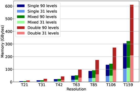
Figure 5.
Memory requirements in HPC simulations with KPP MOM chemical mechanism for different vertical configurations (31/90 levels) using single (blue/light blue), mixed (green/light green) and double (red/light red) precision for different spectral resolutions.
Mixed precision reduces the memory requirements for atmospheric chemical kinetics simulations by 47% compared to double precision. The total memory required is proportional to the number of model grid points, which is proportional to the product of the horizontal resolution in grid-point representation (lat × lon) and the number of -hybrid vertical levels.
A common bottleneck encountered in Earth system model simulations is failure to scale due to the high minimum memory per core requirement. This effectively limits the achieved speed-up. Mixed precision reduces memory requirements to about half of that for double precision, and model codes can scale to higher number of cores per RAM (intra-node) or with reduced RAM per node requirements. This is particularly important in the era of multi- to many-core CPUs as the cost per FLOP is dropping faster than the cost of memory.
Marked improvement can be expected in scaling efficiency and time-to-solution for all atmospherically relevant chemistry mechanisms of intermediate and advanced complexity across current and targeted spatial resolutions.
Beyond the atmospheric chemistry module (MECCA: Module Efficiently Calculating the Chemistry of the Atmosphere [28]), the EMAC model comprises two parts: the atmospheric general-circulation model, ECHAM (European Centre for Medium-Range Weather Forecasts Hamburg), and the modular framework, MESSy (Modular Earth Sub-model System), which links local physical processes to the base model. Benchmarking on the JUDGE cluster at the Jülich Supercomputing Centre (JSC) has shown that more than half and up to more than 85% of the total run time is required by KPP calculations [10].
The model was ported and benchmarked on a production-size machine at the MareNostrum supercomputer. Figure 6 presents a comparison of the experimentally verified total required runtime of the model measured on MareNostrum using the Mainz Inorganic Mechanism (MIM) at T42 resolution with 90 vertical levels in quasi chemistry-transport model (QCTM) configuration. QCTM allows for a quantification of chemical signals through suppression of feedback noise between chemistry and dynamics. The red hatched area indicates the improvement in runtime that can be achieved by the mixed precision KPP compared to the double precision code on top of the common dynamics and physics parameterisation components (ECHAM + MESSy). Though the scaling performance of the other components is severely limited due to the MPI communication pattern and load imbalance [10], EMAC can overall still scale and achieve reduced time-to-solution, beyond the double precision performance plateau, at higher core counts with mixed precision chemical kinetics.
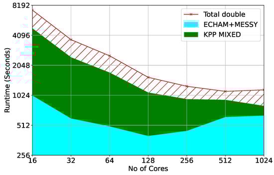
Figure 6.
Time-to-solution for EMAC model in QCTM configuration at T42L90 resolution: circulation dynamics ECHAM and physics MESSy (Cyan), and total required runtime in double precision (red). The red hatched area indicates the improvement in runtime that can be achieved by the mixed-precision KPP compared to the double-precision KPP.
Furthermore, mixed-precision KPP is expected to scale more efficiently than double precision at greater mechanism complexity. Theoretically, scaling should be perfect as grid cells are embarrassingly parallel. Figure 7 presents a comparison between the speed up of double precision and the projected speed up of mixed precision for the MOM mechanism at T42 resolution. As the problem of climate-chemistry modelling is memory-bound, the major challenge for large chemical mechanisms is the memory required per core, exacerbated by the trend of increasing core counts per CPU socket relative to the cost and availability of RAM per socket. This can lead to under-subscription of computational tasks to nodes in order to maintain the required minimum memory per core, burdening the inter- over the faster intra-node communication for nearest neighbour communication. As the new implementation can run on almost half the memory resources, it can provide additional benefits.
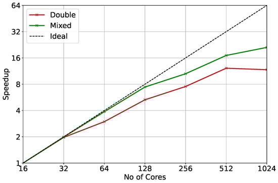
Figure 7.
Overall speed-up for double precision (red) and projection of improvement with mixed precision (green) for MOM mechanism at T42 resolution ().
Mixed precision allows simulations at resolutions that were previously inefficient. At the same time, the reduction in the required simulation time for any resolution enables simulations with higher complexity in chemical mechanisms. Finally, beyond the calculation of chemistry in the gas phase, our results can provide additional benefits in the use of KPP for the calculation of aqueous and heterogeneous chemistry in the condensed phase (aerosol) components of Earth system models.
The new mixed-precision implementation of KPP has been ported onto GPU accelerators using the MEDINA [39] code parser to generate CUDA kernels. Previous studies [11,40] showed a 1.75× speed-up over the non-accelerated application using the three-stage Rosenbrock solver in double precision. Running the MEDINA unit tests with our reduced precision implementation showed a promising additional performance speed-up by a factor of two for all Rosenbrock and Rodas solvers using the MIM chemistry mechanism. The median relative difference of concentrations was found to be less than 5% when compared to the double non-accelerated version throughout, only limited by the single-precision representation for depleted species with concentrations equivalent to zero.
6. Conclusions
The aim of this work is to develop an efficient implementation of an atmospheric chemical kinetics solver template in mixed precision, with the bulk of the variable addresses stored in single precision [12] to benefit from almost halving of the required memory for computations. Variables critical for the accuracy of the simulations are kept in double precision in order to maintain numerical stability.
Reduced-precision arithmetic is shown to require only a marginally increased (∼3%) number of integration sub-steps compared to out-of-the-box double precision while reducing the sub-steps required for pure single-precision calculations by ×1.5-fold on average and up to ×3-fold.
For memory-intensive HPC simulations, where performance is limited by available cache and random access memory, as is the case for atmospheric chemical kinetics, refactoring from double to single precision can offer a speed-up by a factor of up to two [2]. We note that refactoring software to run on single rather than double precision may not necessarily increase expected peak flop rate on standard consumer CPUs built on intrinsic 64-bit architectures.
The achieved performance is additionally improved by explicit vectorisation through intrinsic functions. Depending on the level of vectorisation of the code, the processing unit can perform multiple floating point operations simultaneously and speed up the overall simulation by an additional factor of up to two. This factor is highly dependent on the system vector unit size and the ability of the compiler to expose the vectorisation automatically. In the experiments described in this paper, the achieved additional performance speed-up on top of the heuristic auto-vectoriser at maximum optimisation level for KPP is in the range of ∼10% to 25%, dependent on the chemical mechanism and numerical solver.
Another primary concern is the accuracy level of these simulations. The goal is to minimize to the extent possible compromises in accuracy when refactoring from double to mixed precision. As evidenced by the metrics in Section 5, the new mixed-precision version of KPP can replicate results of the double-precision code generated by KPP within a maximum relative difference of ∼1%, which was much lower in most cases.
The new implementation is able to also maintain the error stability in simulations, countering the growth of error over time in the out-of-the-box single implementation of KPP. The mixed-precision simulations are generally stable in terms of RMS error, as is the case for double precision, while keeping the error at tolerable levels compared to double-precision RMSE over long integration periods.
The reduction in required memory for the calculation of the atmospheric chemistry component in Earth system models can amplify the performance boost shown by porting the code to GPU architectures [11,40], where the memory overflow issues are the main limiting factor [39]. Finally, the reduction in memory requirements can serve to future-proof the numerous geoscientific models that rely on KPP against new and novel hardware architectures towards exploiting the potential of the emerging Exascale platforms.
Our results suggest that reduced-precision chemical kinetics can allow a significant reduction in computational requirements and/or increase of complexity in climate-chemistry simulations.
Author Contributions
K.S.: Investigation, Software, Visualization, Writing—original draft. T.C.: Funding acquisition, Methodology, Supervision, Writing—review & editing. All authors have read and agreed to the published version of the manuscript.
Funding
This research article has been produced within the framework of the projects EMME-CARE, which has received funding from the European Union’s Horizon 2020 Research and Innovation Programme (under grant agreement no. 856612) and the Cyprus Government, and NI4OS-Europe funded by the European Commission under the Horizon 2020 European research infrastructures grant agreement no. 857645.
Acknowledgments
The authors wish to thank Rolf Sander (Air Chemistry Department, Max Planck Institute for Chemistry) for the insightful comments and suggestions on how to improve the manuscript.
Conflicts of Interest
The authors declare no conflict of interest.
References
- Masson-Delmotte, V.; Zhai, P.; Pirani, A.; Connors, S.L.; Péan, C.; Berger, S.; Caud, N.; Chen, Y.; Goldfarb, L.; Gomis, M.I.; et al. (Eds.) Climate Change 2021: The Physical Science Basis. Contribution of Working Group I to the Sixth Assessment Report of the Intergovernmental Panel on Climate Change; Cambridge University Press: Cambridge, UK, 2021; in press. [Google Scholar]
- Düben, D.P.; Palmer, T.N. Benchmark tests for numerical weather forecasts on inexact hardware. Mon. Weather. Rev. 2014, 142, 3809–3829. [Google Scholar] [CrossRef]
- Nakano, M.; Yashiro, H.; Kodama, C.; Tomita, H. Single precision in the dynamical core of a nonhydrostatic global atmospheric model: Evaluation using a baroclinic wave test case. Mon. Weather. Rev. 2018, 146, 409–416. [Google Scholar] [CrossRef]
- Wedi, N.P. Increasing horizontal resolution in numerical weather prediction and climate simulations: Illusion or panacea? Philos. Trans. R. Soc. Math. Phys. Eng. Sci. 2014, 372, 20130289. [Google Scholar] [CrossRef] [PubMed]
- Masters, J. IBM Introducing the World’s Highest-Resolution Global Weather Forecasting Model. Weather Underground. Available online: https://www.wunderground.com/cat6/IBM-Introducing-Worlds-Highest-Resolution-Global-Weather-Forecasting-Model (accessed on 8 January 2019).
- Shapiro, M.; Shukla, J.; Brunet, G.; Nobre, C.; Béland, M.; Dole, R.; Wallace, J.M. An earth-system prediction initiative for the twenty-first century. Bull. Am. Meteorol. Soc. 2010, 91, 1377–1388. [Google Scholar] [CrossRef][Green Version]
- Shukla, J.; Palmer, T.; Hagedorn, R.; Hoskins, B.; Kinter, J.; Marotzke, J.; Miller, M.; Slingo, J. Toward a new generation of world climate research and computing facilities. Bull. Am. Meteorol. Soc. 2010, 91, 1407–1412. [Google Scholar] [CrossRef]
- Yashiro, H.; Terasaki, K.; Kawai, Y.; Kudo, S.; Miyoshi, T.; Imamura, T.; Tomita, H. A 1024-member ensemble data assimilation with 3.5-km mesh global weather simulations. In Proceedings of the SC20: International Conference for High Performance Computing, Networking, Storage and Analysis, Atlanta, GA, USA, 9–19 November 2020; IEEE: Piscataway, NJ, USA, 2020. [Google Scholar]
- Zhang, H.; Linford, J.C.; Sandu, A.; Sander, R. Chemical mechanism solvers in air quality models. Atmosphere 2011, 2, 510–532. [Google Scholar] [CrossRef]
- Christou, M.; Christoudias, T.; Morillo, J.; Alvarez, D.; Merx, H. Earth system modelling on system-level heterogeneous architectures: EMAC (version 2.42) on the Dynamical Exascale Entry Platform (DEEP). Geosci. Model Dev. 2016, 9, 3483–3491. [Google Scholar] [CrossRef]
- Alvanos, M.; Christoudias, T. Accelerating Atmospheric Chemical Kinetics for Climate Simulations. IEEE Trans. Parallel Distrib. Syst. 2019, 30, 2396–2407. [Google Scholar] [CrossRef]
- IEEE Std 754–2008; IEEE Standard for Floating-Point Arithmetic. IEEE: Piscataway, NJ, USA, 2008; pp. 1–70. [CrossRef]
- Düben, P.D.; McNamara, H.; Palmer, T.N. The use of imprecise processing to improve accuracy in weather & climate pre-diction. J. Comput. Phys. 2014, 271, 2–18. [Google Scholar] [CrossRef]
- Düben, P.D.; Russell, F.P.; Niu, X.; Luk, W.; Palmer, T.N. On the use of programmable hardware and reduced numerical precision in earth-system modeling. J. Adv. Model. Earth Syst. 2015, 7, 1393–1408. [Google Scholar] [CrossRef]
- Düben, P.; Diamantakis, M.; Lang, S.; Saarinen, S.; Sandu, I.; Wedi, N. Tomas WilhelmssonProgress in using single precision in the IFS. ECMWF Newsl. 2018, 157, 26–31. Available online: https://www.ecmwf.int/en/elibrary/18705-newsletter-no-157-autumn-2018 (accessed on 5 April 2022).
- Palem, K.V. Energy aware algorithm design via probabilistic computing: From algorithms and models to Moore’s law and novel (semiconductor) devices. In Proceedings of the 2003 International Conference on Compilers, Architecture, and Synthesis for Embedded Systems, San Jose, CA, USA, 30 October–1 November 2003; IEEE: Piscataway, NJ, USA; pp. 113–116. [Google Scholar] [CrossRef]
- Palem, K.V. Energy aware computing through probabilistic switching: A study of limits. IEEE Trans. Comput. 2005, 54, 1123–1137. [Google Scholar] [CrossRef]
- Palem, K.V.; Lingamneni, A. Ten years of building broken chips: The physics and engineering of inexact computing. ACM Trans. Embedded Comput. Syst. 2013, 12, 87. [Google Scholar] [CrossRef]
- Sartori, J.; Sloan, J.; Kumar, R. Stochastic computing: Embracing errors in architecture and design of processors and applications. In Proceedings of the 2011 International Conference on Compilers, Architecture, and Synthesis for Embedded Systems, Taipei, Taiwan, 9–14 October 2011; IEEE: Piscataway, NJ, USA; pp. 135–144. [Google Scholar]
- Palem, K.V. Inexactness and a future of computing. Philos. Trans. R. Soc. 2014, 372A, 2018. [Google Scholar] [CrossRef] [PubMed][Green Version]
- Madec, G. NEMO Ocean Engine, Note du Pole de Modelisatio. 2008, pp. 1288–1619. Available online: https://www.nemo-ocean.eu/wp-content/uploads/Doc_OPA8.1.pdf (accessed on 1 July 2019).
- Dawson, A.; Düben, P.D. Rpe v5: An emulator for reduced floating-point precision in large numerical simulations. Geosci. Model Dev. 2017, 10, 2221–2230. [Google Scholar] [CrossRef]
- Tintó Prims, O.; Acosta, M.C.; Moore, A.M.; Castrillo, M.; Serradell, K.; Cortés, A.; Doblas-Reyes, F.J. How to use mixed precision in ocean models: Exploring a potential reduction of numerical precision in NEMO 4.0 and ROMS 3.6. Geosci. Model Dev. 2019, 12, 3135–3148. [Google Scholar] [CrossRef]
- Moore, A.; Arango, H.; Broquet, G.; SPowell, B.; Weaver, A.; Zavala-Garay, J. The Regional Ocean Modeling System (ROMS) 4-dimensional variational data assimilation systems Part I—System overview and formulation. Prog. Oceanogr. 2011, 91, 34–49. [Google Scholar] [CrossRef]
- Colin, A.J. CHEMSODE: A stiff ODE solver for the equations of chemical kinetics. Comput. Phys. Commun. 1996, 97, 304–314. [Google Scholar]
- Damian, V.; Sandu, A.; Damian, M.; Potra, F.; Carmichael, G.R. The kinetic preprocessor KPP-a software environment for solving chemical kinetics. Comput. Chem. Eng. 2002, 26, 1567–1579. [Google Scholar] [CrossRef]
- Adrian, S.; Sander, R. Simulating chemical systems in Fortran90 and Matlab with the Kinetic PreProcessor KPP-2.1. Atmos. Chem. Phys. 2006, 6, 187–195. [Google Scholar]
- Sander, R.; Baumgaertner, A.; Gromov, S.; Harder, H.; Jöckel, P.; Kerkweg, A.; Kubistin, D.; Regelin, E.; Riede, H.; Sandu, A.; et al. The atmospheric chemistry box model CAABA/MECCA-3.0. Geosci. Model Dev. 2011, 4, 373–380. [Google Scholar] [CrossRef]
- Peckham, S.E. WRF/Chem Version 3.3 User’s Guide; National Center for Atmospheric Research (NCAR): Boulder, CO, USA, 2012. [Google Scholar]
- Lu, S.; Jacob, D.J.; Santillana, M.; Wang, X. An adaptive method for speeding up the numerical integration of chemical mechanisms in atmospheric chemistry models: Application to GEOS-Chem version 12.0.0. Geosci. Model Dev. 2020, 13, 2475–2486. [Google Scholar]
- Martin, R.V.; Eastham, S.D.; Bindle, L.; Lundgren, E.W.; Clune, T.L.; Keller, C.A.; Downs, W.; Zhang, D.; Lucchesi, R.A.; Sulprizio, M.P.; et al. Improved Advection, Resolution, Performance, and Community Access in the New Generation (Version 13) of the High Performance GEOS-Chem Global Atmospheric Chemistry Model (GCHP). Geosci. Model Dev. Discuss. 2022, 1–30, in press. [Google Scholar]
- Jöckel, P.; Kerkweg, A.; Pozzer, A.; Sander, R.E.; Tost, H.; Riede, H.; Baumgaertner, A.; Gromov, S.; Kern, B. Development cycle2 of the Modular Earth Submodel System (MESSy2). Geosci. Model Dev. 2010, 3, 717–752. [Google Scholar] [CrossRef]
- Gery, M.W.; Whitten, G.Z.; Killus, J.P.; Dodge, M.C. A photochemical kinetics mechanism for urban and regional scale computer modeling. J. Geophys. Res. Atmos. 1989, 94, 12925–12956. [Google Scholar] [CrossRef]
- Cao, L.; Li, S.; Yi, Z.; Gao, M. Simplification of Carbon Bond Mechanism IV (CBM-IV) under Different Initial Conditions by Using Concentration Sensitivity Analysis. Molecules 2019, 24, 2463. [Google Scholar] [CrossRef] [PubMed]
- Carter, W.P.L. Documentation of the SAPRC-99 chemical mechanism for VOC reactivity assessment. Contract 2000, 92, 95–308. [Google Scholar]
- Ernst, H.; Wanner, G. Stiff differential equations solved by Radau methods. J. Comput. Appl. Math. 1999, 111, 93–111. [Google Scholar]
- Pozzer, A.; Reifenberg, S.F.; Kumar, V.; Franco, B.; Kohl, M.; Taraborrelli, D.; Gromov, S.; Ehrhart, S.; Jöckel, P.; Sander, R.; et al. Simulation of organics in the atmosphere: Evaluation of EMACv2. 54 with the Mainz Organic Mechanism (MOM) coupled to the ORACLE (v1. 0) submodel. Geosci. Model Dev. 2022, 15, 2673–2710. Available online: https://gmd.copernicus.org/articles/15/2673/2022/ (accessed on 1 April 2022). [CrossRef]
- Roeckner, E.; Bäuml, G.; Bonaventura, L.; Brokopf, R.; Esch, M.; Giorgetta, M.; Hagemann, S.; Kirchner, I.; Kornblueh, L.; Manzini, E.; et al. The Atmospheric General Circulation Model ECHAM 5. PART I: Model Description; Max Planck Society: Munich, Germany, 2003. [Google Scholar]
- Christoudias, T.; Kirfel, T.; Kerkweg, A.; Taraborrelli, D.; Moulard, G.; Raffin, E.; Azizi, V.; Oord, G.; Werkhoven, B. GPU Optimizations for Atmospheric Chemical Kinetics. In Proceedings of the HPC Asia 2021: The International Conference on High Performance Computing in Asia-Pacific Region, Virtual, 20–21 January 2021; pp. 136–138. [Google Scholar]
- Alvanos, M.; Christoudias, T. GPU-accelerated atmospheric chemical kinetics in the ECHAM/MESSy (EMAC) Earth system model (version 2.52). Geosci. Model Dev. 2017, 10, 3679–3693. [Google Scholar] [CrossRef]


Publisher’s Note: MDPI stays neutral with regard to jurisdictional claims in published maps and institutional affiliations. |
© 2022 by the authors. Licensee MDPI, Basel, Switzerland. This article is an open access article distributed under the terms and conditions of the Creative Commons Attribution (CC BY) license (https://creativecommons.org/licenses/by/4.0/).