Chemical Composition and Source Apportionment of Winter Fog in Amritsar: An Urban City of North-Western India

Abstract

Winter fog is a complex issue affecting human health and is responsible for higher numbers of traffic accidents in North India, which is further aggravated due to atmospheric pollutants. An indigenous glass-plate fog collector was used to collect fog water from December 2020 to February 2021. Thirty samples of fog water were collected from the rooftop of an academic building at Guru Nanak Dev University, Amritsar, in order to study the chemistry of fog water. The studied parameters were pH, electrical conductivity (EC), sodium (Na⁺), calcium (Ca²⁺), magnesium (Mg²⁺), potassium (K⁺) sulphate (SO₄²⁻), nitrate (NO₃⁻), chloride (Cl⁻), aluminum (Al), lead (Pb) and zinc (Zn). The average values were as follows: pH (4.6–7.5), EC (135 µS/cm), SO₄²⁻ (77.5 ppm), Cl⁻ (9.9 ppm), NO₃⁻ (9.3 ppm), Ca²⁺ (8.1 ppm), Mg²⁺ (2.0 ppm), K⁺ (2.0 ppm), Na⁺ (1.6 ppm), Zn (218 ppb), Al (60.8 ppb) and Pb (8.8 ppb). Cation–anion balance was used to assess the data’s reliability. The enrichment factor (EF) was utilized to distinguish between crustal and anthropogenic sources. SO₄²⁻, NO₃⁻, Cl⁻ and K⁺ originated from anthropogenic sources, whereas Mg²⁺ and Na⁺ came from crustal sources. The molar ratio of sulphate to nitrate was 10.6, which indicates a greater contribution from the combustion of fossil fuels and stack emissions. Ionic species were subjected to principal component analysis (PCA) as a dimensionality reduction approach and to group species with comparable behavior. Three principal components (PC) that together accounted for 77.5 percent of the total variance were identified by PCA. Backward trajectory analysis of air masses was performed to determine their origin, and two major clusters explained 89 percent of the contribution of air masses, primarily from the north-east and north directions. To gain a comprehensive understanding of fog water, a global perspective on pH, EC and ionic species is considered.

1. Introduction

Fog and haze are correlated with relative humidity (RH), PM_2.5 levels, wind speed and the height of the planetary boundary layer [1]. Aerosol particles can build up in the boundary layer under unfavorable dispersion conditions, resulting in air pollution, which has a negative impact on human health and atmospheric visibility. Fog is a meteorological phenomenon that occurs when a cloud of small water droplets near the ground surface becomes dense enough to reduce horizontal visibility to less than 1 km [2]. Because they wash out various aerosol particles as they fall to the Earth’s surface, fog and rain can both act as natural cleaners of the lower atmosphere [3]. Due to increased air pollution from various sources, the frequency of fog occurrence dominates in urban areas [2,4,5] with lower temperatures and saturation; urbanization delays the formation of low-level fog by 3 h and accelerates its dissipation by 1.5 h [6]. During the winter months of December and January, dense fog is observed over the Indo-Gangetic Plains (IGP) [7]. These severe fog events have a wide-ranging impact, including on aviation and road transportation, resulting in an increasing number of traffic accidents [8]. Low temperatures, a calm atmosphere and a boundary layer height of 500 m to 800 m increase the concentration of aerosol particles in the lower atmosphere during the winter season [9]. Furthermore, aerosols contribute to fog formation by altering microphysical properties, such as increasing the liquid water content and droplet concentration and decreasing the droplet effective radius [3,6]. Thus, characterizing the acidity of fog and rainwater is critical for gaining a better understanding of acidic deposition inputs at high elevations [10]. The chemistry of fog water varies greatly depending on the location. The chemical composition of fog water has been highlighted by various researchers in various parts of the world [1,10,11,12,13,14,15,16].

The multi-dimensional characterization of fog water is critical for determining the possible sources of various ions and metals estimated in fog water samples. The determination of trace metals is important due to their toxicity to the environment. Previous studies on trace metal estimation include Wang et al. [10], Li et al. [11], Bianco et al. [12] and Liu et al. [17]. According to Bianco et al. [12], the most abundant elements are Zn and Mg. Few previous studies on aerosol mass loading in Amritsar during the winter months have been conducted [18,19,20]. Previous source apportionment studies have been carried out using a variety of techniques, such as enrichment factor and principal component analysis [10,21,22]. There is a vast amount of research that focuses on the characterization of fog, but studies of the sources and air masses are scarce. In-depth investigations of the composition of urban fog and its many sources will be more helpful in designing management methods in the city, taking into account the potential effects of dense fog over the area.

Over the past few decades, research on the chemistry of fog water has grown in importance. In India, the study of fog composition is not sufficiently conducted compared to the international assessment of fog research. As a result, the goal of the current study is to evaluate the composition of winter fog and the contributing possible sources by incorporating different source identification techniques. Additionally, we examine how global and regional air mass movements affect the chemistry of fog water.

2. Materials and Methods

2.1. Site Description

Amritsar is a city in the north-western Indian state of Punjab, 30 kilometers from the Pakistani border, with geographical coordinates of 31.3429 to 31.4227° N and 74.4748 to 74.5558° E (Figure 1) and four seasons: winter (December to March), summer (April to June), rainy (July to August) and post-monsoon (September to November). Amritsar has a population of over one million inhabitants and a population density of 8100 persons per square kilometer. It also has major industrial clusters in the east, west and south of the city. There are nearly 20,200 industrial units registered with the Punjab Pollution Control Board, which include textiles, dyes, pharmaceuticals and engineering, among other fields.

2.2. Sample Collection

Fog samples were collected using an inclined glass (50 cm × 50 cm) installed on the rooftop of Guru Nanak Dev University, Amritsar, and the line diagram of fog collection depicted in our previous publication [23]. The sampling occurred between 29 December 2020 and 20 February 2021. In a pre-washed glass container, samples were collected during night hours (6 a.m. to 6 p.m.), and any sample volume less than 50 mL was discarded as non-representative. The pH and electrical conductivity (EC) of all collected fog water were immediately determined using a pre-calibrated three-decimal digital pH meter (Labtronics, LT-501) and EC meter (Labtronics, LT-51). All the samples were filtered with a 0.45 μm cellulose nitrate membrane filter and transferred to clean PET plastic bottles. The samples were stored at 4 °C in a refrigerator for further analysis.

2.3. Ionic Composition of Fog Samples and Anion–Cation Balance Check

Sodium (Na⁺), potassium (K⁺), calcium (Ca⁺), magnesium (Mg²⁺), aluminum (Al), lead (Pb) and zinc (Zn) were measured using a sophisticated analytical microwave plasma-atomic emission spectrophotometer (Agilent, 4200 MP-AES). SO₄²⁻, NO₃⁻ and Cl⁺ concentrations were determined using the turbidimetric method (4500-SO₄²⁻ E), the UV–spectrophotometric screening method (4500-NO₃⁻ B) and the argentometric titration method (4500-Cl⁻ B), as described in Standard Methods for the Examination of Water and Wastewater, respectively [24]. The data quality was checked using the anion–cation balance as per Equation (1). A percentage difference up to 20% is considered good, but in our case, the sum of cations was significantly lower than the sum of anions due to not testing NH₄⁺ ions.

$$\% difference=100\ast \frac{\sum Anions-\sum Cations}{\sum Anions+\sum Cations}$$

(1)

2.4. Neutralization Factor (NF)

The neutralization factor measures the effectiveness of base cations (Ca²⁺, Mg²⁺, K⁺ and NH₄⁺) in neutralizing acid anions such as sulphate and nitrate [22,25,26,27,28]. The empirical Equation (2) was used to determine the role of cations in controlling the acidity of atmospheric deposition:

$$Neutralizing factor \left(NF\right)=X/\left(SO4+NO3\right)$$

(2)

where ‘X’ is the corresponding cation for which the neutralizing factor is to be calculated. All the values are in mg/L.

2.5. Enrichment Factor (EF)

The enrichment factor (EF) has been widely used to study the contributions of sea salt and crustal major ions in fog, rain and dew waters [10,22,29,30,31]. In general, Na⁺ and Ca²⁺ are used as sea and crust reference elements, respectively, and are widely used background tracers for marine and crustal sources. The enrichment factor in fog in relation to concentrations in the sea and crust was calculated using Equations (3) and (4). An enrichment factor of less than one (EF < 1) indicates that there is no enrichment from sources other than the sea and crust, whereas a value greater than one (EF > 1) indicates enrichment of specific species from non-sea sources [21,27,30,32].

$$Enrichment factor \left(sea\right)=\frac{\left(\frac{X}{Na}\right)Sample}{\left(\frac{X}{Na}\right)Sea}$$

(3)

where ‘X’ is the ion of interest, i.e., Ca²⁺, Mg²⁺, K⁺, SO₄⁻, NO₃⁻ and Cl⁻.

$$Enrichment factor \left(crust\right)=\frac{\left(\frac{X}{Ca}\right)Sample}{\left(\frac{X}{Ca}\right)Crust}$$

(4)

where ‘X’ is the ion of interest, i.e., Na⁺, Mg²⁺, K⁺, SO₄²⁻, NO₃⁻ and Cl⁻.

2.6. Principal Component Analysis

Principal component analysis (PCA) is a technique for reducing multidimensionality. In a group of independent variables, major principal components (PCs) are aligned, and similarly behaving variables are grouped. Version 23 of the Statistical Package for Social Sciences (SPSS). PCA was used in this study, with ten variables (SO₄²⁻, NO₃⁻, Cl⁻, Na⁺, K⁺, Ca²⁺, Mg²⁺, Al, Pb and Zn). PCs were chosen by combining a scree plot and eigenvalues greater than one to limit the PCs to explain 77.2 percent of the variance. Finally, varimax-rotated principal component analysis was used, with factor loading greater than 0.6. A 3-dimensional cube was used to visualize the factor loading plot.

2.7. Air Mass Back Trajectories

The back trajectory of air masses was used to determine their origin and relative contribution. The National Oceanic and Atmospheric Administration (NOAA) Air Resource Laboratory’s Hybrid Single-Particle Lagrangian Integrated Transport (HYSPLIT) model was studied at 500 m above ground level on various sampling days. For vertical profiling, all backward trajectories were calculated using the National Centers for Environmental Prediction (NCEP) Global Data Assimilation System (GDAS).

3. Results and Discussion

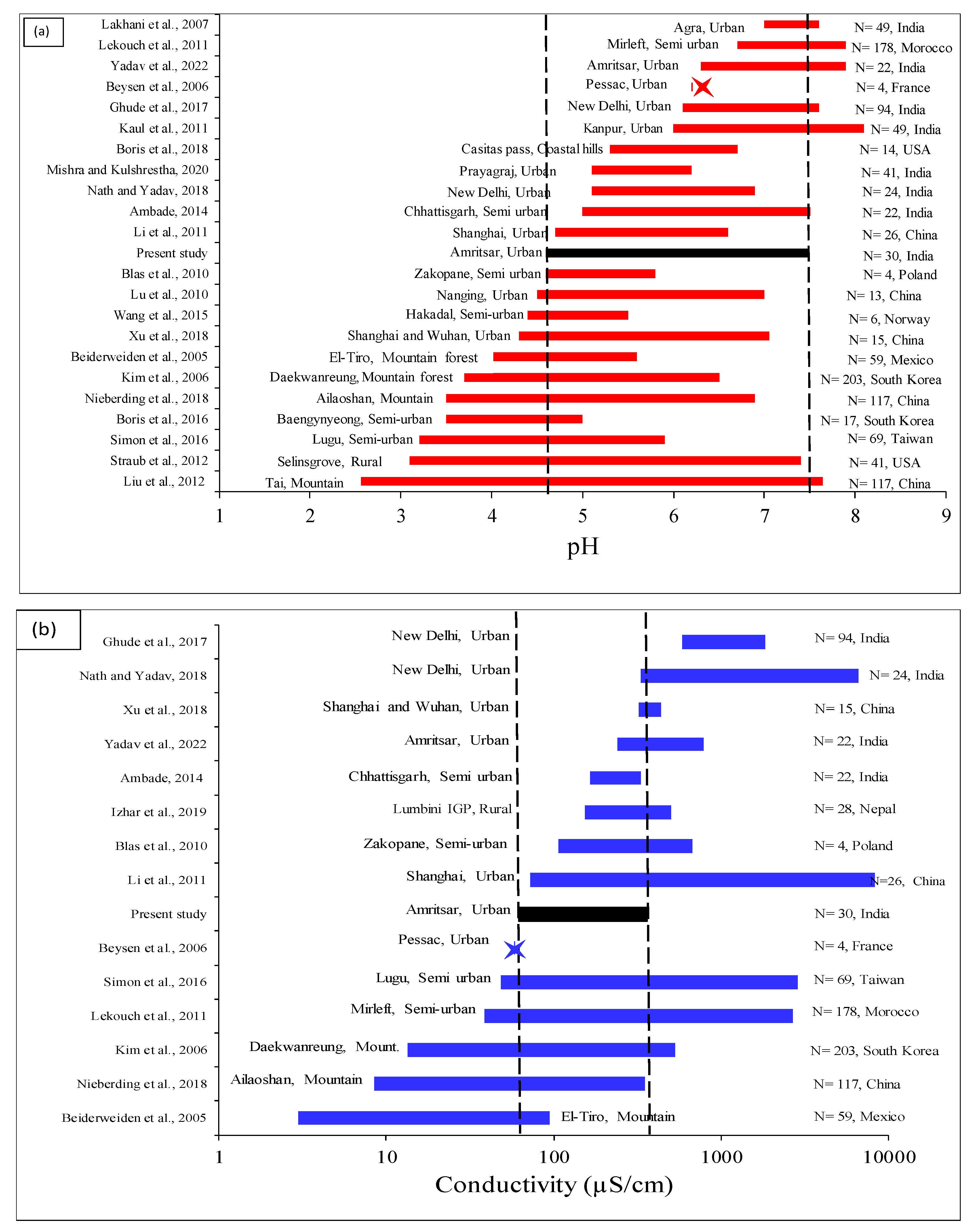
The fog water composition reveals the types of contaminants. The raw data are presented in Table S1, and an ionic balance check revealed a 42 percent difference, which is more than the 20 percent permitted limit. The absence of NH₄⁺ ion testing is the cause of the low cation sum.

3.1. pH

The pH of the fog water was measured, and the reported values ranged from 4.6 to 7.5. In the current study, 60 percent of the samples (n = 18) had a pH range of 6.0–6.8 and 20 percent of the samples (n = 6) had a pH range of 6.8–7.5. A minimum pH of 4.6 was obtained on two consecutive days (7 January 2021 and 12 January 2021), which could be attributed to high levels of SO₂ and NO₂ in the atmosphere. In contrast to the pH reported by Yadav et al. [23], a study conducted in Amritsar reported a pH range of 6.3 to 7.9. Although present fog water has a mean pH of 6.4, a pH less than 5.6 is considered acid rain [27,29,30]. To investigate the pH of fog water, a comprehensive literature review was conducted. Approximately fifteen international studies were conducted in countries such as China (five studies), South Korea (two studies) and the United States (two studies), with one study each from France, Morocco, Poland, Norway, Taiwan and Mexico. The minimum pH range was obtained for Tai Mountain, China, and the reason for this low value was attributed to the large amount of H₂SO₄ produced during aqueous-phase SO₂ oxidation [17], with the results shown in Figure 2a. Global perspective of (a) pH and (b) conductivity in fog water studies are shown in Figure 2 [8,17,23,26,33,34,35,36,37,38,39,40,41,42,43,44,45,46,47,48,49,50].

3.2. Electrical Conductivity

Electrical conductivity (EC) was found to be in the (62–365) μS/cm range, with an average value of 135 μS/cm. On January 1, 2021, the highest conductivity value of 365 μS/cm was recorded. Approximately 80% of the collected samples had conductivity in the (62–138) μS/cm range, which is comparable to other studies (Figure 2b). Shanghai had the highest EC values of 2050 μS/cm [41], which was due to the higher overall ionic concentration of fog water. In contrast, Yadav et al. [23] reported an average EC value of 450 μS/cm, with a range of 240 to 790 μS/cm, over Amritsar city during the winter of 2017 and 2018. The current study obtained lower EC values than previous studies.

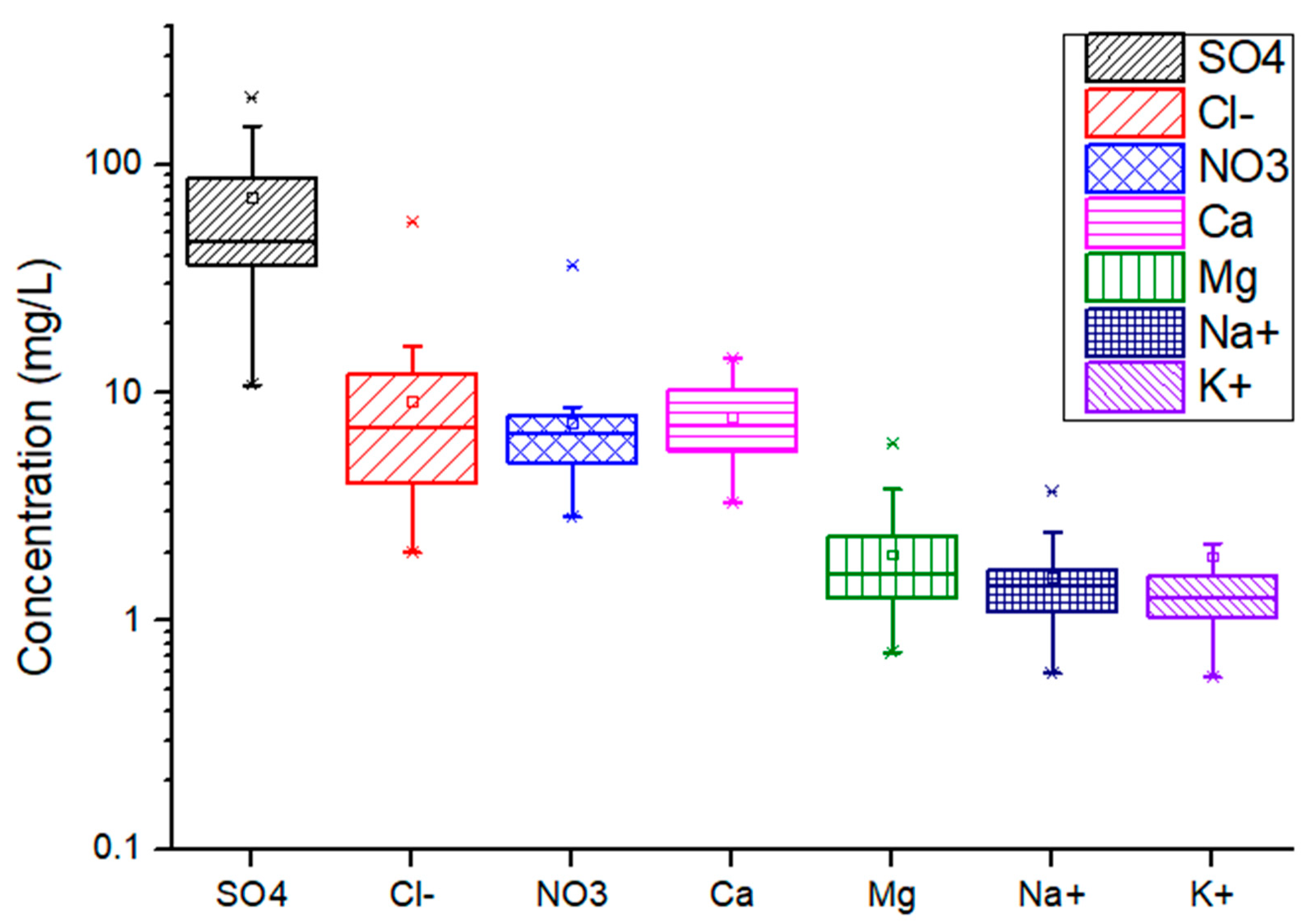
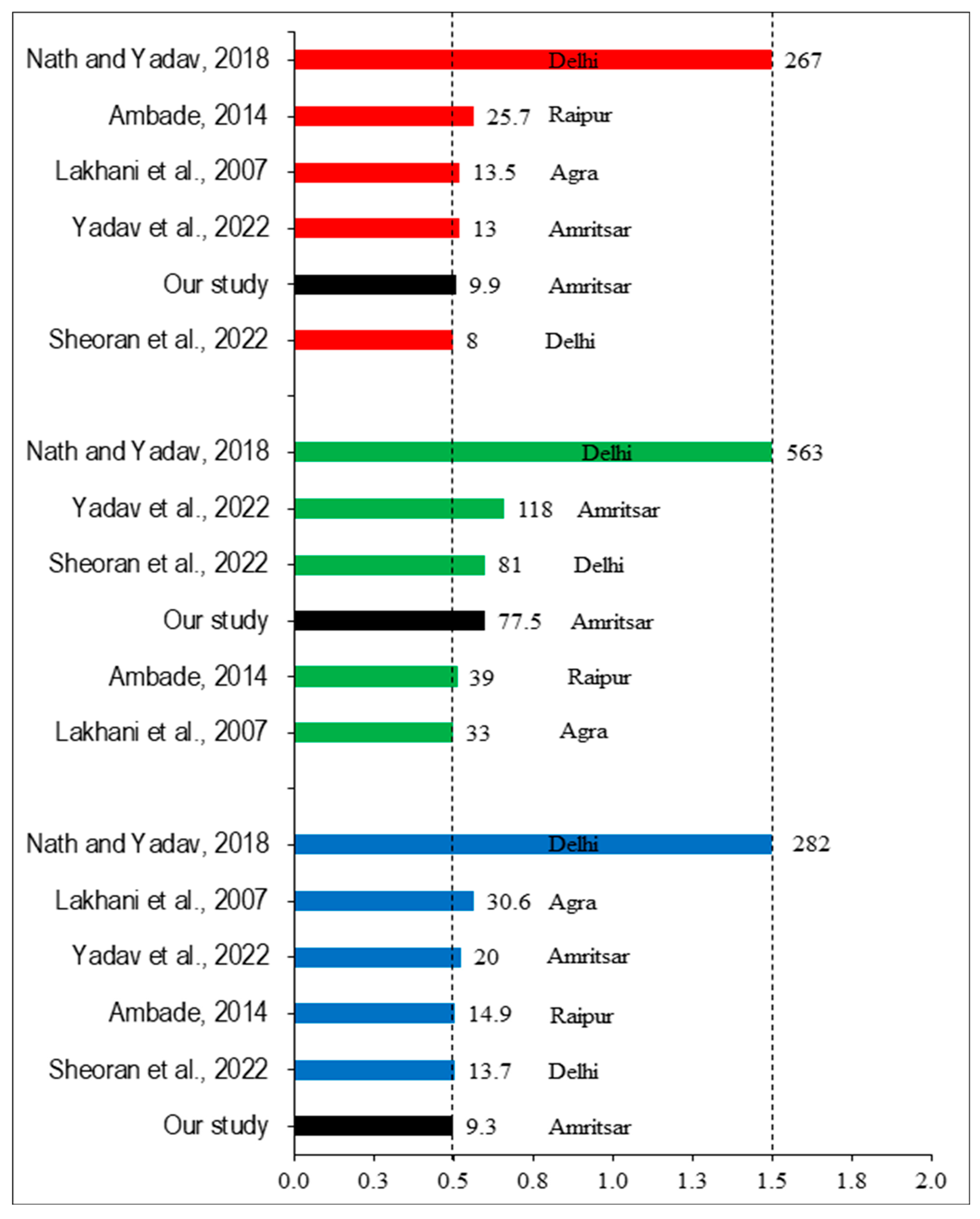
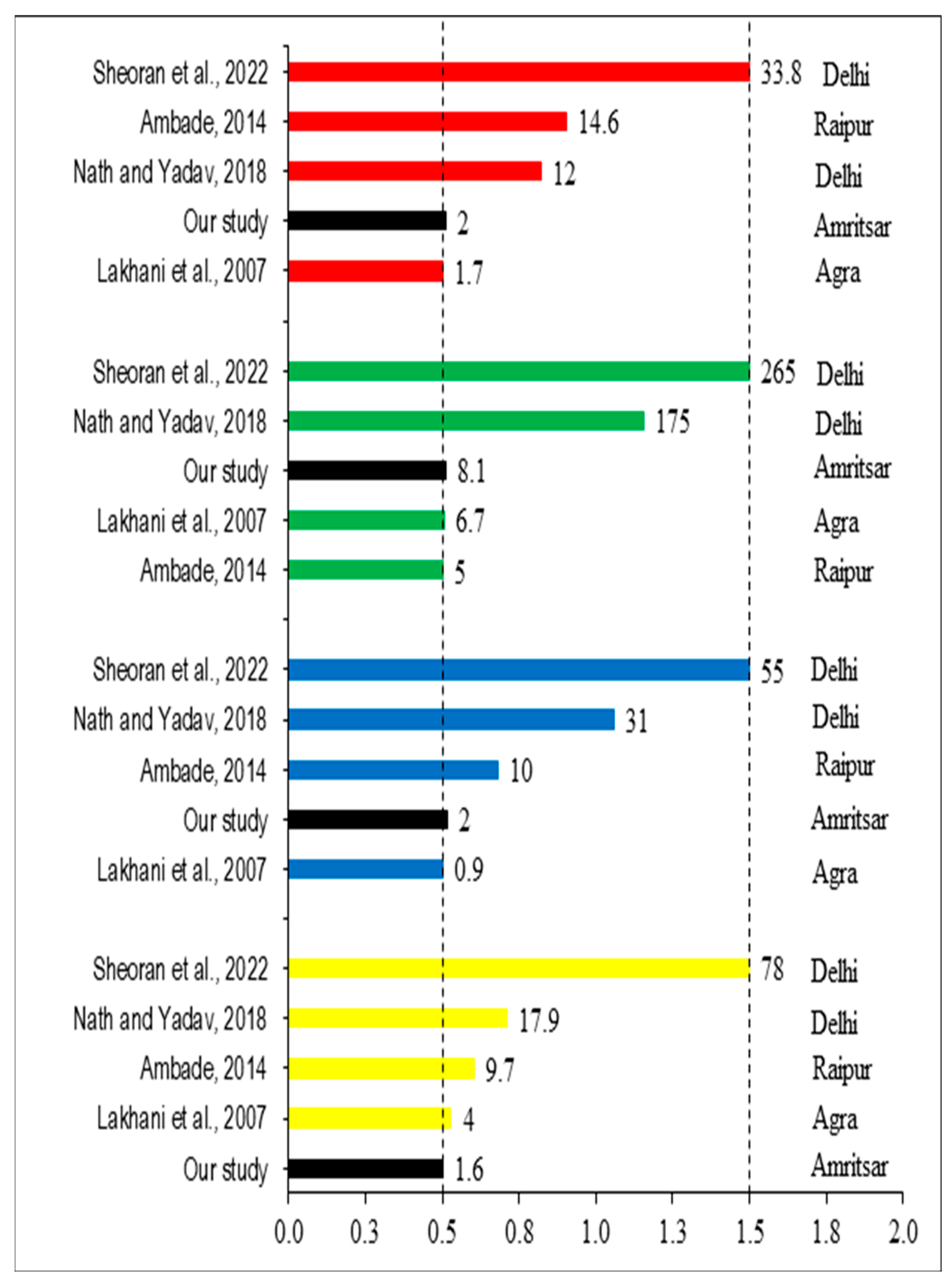
3.3. Ionic Composition and Trace Metals in Fog Water

The ionic composition indirectly reveals atmospheric pollutants as well as dominant species. The average values were SO₄²⁻ (77.5 ppm), Cl⁻ (9.9 ppm), NO₃⁻ (9.3 ppm), Ca²⁺ (8.1 ppm), Mg²⁺ (2.0 ppm), K⁺ (2.0 ppm), Na⁺ (1.6 ppm), Zn (218 ppb), Al (60.8 ppb) and Pb (8.8 ppb). As shown in Figure 3, the dominant species were SO₄²⁻ > Cl⁻ > N₃⁻ > Ca²⁺ > Mg²⁺ > Na⁺ > K⁺. One study reported sulphate > chloride > nitrate dominance [40], whereas other Indian studies reported sulphate > nitrate > chloride dominance [23,33,39]. This suggests that the sources of pollution in Delhi, Raipur, Agra and Amritsar are similar. The sources could be either fossil fuels or solid waste, or both, followed by vehicular pollution. Sheoran et al. [51] found calcium to be the most dominant species (265 ppm), followed by sulphate (81 ppm).

To compare the ions and trace metals with other studies, data were normalized to between 0.5 as the minimum and 1.5 as the maximum using Equation (5) to visualize the relative abundance of each ion. The maximum value is shown as 1.5 (X-axis), and the actual value is written along the bar.

$$\mathrm{Normalization}\mathrm{scale}=\left(\mathrm{Xi}-\mathrm{Xmin}\right)/\left(\mathrm{Xmax}-\mathrm{Xmin}\right)$$

(5)

Nath and Yadav [39] found the highest concentrations of chloride, sulphate and nitrate in fog water, while the current study found values in the middle (Figure 4). The current study’s cationic concentration revealed that magnesium, calcium and potassium had values less than 10 ppm, and their normalized score was within the range of other ranges. Sodium (1.6 ppm) was found to be the lowest in all studies (Figure 5).

Metal concentrations in fog samples were also measured because these are important parameters of air pollution. Zn, Al and Pb trace metal levels were found to be 218 ppb, 60.8 ppb and 8.8 ppb, respectively. Zinc and aluminum are the most prevalent trace metals in international fog water studies [11,17,52]. As shown in Figure 6, aluminum predominated (830 ppb), followed by lead (194 ppb) and zinc (90 ppb). The trace metal concentrations in the current study are well within the acceptable Indian drinking water quality standards for lead (acceptable: 10 ppb), zinc (acceptable: 5000 ppb) and aluminum (which is more than the acceptable limit of 30 ppb but less than the permissible limit of 200 ppb) [53].

3.4. Neutralization Factor

The neutralization factor (NF) denotes the relative contribution of NO₃⁻ and SO₄²⁻ to fog water acidification. Ca²⁺ (0.33) > Mg²⁺ (0.16) > K⁺ were the average NF values (0.04). As a result, calcium was the most important neutralizing agent, followed by magnesium and potassium. Calcium and magnesium were the dominant crustal components in neutralizing the acidity of fog water, which could be attributed to construction activities as well as soil dust resuspension, both of which could be calcium and magnesium sources [25,39]. In another fog water study conducted in Bangladesh, calcium was found to be the most effective neutralizer, followed by ammonium, magnesium and potassium [21].

In contrast, in other studies, ammonium was the most important neutralizing factor, followed by calcium [7,25,39,43], as given in Table S2. Despite the fact that the concentration of acidic ions (SO₄²⁻ and NO₃⁻) was much higher than the concentration of basic ions (Ca²⁺, Mg²⁺ and K⁺), the fog water was not acidic, which could have been due to NH₄⁺ ions in the fog samples [8]. Although NH₄⁺ was not determined in this study, most previous studies have found that NH₄⁺ is a dominant neutralizing species [7,22,39,43].

Agricultural activities such as fertilizer application, biomass burning and animal breeding are the major sources of NH₃ emissions in North India, particularly during the post-monsoon and winter seasons, when temperature inversion and lower mixing height increase the maximum ammonia concentration in the lower atmosphere [22]. The absence of ammonium ions (which were not tested) could be the primary cause of the high percentage of cation–anion balance checks.

3.5. Source Identification Studies

Studies on source identification were carried out to determine the origins of contamination. To identify the causes of pollution, research on the enrichment factor, sulphate to nitrate ratio, principal component analysis and air mass trajectory was conducted.

3.5.1. Enrichment Factor

The enrichment factor (EF) is used to determine the contribution of pollution from either marine or crustal sources. When the enrichment factor is greater than one (EF > 1), it indicates that sources other than the sea play a significant role. This results in the calculation of the crustal enrichment factor. For fog water, the enrichment factor (EF) for crustal and marine sources was calculated (Table S3). The reference ratio of seawater and crust are taken from Keene et al. [55] and Cao et al. [29] respectively. Similarly, the EF for marine sources for all ions was greater than one—Ca²⁺ (112), Mg²⁺ (5.5), K⁺ (55), Cl⁻ (5.2) and SO₄²⁻ (379)—indicating that all ions were enriched and that local terrestrial (anthropogenic or crustal) sources had a significant influence at the site. The crustal EF values for nitrate, sulphate, chloride and potassium were 856, 550, 514 and 11.6, indicating anthropogenic sources rather than crustal sources, as values greater than one indicate. The Na⁺ (0.36) and Mg²⁺ (0.45) enrichment values in the crust suggested a primary crustal source (Table S3). Other researchers have conducted similar studies [10,21,28,56,57].

3.5.2. Sulphate to Nitrate Ratio

To determine if industrial or vehicular sources were a contributing factor, the sulphate to nitrate molar ratio was examined. According to Table S1, the computed molar ratio was 10.6, which shows that, in the studied area, SO₄²⁻ emission is greater than NO₃⁻ emission. In a previous study, a SO₄²⁻/NO₃⁻ ratio of 6.6 was seen in the winter months of November 2017 to January 2018 in the city of Amritsar [23]. The sulphate to nitrate ratios obtained in various investigations carried out in India are shown in Figure 7 [23,33,40,51]. The SO₄²⁻/NO₃⁻ ratio in the current study was 10.6, which is higher than that of the study that was conducted from November 2017 to January 2018 [23]. Sulphate (1.6 meq/L) and nitrate (0.15 meq/L) levels were low since stubble burning activities had stopped in North India (period of stubble burning is October–November). Delhi showed a decreasing trend in sulphate to nitrate ratio, but the ionic concentration did not follow a trend. This may be due to the limited sampling periods and use of average values to reach a conclusion [8,25,51].

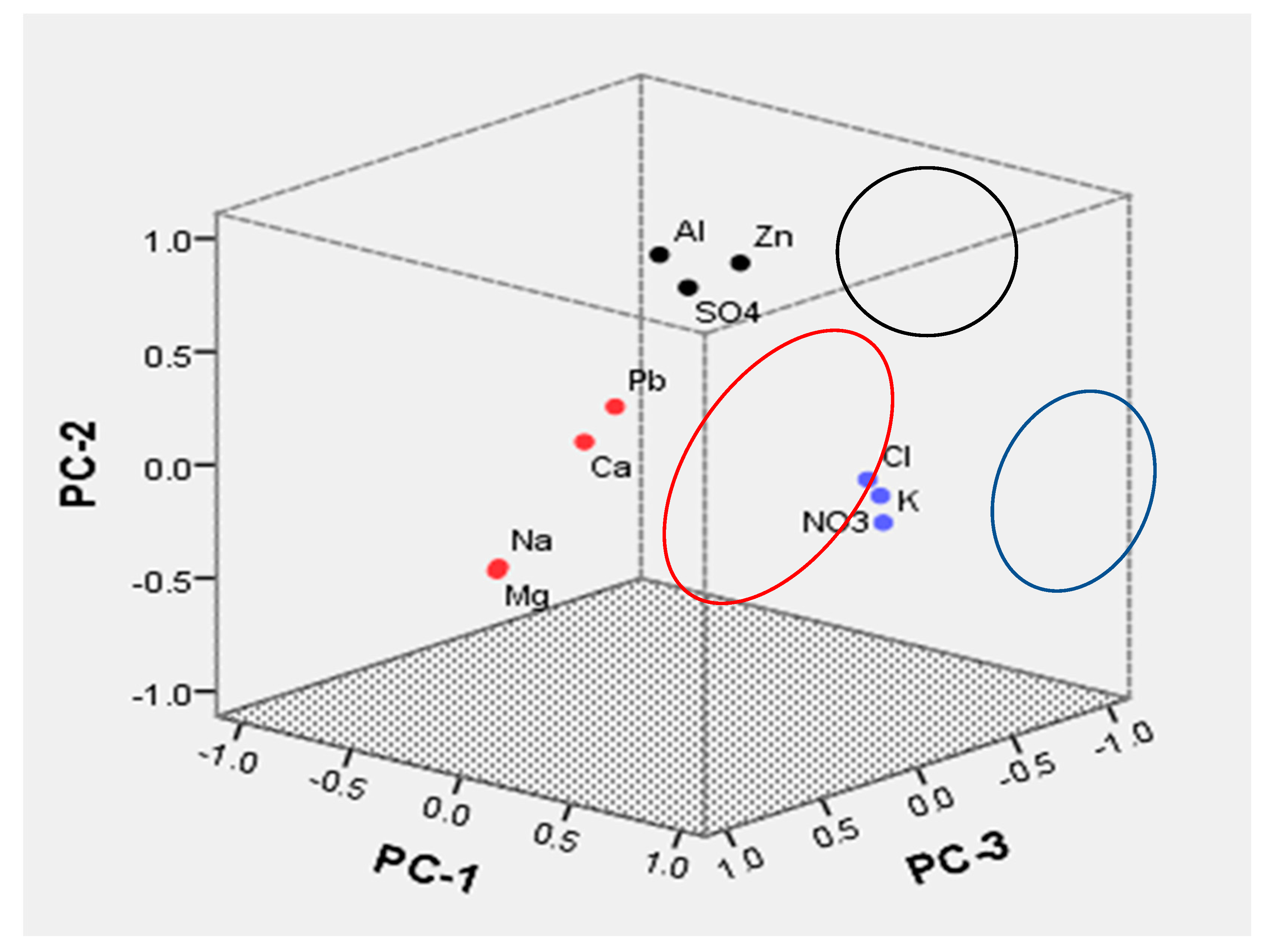
3.5.3. Principal Component Analysis

Ten independent variables were used in the principal component analysis (PCA), which produced three primary principal components (PC) that accounted for around 77.2 percent of the variation (

Table 1. Rotated component matrix after varimax rotation of ions and trace metals for present study.

Parameters	Factor 1	Factor 2	Factor 3
K+	0.98
NO3−	0.98
Cl−	0.94
SO42−		0.83
Al		0.81
Zn		0.81
Ca2+			0.75
Na+			0.89
Mg2+			0.83
Eigenvalue	3.2	2.5	1.9
Variance explained (%)	29.8	24.2	23.2
Cumulative variance (%)	29.8	54.0	77.3

) [29,32]. Principal Component 1 (PC1) had high loadings of K⁺, NO₃⁻ and Cl⁻, which together accounted for approximately 29.8% of the total variance, indicating a significant contribution from the burning of fossil fuels and biomass, as well as from vehicles. K⁺ is regarded as the marker species for biomass burning, and NO₃⁻ is thought to be a major contributor to both fossil fuel and biomass burning [10,27,58]. PC2 explained 24.2 percent of the variance with factor loadings of SO₄²⁻ Zn and Al, which are commonly emitted by industrial activities and solid waste burning. Principal Component 3 (PC3) demonstrated significant loading for Na⁺, Mg²⁺ and Ca²⁺ and is thought to be a source of crustal/soil dust resuspension [10,27,31,59,60]. The principal component analysis concluded that SO₄^−, NO₃⁻, Cl⁻ and K⁺ are anthropogenically derived (biomass burning, fossil fuel burning and vehicular emission), whereas Na⁺, Ca²⁺ and Mg²⁺ are primarily derived from crustal/soil sources. The three-dimensional rotated plot of principal component analysis is shown in Figure 8.

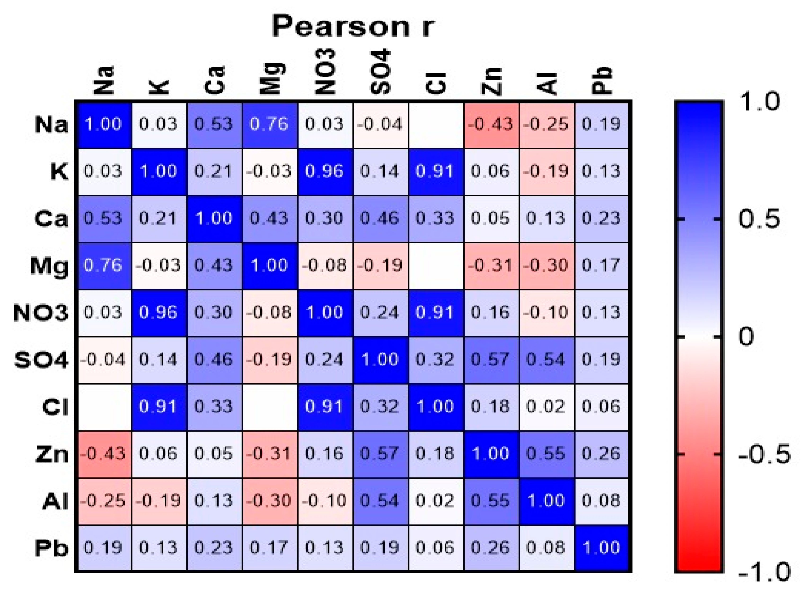
3.5.4. Multiple Correlation Analysis

For the ionic species Na⁺, K⁺, Ca²⁺, Mg²⁺, NO₃⁻, SO₄²⁻, Cl⁻, Zn, Al and Pb, many correlation tables were created. K⁺ and NO₃⁻ (r = 0.96), K⁺ and Cl⁻ (r = 0.91) and NO₃⁻ and Cl⁻ (r = 0.91) all exhibited a highly significant connection (>0.9), which indicated their presence in the form of secondary aerosols as KCl and KNO_3. This may result from the burning of plastic or biomass, whereas nitrate comes from vehicle emissions. Na⁺ and Mg²⁺ have a significant association (r = 0.76), indicating a crustal source (Figure 9).

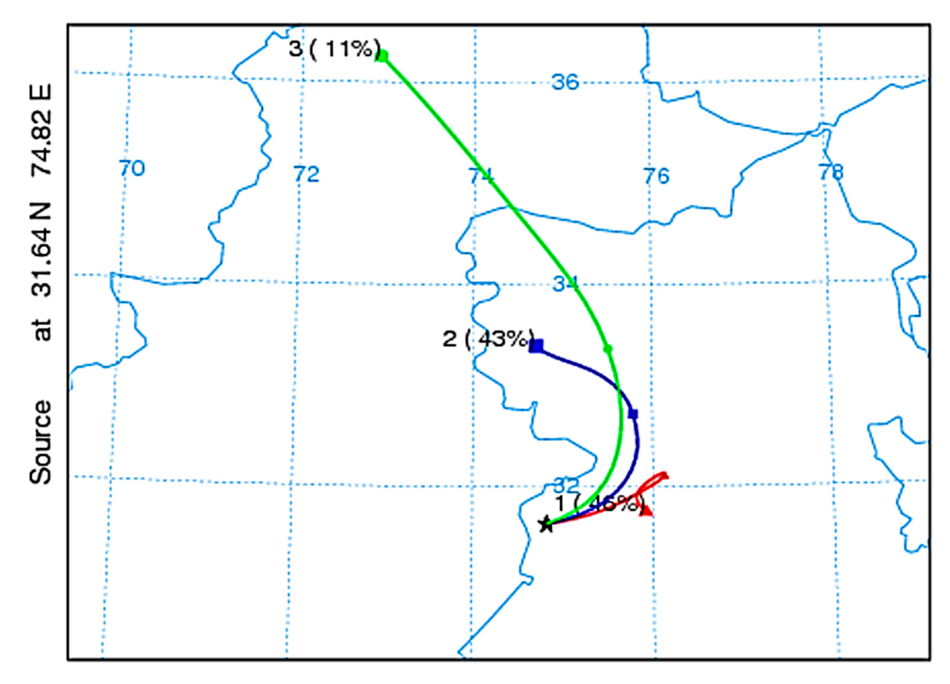
3.5.5. Air Mass Back Trajectory

HYSPLIT modeling has been investigated for air mass trajectory analysis to determine the origin of the air mass by different researchers [54,61]. For this, 24 h back trajectories starting at 500 m AGL were computed for the foggy days (n = 30, 29 December 2020 to 20 February 2021), and the pathways were clustered based on similarities in spatial distribution using the HYSPLIT model’s clustering algorithm [7]. Cluster trajectories for the entire study period show that 46 percent of the air mass originated from the north-eastern side (at a distance of 100 km from the source), and then crossed an industrial town (Batala) before reaching the study site, as depicted by cluster 1 (Figure 10). Cluster 2 originated in southern Kashmir (‘400 km from the source) and entered Amritsar from the north side. Cluster 3′s contribution is 11%, indicating long-range air mass transportation from the west side (Pakistan’s northernmost regions located approximately 1000 km from source). Separate clusters are shown in Figure S1.

It can be concluded that there was no air mass coming from the sea, and the majority of pollutants were transported from the northeast during the sampling period, which is consistent with the results of the enrichment factor analysis, with a negligible contribution from sea salts. Windrose analysis was not used in this study, but it could help to further define the prevailing wind direction and thus support the study. In summary, the majority of the contributions from the air mass trajectory (46%) came from nearby sources (100 km). A previous study conducted at the present source location reported that the air masses mainly come from the west [20].

4. Conclusions

Fog water was collected using an indigenous-made glass-plate collector. Chemical analysis of the fog water revealed a pH range of 4.6 to 7.5 and an EC range of 62 to 365 µS/cm. The ionic dominance of major ions followed the order of SO₄²⁻ (77.5 ppm) > Cl⁻ (9.9 ppm) > NO₃⁻ (9.3 ppm) > Ca²⁺ (8.1 ppm) > Mg²⁺ (2 ppm) > K⁺ (2 ppm) Na⁺ (1.6 ppm)> and trace metals Zn (218 ppb) > Al (61 ppb) > Pb (8.8 ppb). Chemical analysis indicated significant pollution from the burning of coal, solid waste, tyres and plastic waste during the sampling period. The air mass back trajectory also indicated the short-range transport of pollutants in the city, with a 46% contribution from the north-eastern region. The neutralization factor revealed that calcium and magnesium are the primary crustal components released by construction activities, as well as soil dust resuspension, in neutralizing fog water acidity, but the absence of ammonium ion data in the present study is a limitation. Enrichment factor, multiple-correlation and principal component analysis along with air mass backward trajectory techniques were used to identify the probable sources of pollution. EF indicated that all of the chemical species in the fog water had major contributions from anthropogenic sources (sulphate, nitrate, chloride and potassium), whereas primary crustal contributions were magnesium and sodium. A highly significant correlation (r > 0.9) between K⁺ and NO₃⁻ (r = 0.96), K⁺ and Cl⁻ (r = 0.91) and NO₃⁻ and Cl⁻ (r = 0.91) indicates the presence of secondary inorganic aerosols such as KCl and KNO₃ in the atmosphere. A significant correlation between nitrate and chloride (both anions) reveals a phase change between particulate nitrate and chloride. This pathway is more predominant at the high relative humidity and acidic pH of the fog water. PCA shows that the primary principal component (PC-1) comprises K⁺, NO₃⁻ and Cl⁻, again revealing significant burning activities. The SO₄²⁻/NO₃⁻ ratio is useful when their ionic concentration is significant (>10 ppm). Meteorological phenomena are complex and need simultaneous measurements to check the contributions of ionic constituents in the formation of ozone or secondary organic aerosols. Advanced instrumentation techniques such as chemical ionization mass spectrophotometry may be useful in future studies.

Future studies may be directed towards simultaneous measurements of aerosols and fog water during the day and night to study the effect of light on the generation of secondary aerosols. A geographical comparison of fog water for sulphate, chloride, nitrate, magnesium, calcium, potassium, sodium, aluminum, lead and zinc showed that the nitrate and sodium concentrations in the present study were the lowest among different studies. However, this should be interpreted with caution as these pollutants may activate other pollutants, such as volatile organic compounds, and generate free radicals in the environment when the other conditions such as RH and pH are more conducive.

References

1. Guo, B.; Wang, Y.; Zhang, X.; Che, H.; Zhong, J.; Chu, Y.; Cheng, L. Temporal and spatial variations of haze and fog and the characteristics of PM2.5 during heavy pollution episodes in China from 2013 to 2018. Atmos. Pollut. Res. 2020, 11, 1847–1856. [Google Scholar] [CrossRef]
2. Dutta, D.; Chaudhuri, S. Nowcasting visibility during wintertime fog over the airport of a metropolis of India: Decision tree algorithm and artificial neural network approach. Nat. Hazards 2015, 75, 1349–1368. [Google Scholar] [CrossRef]
3. Ivanov, O.; Todorov, P.; Gultepe, I. Investigations on the influence of chemical compounds on fog microphysical parameters. Atmosphere 2020, 11, 225. [Google Scholar] [CrossRef]
4. Chen, K.; Yin, Y.; Hu, Z. Influence of air pollutants on fog formation in urban environment of Nanjing, China. Procedia Eng. 2011, 24, 654–657. [Google Scholar] [CrossRef]
5. Mohan, M.; Payra, S. Influence of aerosol spectrum and air pollutants on fog formation in urban environment of megacity Delhi, India. Environ. Monit. Assess. 2009, 151, 265–277. [Google Scholar] [CrossRef] [PubMed]
6. Yan, S.; Zhu, B.; Huang, Y.; Zhu, J.; Kang, H.; Lu, C.; Zhu, T. To what extents do urbanization and air pollution affect fog? Atmos. Chem. Phys. 2020, 20, 5559–5572. [Google Scholar] [CrossRef]
7. Izhar, S.; Gupta, T.; Minz, A.P.; Senapati, S.; Panday, A.K. Influence of regional and long range transport air masses on fog water composition, contribution and toxicological response at Indo Gangetic Plain. Atmos. Environ. 2019, 214, 116888. [Google Scholar] [CrossRef]
8. Ghude, S.D.; Bhat, G.S.; Prabhakaran, T.; Jenamani, R.K.; Chate, D.M.; Safai, P.D.; Karipot, A.K.; Konwar, M.; Pithani, P.; Sinha, V.; et al. Winter fog experiment over the Indo-Gangetic plains of India. Curr. Sci. 2017, 112, 767–784. [Google Scholar] [CrossRef]
9. Nair, V.S.; Moorthy, K.K.; Alappattu, D.P.; Kunhikrishnan, P.K.; George, S.; Nair, P.R.; Babu, S.S.; Abish, B.; Satheesh, S.K.; Tripathi, S.N. Wintertime aerosol characteristics over the Indo-Gangetic Plain (IGP): Impacts of local boundary layer processes and long-range transport. J. Geophys. Res. Atmos. 2007, 112, D13205. [Google Scholar] [CrossRef]
10. Wang, W.; Xu, W.; Collett, J.L., Jr.; Liu, D.; Zheng, A.; Dore, A.J.; Liu, X. Chemical compositions of fog and precipitation at Sejila Mountain in the southeast Tibetan Plateau, China. Environ. Pollut. 2019, 253, 560–568. [Google Scholar] [CrossRef] [PubMed]
11. Li, W.; Wang, Y.; Collett, J.L., Jr.; Chen, J.; Zhang, X.; Wang, Z.; Wang, W. Microscopic evaluation of trace metals in cloud droplets in an acid precipitation region. Environ. Sci. Technol. 2013, 47, 4172–4180. [Google Scholar] [CrossRef]
12. Bianco, A.; Vaïtilingom, M.; Bridoux, M.; Chaumerliac, N.; Pichon, J.M.; Piro, J.L.; Deguillaume, L. Trace metals in cloud water sampled at the puy de Dôme station. Atmosphere 2017, 8, 225. [Google Scholar] [CrossRef]
13. Yang, Y.; Ge, B.; Chen, X.; Yang, W.; Wang, Z.; Chen, H.; Xu, D.; Wang, J.; Tan, Q.; Wang, Z. Impact of water vapor content on visibility: Fog-haze conversion and its implications to pollution control. Atmos. Res. 2021, 256, 105565. [Google Scholar] [CrossRef]
14. Wang, Y.; Okochi, H.; Igawa, M. Characteristics of fog and fog collection with passive Collector at Mt. Oyama in Japan. Water Air Soil Pollut. 2021, 232, 260. [Google Scholar] [CrossRef]
15. Liu, Z.; Wang, H.; Peng, Y.; Zhang, W.; Zhao, M. Multiple Regression Analysis of low visibility focusing on severe haze-fog pollution in various regions of China. Atmosphere 2022, 13, 203. [Google Scholar] [CrossRef]
16. Carvajal, D.; Mora-Carreño, M.; Sandoval, C.; Espinoza, S. Assessing fog water collection in the coastal mountain range of Antofagasta, Chile. J. Arid. Environ. 2022, 198, 104679. [Google Scholar] [CrossRef]
17. Liu, X.H.; Wai, K.M.; Wang, Y.; Zhou, J.; Li, P.H.; Guo, J.; Xu, P.J.; Wang, W.X. Evaluation of trace elements contamination in cloud/fog water at an elevated mountain site in Northern China. Chemosphere 2012, 88, 531–541. [Google Scholar] [CrossRef]
18. Kumar, S.; Nath, S.; Bhatti, M.S.; Yadav, S. Chemical characteristics of fine and coarse particles during wintertime over two urban cities in North India. Aerosol Air Qual. Res. 2018, 18, 1573–1590. [Google Scholar] [CrossRef]
19. Ravindra, K.; Singh, T.; Mor, S.; Singh, V.; Mandal, T.K.; Bhatti, M.S.; Gahlawat, S.K.; Dhankar, R.; Mor, S.; Beig, G. Real-time monitoring of air pollutants in seven cities of North India during crop residue burning and their relationship with meteorology and transboundary movement of air. Sci. Total Environ. 2019, 690, 717–729. [Google Scholar] [CrossRef] [PubMed]
20. Yadav, R.; Bhatti, M.S.; Kansal, S.K.; Das, L.; Gilhotra, V.; Sugha, A.; Sugha, A.; Hingmire, D.; Yadav, S.; Tandon, A.; et al. Comparison of ambient air pollution levels of Amritsar during foggy conditions with that of five major north Indian cities: Multivariate analysis and air mass back trajectories. SN Appl. Sci. 2020, 2, 1761. [Google Scholar] [CrossRef]
21. Nahar, K.; Nahian, S.; Jeba, F.; Islam, M.S.; Rahman, M.S.; Choudhury, T.R.; Fatema, K.J.; Salam, A. Characterization and Source Discovery of Wintertime Fog on Coastal Island, Bangladesh. Atmosphere 2022, 13, 497. [Google Scholar] [CrossRef]
22. Kumar, P.; Yadav, S. Factors and sources influencing ionic composition of atmospheric condensate during winter season in lower troposphere over Delhi, India. Environ. Monit. Assess. 2013, 185, 2795–2805. [Google Scholar] [CrossRef] [PubMed]
23. Yadav, R.; Sugha, A.; Bhatti, M.S.; Kansal, S.K.; Sharma, S.K.; Mandal, T.K. The role of particulate matter in reduced visibility and anionic composition of winter fog: A case study for Amritsar city. RSC Adv. 2022, 12, 11104–11112. [Google Scholar] [CrossRef] [PubMed]
24. Baird, R.B.; Eaton, A.D.; Rice, E.W. (Eds.) Standard Methods for the Examination of Water and Wastewater, 23rd ed.; American Public Health Association (APHA): Washington, DC, USA, 2017. [Google Scholar]
25. Ali, K.; Momin, G.A.; Tiwari, S.; Safai, P.D.; Chate, D.M.; Rao, P.S.P. Fog and precipitation chemistry at Delhi, North India. Atmos. Environ. 2004, 38, 4215–4222. [Google Scholar] [CrossRef]
26. Simon, S.; Klemm, O.; El-Madany, T.; Walk, J.; Amelung, K.; Lin, P.H.; Chang, S.C.; Lin, N.H.; Engling, G.; Hsu, S.C.; et al. Chemical composition of fog water at four sites in Taiwan. Aerosol Air Qual. Res. 2016, 16, 618–631. [Google Scholar] [CrossRef]
27. Bisht, D.S.; Srivastava, A.K.; Joshi, H.; Ram, K.; Singh, N.; Naja, M.; Tiwari, S. Chemical characterization of rainwater at a high-altitude site “Nainital” in the central Himalayas, India. Environ. Sci. Pollut. Res. 2017, 24, 3959–3969. [Google Scholar] [CrossRef] [PubMed]
28. Shohel, M.; Simol, H.A.; Reid, E.; Reid, J.S.; Salam, A. Dew water chemical composition and source characterization in the IGP outflow location (coastal Bhola, Bangladesh). Air Qual. Atmos. Health 2017, 10, 981–990. [Google Scholar] [CrossRef]
29. Cao, Y.Z.; Wang, S.; Zhang, G.; Luo, J.; Lu, S. Chemical characteristics of wet precipitation at an urban site of Guangzhou, South China. Atmos. Res. 2009, 94, 462–469. [Google Scholar] [CrossRef]
30. Lu, X.; Li, L.Y.; Li, N.; Yang, G.; Luo, D.; Chen, J. Chemical characteristics of spring rainwater of Xi’an city, NW China. Atmos. Environ. 2011, 45, 5058–5063. [Google Scholar] [CrossRef]
31. Liu, Y.W.; Ri, X.; Wang, Y.S.; Pan, Y.P.; Piao, S.L. Wet deposition of atmospheric inorganic nitrogen at five remote sites in the Tibetan Plateau. Atmos. Chem. Phys. 2015, 15, 11683–11700. [Google Scholar] [CrossRef] [Green Version]
32. Singh, K.P.; Singh, V.K.; Malik, A.; Sharma, N.; Murthy, R.C.; Kumar, R. Hydrochemistry of wet atmospheric precipitation over an urban area in Northern Indo-Gangetic Plains. Environ. Monit. Assess. 2007, 131, 237–254. [Google Scholar] [CrossRef]
33. Lakhani, A.; Parmar, R.S.; Satsangi, G.S.; Prakash, S. Chemistry of fogs at Agra, India: Influence of soil particulates and atmospheric gases. Environ. Monit. Assess. 2007, 133, 435–445. [Google Scholar] [CrossRef]
34. Lekouch, I.; Muselli, M.; Kabbachi, B.; Ouazzani, J.; Melnytchouk-Milimouk, I.; Beysens, D. Dew, fog, and rain as supplementary sources of water in south-western Morocco. Energy 2011, 36, 2257–2265. [Google Scholar] [CrossRef]
35. Beysens, D.; Ohayon, C.; Muselli, M.; Clus, O. Chemical and biological characteristics of dew and rain water in an urban coastal area (Bordeaux, France). Atmos. Environ. 2006, 40, 3710–3723. [Google Scholar] [CrossRef]
36. Kaul, D.S.; Gupta, T.; Tripathi, S.N.; Tare, V.; Collett, J.L., Jr. Secondary organic aerosol: A comparison between foggy and nonfoggy days. Environ. Sci. Technol. 2011, 45, 7307–7313. [Google Scholar] [CrossRef]
37. Boris, A.J.; Napolitano, D.C.; Herckes, P.; Clements, A.L.; Collett, J.L., Jr. Fogs and air quality on the southern California coast. Aerosol Air Qual. Res. 2018, 18, 224–239. [Google Scholar] [CrossRef]
38. Mishra, M.; Kulshrestha, U.C. Extreme air pollution events spiking ionic levels at urban and rural sites of Indo-Gangetic plain. Aerosol Air Qual. Res. 2020, 20, 1266–1281. [Google Scholar] [CrossRef]
39. Nath, S.; Yadav, S. A comparative study on fog and dew water chemistry at New Delhi, India. Aerosol Air Qual. Res. 2018, 18, 26–36. [Google Scholar] [CrossRef]
40. Ambade, B. Characterization and source of fog water contaminants in central India. Nat. Hazards 2014, 70, 1535–1552. [Google Scholar] [CrossRef]
41. Li, P.; Li, X.; Yang, C.; Wang, X.; Chen, J.; Collett, J.L., Jr. Fog water chemistry in Shanghai. Atmos. Environ. 2011, 45, 4034–4041. [Google Scholar] [CrossRef]
42. Błaś, M.; Polkowska, Ż.; Sobik, M.; Klimaszewska, K.; Nowiński, K.; Namieśnik, J. Fog water chemical composition in different geographic regions of Poland. Atmos. Res. 2010, 95, 455–469. [Google Scholar] [CrossRef]
43. Lu, C.; Niu, S.; Tang, L.; Lv, J.; Zhao, L.; Zhu, B. Chemical composition of fog water in Nanjing area of China and its related fog microphysics. Atmos. Res. 2010, 97, 47–69. [Google Scholar] [CrossRef]
44. Wang, Y.; Zhang, J.; Marcotte, A.R.; Karl, M.; Dye, C.; Herckes, P. Fog chemistry at three sites in Norway. Atmos. Res. 2015, 151, 72–81. [Google Scholar] [CrossRef]
45. Xu, X.; Chen, J.; Zhu, C.; Li, J.; Sui, X.; Liu, L.; Sun, J. Fog composition along the Yangtze River basin: Detecting emission sources of pollutants in fog water. J. Environ. Sci. 2018, 71, 2–12. [Google Scholar] [CrossRef]
46. Beiderwieden, E.; Wrzesinsky, T.; Klemm, O. Chemical characterization of fog and rain water collected at the eastern Andes cordillera. Hydrol. Earth Syst. Sci. 2005, 9, 185–191. [Google Scholar] [CrossRef]
47. Kim, M.G.; Lee, B.K.; Kim, H.J. Cloud/fog water chemistry at a high elevation site in South Korea. J. Atmos. Chem. 2006, 55, 13–29. [Google Scholar] [CrossRef]
48. Nieberding, F.; Breuer, B.; Braeckevelt, E.; Klemm, O.; Song, Q.; Zhang, Y. Fog water chemical composition on ailaoshan mountain, Yunnan province, SW China. Aerosol Air Qual. Res. 2018, 18, 37–48. [Google Scholar] [CrossRef]
49. Boris, A.J.; Lee, T.; Park, T.; Choi, J.; Seo, S.J.; Collett, J.L., Jr. Fog composition at Baengnyeong Island in the eastern Yellow Sea: Detecting markers of aqueous atmospheric oxidations. Atmos. Chem. Phys. 2016, 16, 437–453. [Google Scholar] [CrossRef]
50. Straub, D.J.; Hutchings, J.W.; Herckes, P. Measurements of fog composition at a rural site. Atmos. Environ. 2012, 47, 195–205. [Google Scholar] [CrossRef]
51. Sheoran, R.; Dumka, U.C.; Sowmya, H.N.; Bisht, D.S.; Srivastava, A.K.; Tiwari, S.; Attri, S.D.; Hopke, P.K. Changes in inorganic chemical species in fog water over Delhi. Asian J. Atmos. Environ. 2022, 16, 2021092. [Google Scholar] [CrossRef]
52. Li, T.; Wang, Z.; Wang, Y.; Wu, C.; Liang, Y.; Xia, M.; Yu, C.; Yun, H.; Wang, W.; Wang, Y.; et al. Chemical characteristics of cloud water and the impacts on aerosol properties at a subtropical mountain site in Hong Kong SAR. Atmos. Chem. Phys. 2020, 20, 391–407. [Google Scholar] [CrossRef]
53. IS-10500; Indian Standards-Drinking Water Specifications. Bureau of Indian Standards: New Delhi, India, 2012.
54. Hutchings, J.W.; Robinson, M.S.; McIlwraith, H.; Triplett Kingston, J.; Herckes, P. The chemistry of intercepted clouds in Northern Arizona during the North American monsoon season. Water Air Soil Pollut. 2009, 199, 191–202. [Google Scholar] [CrossRef]
55. Keene, W.C.; Pszenny, A.A.; Galloway, J.N.; Hawley, M.E. Sea-salt corrections and interpretation of constituent ratios in marine precipitation. Journal of Geophysical Research: Atmospheres. 1986, 91, 6647–6658. [Google Scholar] [CrossRef]
56. Rao, P.S.P.; Tiwari, S.; Matwale, J.L.; Pervez, S.; Tunved, P.; Safai, P.D.; Srivastava, A.K.; Bisht, D.S.; Singh, S.; Hopke, P.K. Sources of chemical species in rainwater during monsoon and non-monsoonal periods over two mega cities in India and dominant source region of secondary aerosols. Atmospheric Environment. 2016, 146, 90–99. [Google Scholar] [CrossRef]
57. Yadav, S.; Kumar, P. Pollutant scavenging in dew water collected from an urban environment and related implications. Air Quality, Atmosphere Health 2014, 7, 559–566. [Google Scholar] [CrossRef]
58. Gobre, T.; Salve, P.R.; Krupadam, R.J.; Bansiwal, A.; Shastry, S.; Wate, S.R. Chemical composition of precipitation in the coastal environment of India. Bull. Environ. Contam. Toxicol. 2010, 85, 48–53. [Google Scholar] [CrossRef]
59. Zhang, M.; Wang, S.; Wu, F.; Yuan, X.; Zhang, Y. Chemical compositions of wet precipitation and anthropogenic influences at a developing urban site in southeastern China. Atmos. Res. 2007, 84, 311–322. [Google Scholar] [CrossRef]
60. Momin, G.A.; Ali, K.; Rao, P.S.P.; Safai, P.D.; Chate, D.M.; Praveen, P.S.; Rodhe, H.; Granat, L. Study of chemical composition of rainwater at an urban (Pune) and a rural (Sinhagad) location in India. J. Geophys. Res. 2005, 110, D08302. [Google Scholar] [CrossRef]
61. Prabhu, V.; Prakash, J.; Soni, A.; Madhwal, S.; Shridhar, V. Atmospheric aerosols and inhalable particle number count during Diwali in Dehradun. City Environ. Interact. 2019, 2, 100006. [Google Scholar] [CrossRef]
Figure 1. Sampling site in Amritsar city.
Atmosphere 13 01376 g001
Figure 2. Global perspective of (a) pH and (b) conductivity in fog water studies (reproduced and modified with permission from [23]. References included are [8,17,23,33,34,35,36,37,38,39,40,41,42,43,44,45,46,47,48,49,50].
Atmosphere 13 01376 g002
Figure 3. Box plot showing ions in fog water from Dec. 2020 to Feb. 2021. Box in the figure shows the interquartile range, the star shows outliers, the line shows the median, and the small square box is the mean (n = 26 samples).
Atmosphere 13 01376 g003
Figure 4. Review graph of anionic concentration (mg/L) on normalized scale (0.5–1.5) for chloride (red), sulphate (green) and nitrate (blue) in fog water studies, (Black color represent own study). References included are [23,33,39,40,51].
Atmosphere 13 01376 g004
Figure 5. Review graph of cationic concentration (mg/L) on normalized scale (0.5–1.5) for magnesium (red), calcium (green), potassium (blue) and sodium (yellow) in fog water studies, (Black color represent own study). References included are [33,39,40,51].
Atmosphere 13 01376 g005
Figure 6. Review graph of metal concentrations (ppb) on normalized scale (0.5–1.5) for aluminum (red), lead (green) and zinc (blue) in fog water studies, (Black color represent own study). References included are [10,11,12,17,21,26,32,40,50,52,54].
Atmosphere 13 01376 g006
Figure 7. Stacked graph for sulphate and nitrate concentration along with sulphate to nitrate ratio in fog water. References included are [8,23,25,51].
Atmosphere 13 01376 g007
Figure 8. Factor loading plot in three-dimensional rotated space for ions and trace metals in present study. PC-1 (blue circle), PC-2 (black circle) and PC-3 (red circle).
Atmosphere 13 01376 g008
Figure 9. Pearson correlation matrix between ions and trace metals in fog water for present study.
Atmosphere 13 01376 g009
Figure 10. Cluster analysis of air mass back trajectories calculated at a height of 500 m above ground level for sampling days. Cluster 1 showing 46% contribution (red line), Cluster 2 showing 43% contribution (blue line) and Cluster 3 showing 11% contribution (green line) in origin of air masses.
Atmosphere 13 01376 g010