Max Fast Fourier Transform (maxFFT) Clustering Approach for Classifying Indoor Air Quality

Abstract

Air pollution is a severe problem for the global environment. Most people spend 80% to 90% of the day indoors; therefore, indoor air pollution is as important as outdoor air pollution. The problem is more severe on school campuses. There are several ways to improve indoor air quality, such as air cleaners or ventilation. Air-quality sensors can be used to detect indoor air quality in real time to turn on air cleaner or ventilation. With an efficient and accurate clustering technique for indoor air-quality data, different ventilation strategies can be applied to achieve a better ventilation policy with accurate prediction results to improve indoor air quality. This study aims to cluster the indoor air quality data (i.e., CO₂ level) collected from the school campus in Taiwan without other external information, such as geographical location or field usage. In this paper, we propose the Max Fast Fourier Transform (maxFFT) Clustering Approach to classify indoor air quality to improve the efficiency of the clustering and extract the required feature. The results show that without using geographical information or field usage, the clustering results can correctly reflect the ventilation condition of the space with low computation time.

1. Introduction

1.1. Background

Pollution is a global problem, especially in urban areas. Air pollution, water pollution, and land pollution are three major types of pollution that are usually created by humans. Although people can elect to drink bottled water or live in a more suitable area, one cannot choose or stop breathing the air surrounding them. In fact, according to the World Health Organization (WHO) [1], 4.2 million deaths were due to exposure to ambient air pollution in 2016. These show that air has a significant impact on the human body.

Most people spend 80% to 90% of the day indoors [2]; therefore, indoor air pollution is as important as outdoor air pollution. According to the U.S. Environmental Protection Agency (EPA) [3], indoor air quality is often 2 to 5 times worse than the outdoor air quality. This indicates that the effects of indoor air on the human body may be larger than those of the outdoor air. However, indoor air quality has not been studied as much as outdoor air quality in the past [4].

1.2. Literature Review

Clustering [5] is a form of statistical analysis that aims to classify data with similar characteristics into the same group. Similarity needs to be evaluated regardless of the characteristics. One of the most common evaluation methods is to use Euclidean distance [6] as a similarity measurement. The Euclidean distance between two points in one dimension is the absolute value of the numerical difference in their coordinates.

Take the iris flower data set (also known as Fisher’s iris data set) [7], for example. It contains sepal length, sepal width, petal length, petal width, and species. There are three species of the iris in the data set (iris setosa, iris virginica, and iris versicolor), each with 50 samples. Chakraborty et al. [8] evaluated four different similarity measurements (Euclidean distance, Manhattan distance, Cosine similarity, and Correlation distance metrics) on sepal and petal size and concluded that species accuracy on K-means clustering by sepal and petal was at least 90%, and it reached up to 98% on the iris data set.

Clustering has been used widely in air-quality analysis. Methods include K-means [9,10,11], gray clustering [12,13], or K-medoids [14]. Caron et al. [9] used K-means clustering with two data sets to identify air-quality events with two measurements. One is reference online analyzer measurements, and the other is electrochemical and nondispersive infrared sensor measurements. The number of clusters for both data sets is from 2 to 10. The overlap ratios of two clustering results (with five classes) are at least 87.6% and reach up to 98.4%.

Sunori et al. [10] investigated with two distance measuring approaches (Euclidean distance and cosine distance) in K-means. They mixed Indian air-quality data (PM₁₀, SO₂, and NO₂) of two years in 2020 (during the lockdown period of COVID-19) and the preceding year, 2019. After applying cluster analysis, they concluded that the Euclidean distance approach obtains a better clustering result than cosine distance for two-year mixed data. Chen et al. [11] present an algorithm called EPLS based on Ensemble Empirical Mode Decomposition (EEMD), Principal Component Analysis (PCA), and Least Square method (LS). The EPLS can extract features from the original time series data for clustering. The result shows that EPLS clustering is slightly superior to raw data clustering with k-means and distance measures on cluster time series data. Zhu and Li [12] used gray clustering to simplify the indicators of indoor air quality. They chose office buildings in two of China’s cities as case studies. The results show that out of all seven measured pollutants, CO₂, respirable particulate (RSP), and formaldehyde (HCHO) are indicators of indoor air quality.

Time series clustering has been extensively applied in different domains [15], such as finance, biology, climate [16,17], and environment. In general, there are three different ways to cluster time series data, i.e., Shape-based, Feature-based, and Model-based methods. Shaped-based means clustering is based on shapes’ similarity. Feature-based extraction methods feature(s) occur from raw data to clustering. Model-based methods transform raw data into parametric model parameters before clustering.

Li et al. [18] proposed a generic framework for anomaly detection on amplitude and shapes through an extended version of the Fuzzy C-Means clustering. Dincer and Özge Akkuşs [16] proposed a fuzzy time series model based on a Fuzzy K-Medoids clustering algorithm to forecast air pollution (SO₂ concentration). They conclude that the model predicts success, especially in time series that contain numerous outliers.

Alahamade et al. [17] proposed a method to impute missing data for the whole time series via multivariate time series (MVTS). They chose three years (2015∼2017) as a training set and selected alternate years (2018) as the test set for imputation. On time series variables including O₃, NO₂, PM₁₀, and PM_2.5 data, K-means were selected for clustering, and similarity was measured by shape-based distance. They proposed two methods to impute missing data. One is the same cluster average (CA) value, and the other is the average from the same cluster and the same environment type (CA+ENV). The results show better (lower) root-mean-square error (RMSE) on both univariate and multi-variate clustering for imputing NO₂ and O₃ with CA+ENV, and PM_2.5 and PM₁₀ with CA.

1.3. Motivation

Past studies on the causes of indoor air pollution focused on two areas: producing and removing pollutants. Typical indoor pollutants generated from our daily necessities include volatile organic compounds (VOCs), carbon monoxide (CO), particulate matter (PM), and radon (Rn). VOCs are evaporated from paints, cleaning supplies, disinfectants, and other solvents which may cause eye, nose, throat irritation, and headaches [19]. CO is produced from incomplete oxidation during combustion in gas ranges or kerosene heaters, which is potentially fatal in high concentrations. Indoor PM mainly migrates from an outdoor origin or indoor sources, such as cooking and tobacco smoking, which can cause respiratory illnesses [20]. Radon is released from building materials such as marble or soil, and this is one of the main causes of lung cancer among non-smokers [21]. In addition, the indoor microbial concentrations of airborne bacteria and fungi are necessary to estimate the health hazard. Those indoor pollutants and microbial concentrations are harmful to humans.

Compared to VOCs and PM, carbon dioxide (CO₂) is less harmful to humans. However, it is still an inescapable problem. Most of the indoor CO₂ is exhausted by the occupants. With insufficient ventilation, the indoor CO₂ concentration will continue to accumulate. Therefore, CO₂ concentration can indicate indoor air ventilation levels or indoor air quality [12,22,23]. A higher concentration of CO₂ in the indoor environment may decrease the decision-making performance or the cognitive performance of humans [24,25]. Therefore, ventilation for CO₂ is a serious issue for indoor air quality.

In addition to indoor pollutants, microbial concentration is another index for indoor air quality. In [26], the authors conducted a microbiological quality assessment study to determine the microbial diversity (i.e., bacterial and fungal cultures) in a historic wooden church. A subjective assessment of indoor air quality using the focus group method revealed that individuals who are undertaking their activity inside the wooden church perceive rather good indoor air quality. Fungi can also attach to different objects. In [27], a case study of artifacts from Maramures, Romania. Fungi on heritage objects can have harmful effects on people (e.g., restorers, museographers, collectors, or visitors) who come in contact with such infested objects and can develop specific conditions. The paper investigated the types of fungi present on the objects which are determined primarily through the open plates technique and microscopic identification.

According to EPA [3], there are several ways to improve indoor air quality, such as reducing the use of cleaning products that contain irritant ingredients, using air purifiers with high-efficiency particulate air (HEPA) filters to capture pollutants in the air, and enhancing ventilation with clean outdoor air to remove CO, CO₂, and Rn. In general, the ways to improve indoor air quality are (1) source control, (2) air cleaners, and (3) improved ventilation. Ventilation is the most effective way to improve indoor air quality.

In general, ventilation can be divided into passive ventilation and active ventilation. Passive ventilation, also known as natural ventilation, is achieved through natural physical characteristics, such as using thermal buoyancy and wind to enhance ventilation. On the other hand, active ventilation, such as Heating, Ventilation, and Air Conditioning (HVAC) systems, is very common in most modern buildings, enhancing ventilation and thermal comfort. Generally speaking, both types of ventilation can improve indoor air quality by bringing fresh air from the outdoors into the building.

Ventilation requirements are different in various physical settings. We observed various CO₂ concentration trends in various physical settings, such as floor level, room size, or the number and size of windows. Different ventilation strategies are needed based on different surroundings. With efficient and accurate clustering techniques on indoor CO₂ concentration trends, different strategies can be applied to achieve a better ventilation policy with accurate prediction results.

1.4. Contributions of the Research

This paper proposed a clustering method called Max Fast Fourier Transform (maxFFT), based on the fast Fourier transform to classify field types using indoor air-quality data (i.e., CO₂) without the need to use any additional information, e.g., environmental conditions, location, or the number of people. With classified field types, we can choose different ventilation strategies to improve indoor air quality to provide occupants with better indoor sensation.

The remaining sections are structured as follows. Section 2 discusses the data collection process and data preprocessing. The proposed Max Fast Fourier Transform (maxFFT) clustering approach for classifying indoor air quality is introduced. Our experimental results and discussion are presented in Section 3. Finally, we draw our conclusions and discussions in Section 4.

2. Materials and Methods

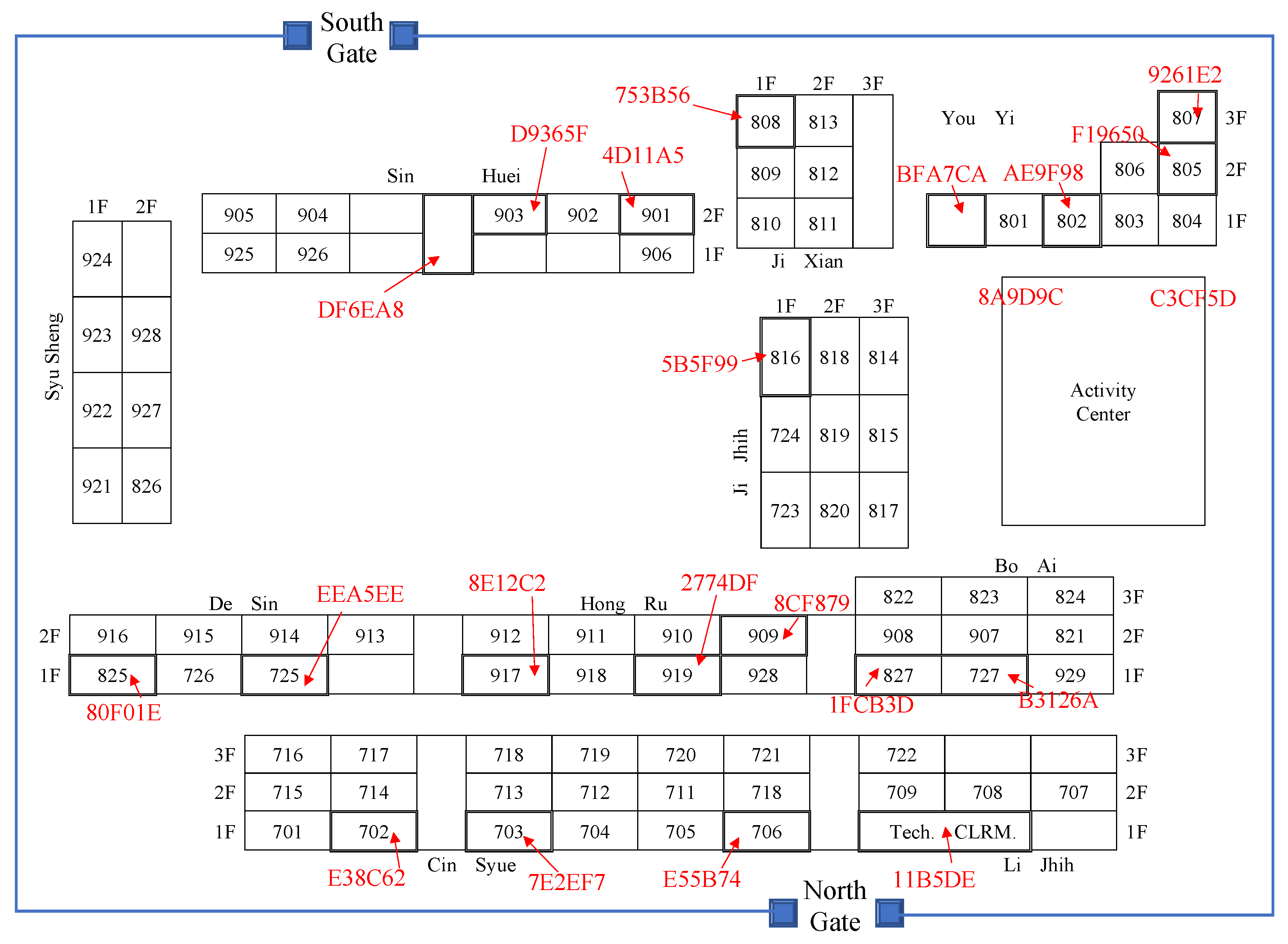
2.1. Study Area

All airboxes [28,29] used in this paper were installed in Taoyuan Municipal Neili Junior High School in Taiwan. The school had approximately 2500 students in 2019. There is an electronics manufacturer next to it and an industrial area nearby. Figure 1 is the campus map. All buildings have a varying number of airboxes installed, except for the building located on the left-hand side of the map. All 22 airboxes are installed in 21 spaces in 10 buildings. We installed two airboxes in the activity center, one airbox (DF6EA8) in the corridor, and other airboxes in classrooms of different grades and purposes of usage.

The data collection time was 261 days (37 weeks) from August 2020 to April 2021, as in Figure 2. The season is from summer to the following spring. There was a total of 814 devices per week of data (i.e., 22 airboxes × 37 weeks) if there were no missing values. Due to sensor anomaly and power instability, only 764 devices per week of data are used for our study.

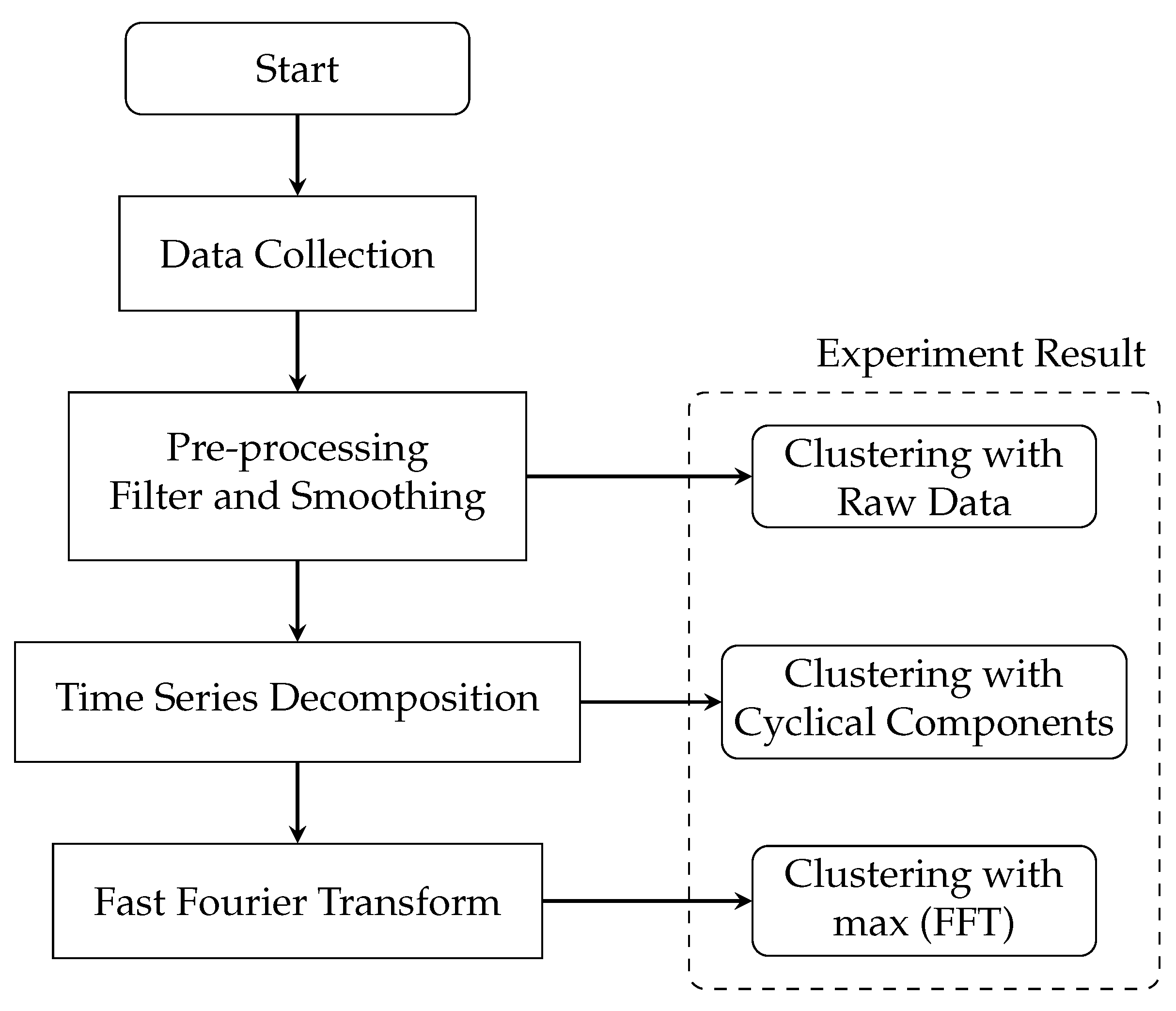
2.2. Overview of Maxfft

After the data were collected, the proposed MaxFFT clustering comprised several steps, including preprocessing, time series decomposing, fast Fourier transfer, and K-means clustering as shown in Figure 3. We will discuss each step in the following sections.

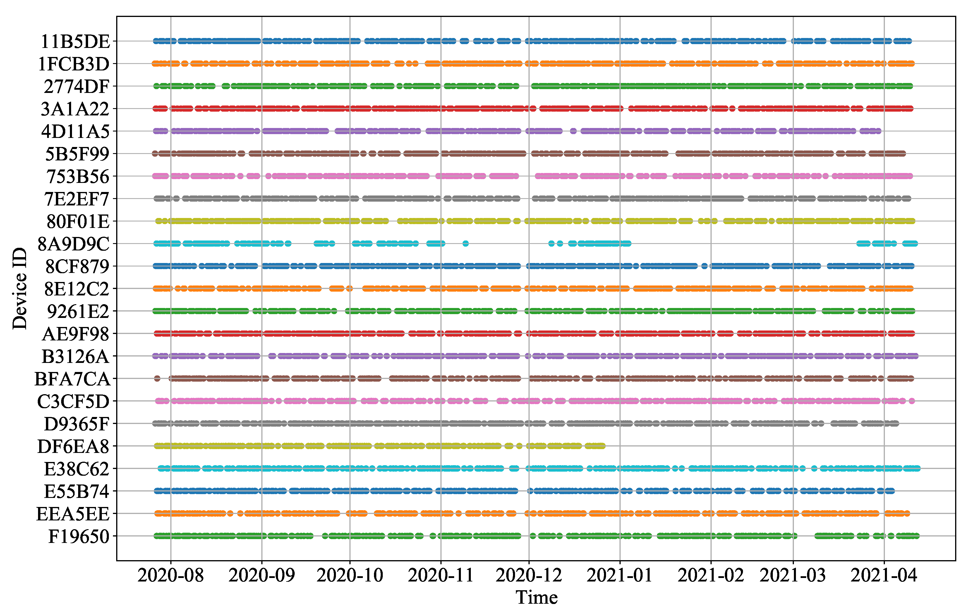
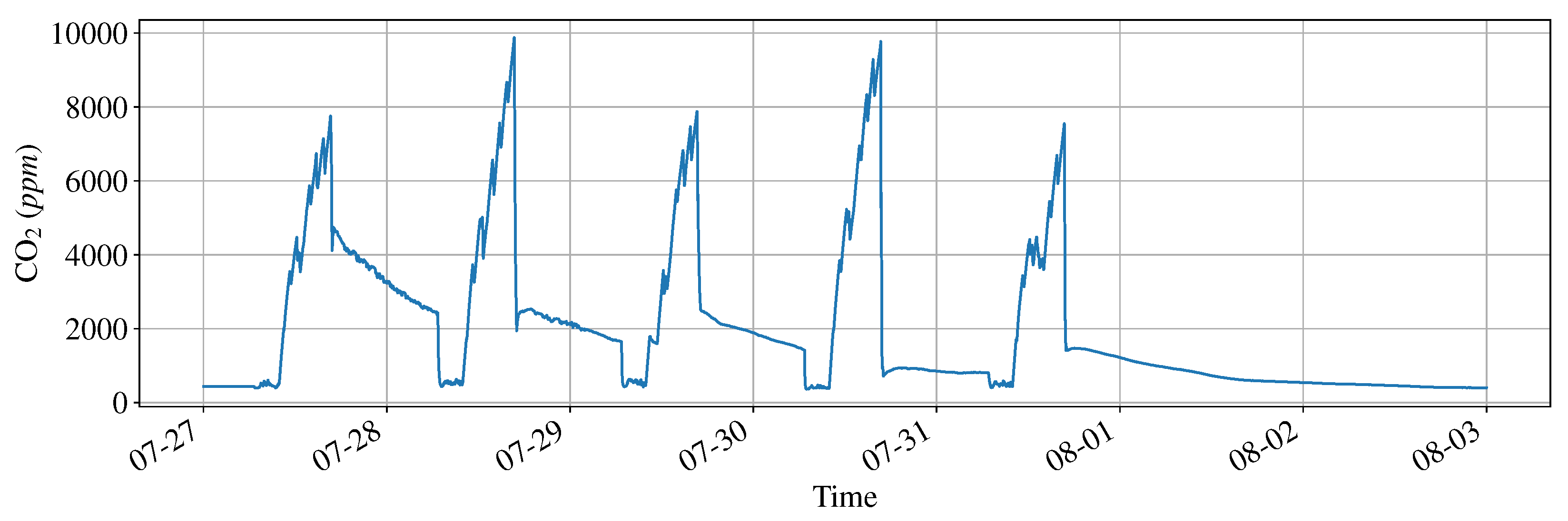
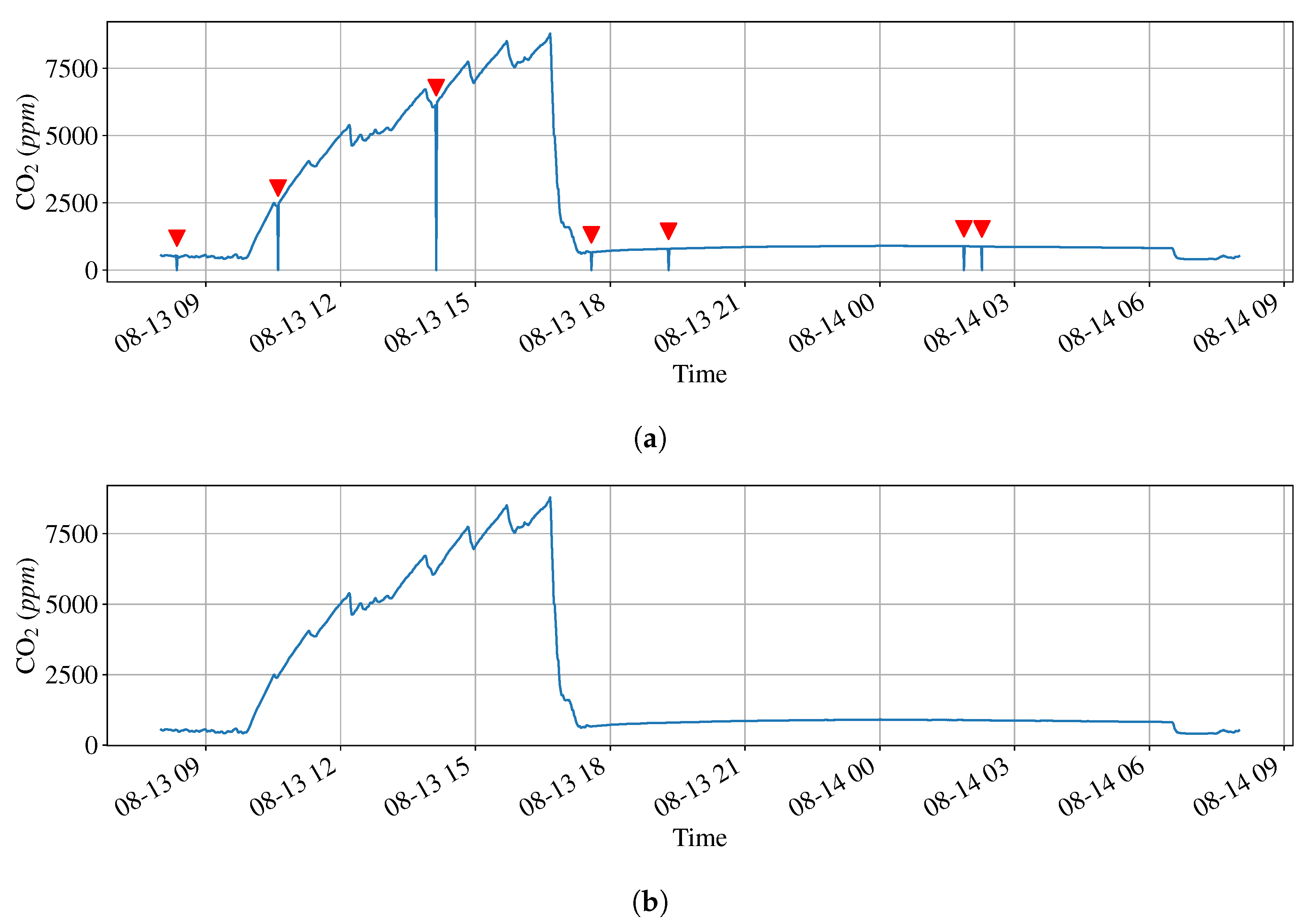
2.3. Data and Preprocessing

The data for this paper were collected through the airbox called MAPSv6, which uses Raspberry Pi [30] as the motherboard and ATMEGA2560 as the micro-controller unit (MCU) with several sensors. Several sensors installed on MAPSv6 include temperature, relative humidity, particulate matter (PM), luminosity, volatile organic compounds (VOCs), and carbon dioxide (CO₂). The brand and models are shown in

Table 1. Sensors on MAPSv6.

Sensing	Brand	Model	Units
Temperature (Temp)	Sensirion	STH31	°C
Relative humidity (RH)	Sensirion	STH31	%RH
Carbon dioxide (CO2)	SenseAir	S8	ppm
Volatile organic compounds (VOCs)	SenseAir	SGP30	ppb
Particulate matter (PM)	Plantower	PMS3003	μg/m3
Luminosity	Sunrom	TCS34725	Lux

.

Temperature and relative humidity have a strong correlation with the operation of air conditioning. Indoor particulate matter is less likely to fluctuate violently without combustion. The luminosity sensor is highly affected by indoor lighting. VOCs mostly evaporate from painting and coatings. Thus, we chose CO₂ as an indicator of indoor air quality that can reflect human activity which accumulated with time.

Figure 4 is the CO₂ concentrations data collected by an airbox device. The data collected from MAPSv6 have sensing errors or missing values. For example, in Figure 4a, there are seven errors or missing values. Hence, the first step was to remove the error value. The result of the example is shown in Figure 4b.

This paper uses the week as the unit of the data segment, since most people have a weekly cycle routine. In normal conditions, MAPSv6 senses every minute, so there will be 10,080 (60 (data/hour) × 24 (hours/day) × 7 (day/week)) data per week. Figure 5 shows an example of weekly CO₂ concentration.

However, due to the sensor anomaly and power instability, the amount of data collected may differ from the expected amount. The missing rate is the percentage of unusable data and the equation is defined in Equation (1). The number of collected data is the amount of data that removes the sensing error. The number of expected data collected is 10,080 in this case.

$$\mathrm{missing}\mathrm{rate}(\%)=\left(1-\frac{\mathrm{number}\mathrm{of}\mathrm{collected}\mathrm{data}}{\mathrm{number}\mathrm{of}\mathrm{expected}\mathrm{collected}\mathrm{data}}\right)\times 100\%$$

(1)

This paper uses a 10% missing rate as the threshold for similarity calculation for data accuracy. If the weekly data missing rate exceeds 10%, it will be discarded. Figure 6 shows the cumulative number of missing data for one data set. The red dashed horizon line is the 10% threshold, in which the data sets are only retained below the red dashed line, which results in the data of 764 devices per week.

The data sets are reaveraged in five-minute intervals after removing abnormal values and discarding data sets with excessive missing rates to compensate for missing values for short periods and correct for short-time offsets.

2.4. Methods

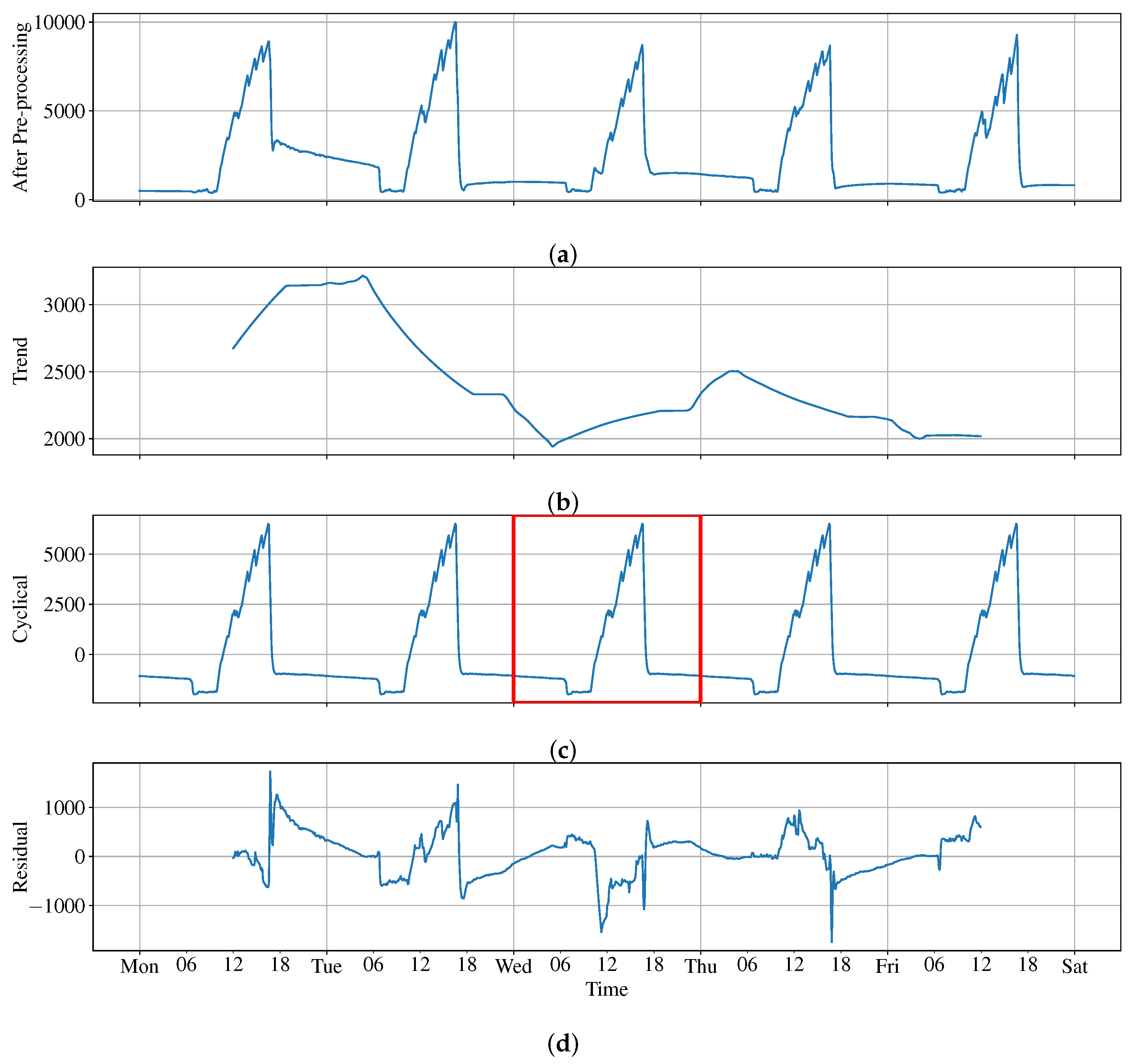
2.4.1. Time Series Decomposition

Time series data are a collection of observations arranged in time order, e.g., stock trend, daily temperatures, and sunspot numbers. In this paper, time series data (D) are defined in Equation (2), where n observation data, in which $d_i$ indicates the value at the time i.

$$D=(d_1,d_2,...,d_n)$$

(2)

Time series decomposition helps separate latent component sequences, especially for finding cyclical data [31]. Time series decomposition decomposes the original time series data into several components. Typical components include trend (T), cyclical (C), seasonal (S), and random (R). Different components are defined as follow:

• For trend (T), the trend component $t_i$ at the time i represents the general direction of change with the original data.
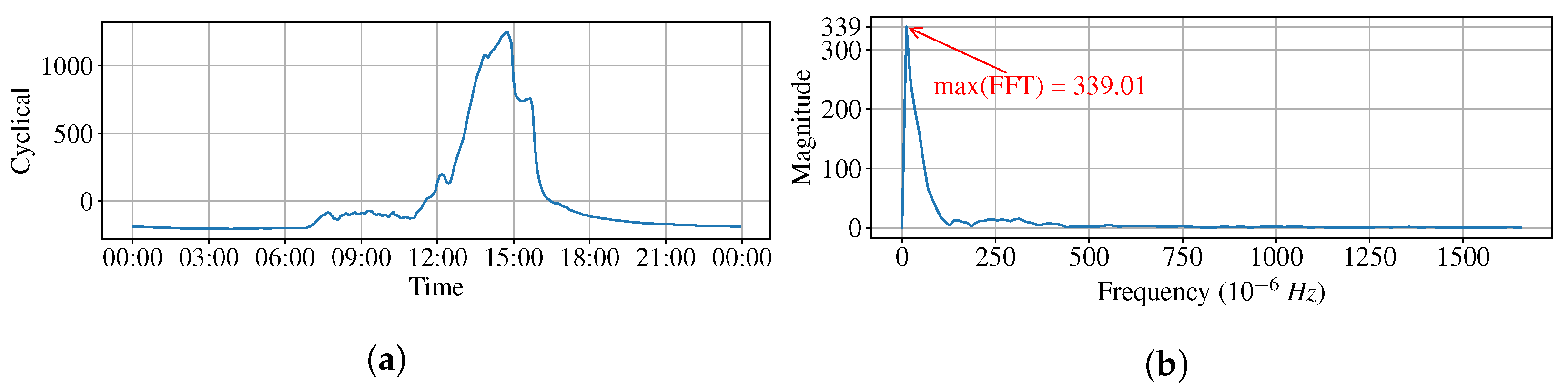
• For cyclical (C), the cyclical component $c_i$ at the time i indicates the repeated but nonperiodic fluctuations.
• For seasonal (S), the seasonal component $s_i$ at the time i denotes the repeating ups and downs of the seasons.
• For random (R), the random component $r_i$ at the time i is also known as residual or noise, and represents data that do not belong to previous components.

The original time series data can be recovered by combining the components. The raw data $d_i$ at the time i which can be obtained by summing or multiplying are defined in Equations (3) and (4), respectively, and the remaining components as defined previously.

$$d_i=t_i+c_i+s_i+r_i$$

(3)

$$d_i=t_i\times c_i\times s_i\times r_i$$

(4)

When the overall trend does not change significantly, it is more appropriate to use the additive model. In contrast, the multiplicative model is suitable when the trend changes drastically.

In this paper, the original data (i.e., preprocessed data) are decomposed into trends, periodicity, and residuals. First, a convolution filter is applied to the original data to obtain the trend data by the slide window average of the original data in the specific period. Second, the cyclical data are the average of each periodic interval of the removed trend data. Finally, the residual data are obtained by removing the trend and periodicity data from the original data. Figure 7 shows the flow chart of the decomposition process.

Figure 8 is an example of time series decomposition for CO₂ concentrations data. The original data (Figure 8a) is decomposed into several components called a trend (Figure 8b), cyclical (Figure 8c), and residual (Figure 8d). The frequency set for decomposition into one day is consistent with most space usage cycles. The cyclical component is repeated daily over the five days of data, which showed five identical fluctuations in Figure 8c. A single day data fragment, the red box in Figure 8c, is selected for closer examination in Figure 9.

In Figure 9, the red dashed line is the fluctuation after preprocessing and the solid blue line is the cyclical component after time series decomposition. The value of cyclical components is not the same as the original one. However, the fluctuation is highly correlated with the original trend.

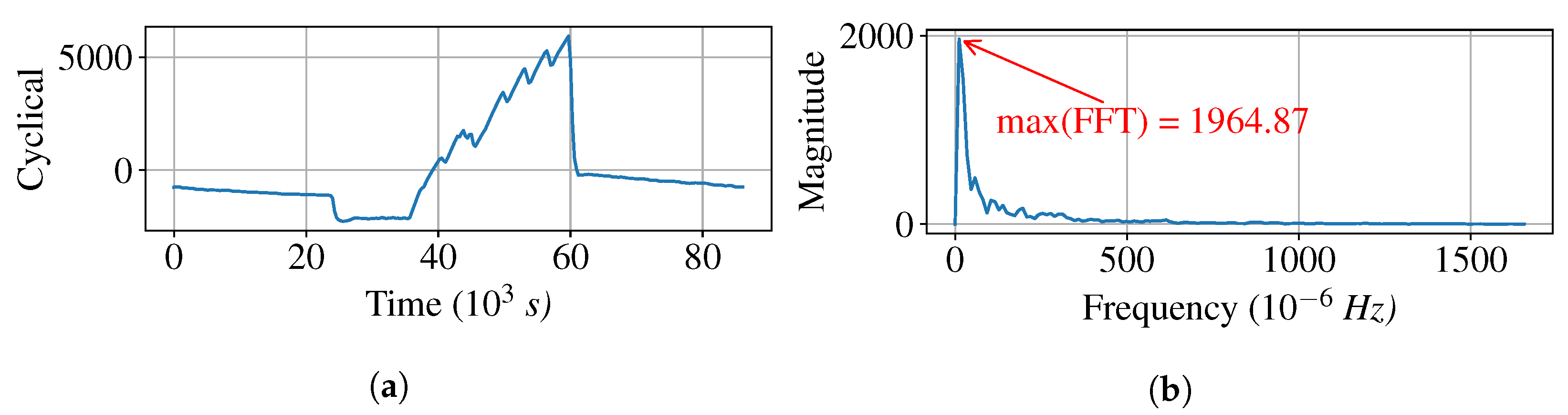
2.4.2. Fast Fourier Transform

Before discussing the fast Fourier transform (FFT) [32] used in this paper, we first introduce the discrete Fourier transform (DFT) [33]. Mathematically, a DFT is a linear integration transformation that converts the sequence (defined in Equation (5), where t is time) from a time domain (Figure 10a) into a frequency domain (Figure 10b). Both domains can be used for data analysis, and the frequency domain can represent the frequency information in the time domain.

$$\sum _{n=1}^{5}ncos\left(n\omega t\right),\omega =10\times 2\pi$$

(5)

The DFT is defined by Equation (6) from [34]. It transforms a sequence of N complex numbers $\left\{{\mathbf{x}}_n\right\}:=x_0,x_1,\dots ,x_{N-1}$ into another sequence of complex numbers, $\left\{{\mathbf{X}}_k\right\}:=X_0,X_1,\dots ,X_{N-1}$.

$$X_k=\sum _{n=0}^{N-1}{x}_n·e^{{\displaystyle -\frac{i2\pi }{N}kn}}$$

(6)

FFT is an algorithm used to calculate DFT. The time complexity of data size N of DFT is $O\left(N^2\right)$, but FFT is $O(NlogN)$, which can speed up the computation when the amount of data is enormous. Both DFT and FFT are linear transformations that can convert frequency domain data back to time domain data.

With the slightly stable CO₂ concentration data after preprocessing in Section 2.3 and time series decomposition in Section 2.4.1, the fluctuation of the data over time can be observed (Figure 11a). However, there may be hidden cyclical patterns in the data. For this reason, we use the FFT to convert the data from the time domain to the frequency domain (Figure 11b).

After transforming the CO₂ concentration data by the FFT, CO₂ data are expressed in the frequency domain. The maximum value of each frequency is selected as the indicator. The indicator of the CO₂ concentration, which is called max(FFT), is defined in Equation (7), where $\left\{{\mathit{X}}_k\right\}:=X_0,X_1,\dots ,X_{N-1}$ is the frequency domain sequence.

$$\begin{array}{cc}\hfill \max \left(\mathrm{FFT}\right)& =max\left\{{\mathit{X}}_k\right\}\hfill \\ \hfill & =max\left\{X_0,X_1,\dots ,X_{N-1}\right\}\hfill \end{array}$$

(7)

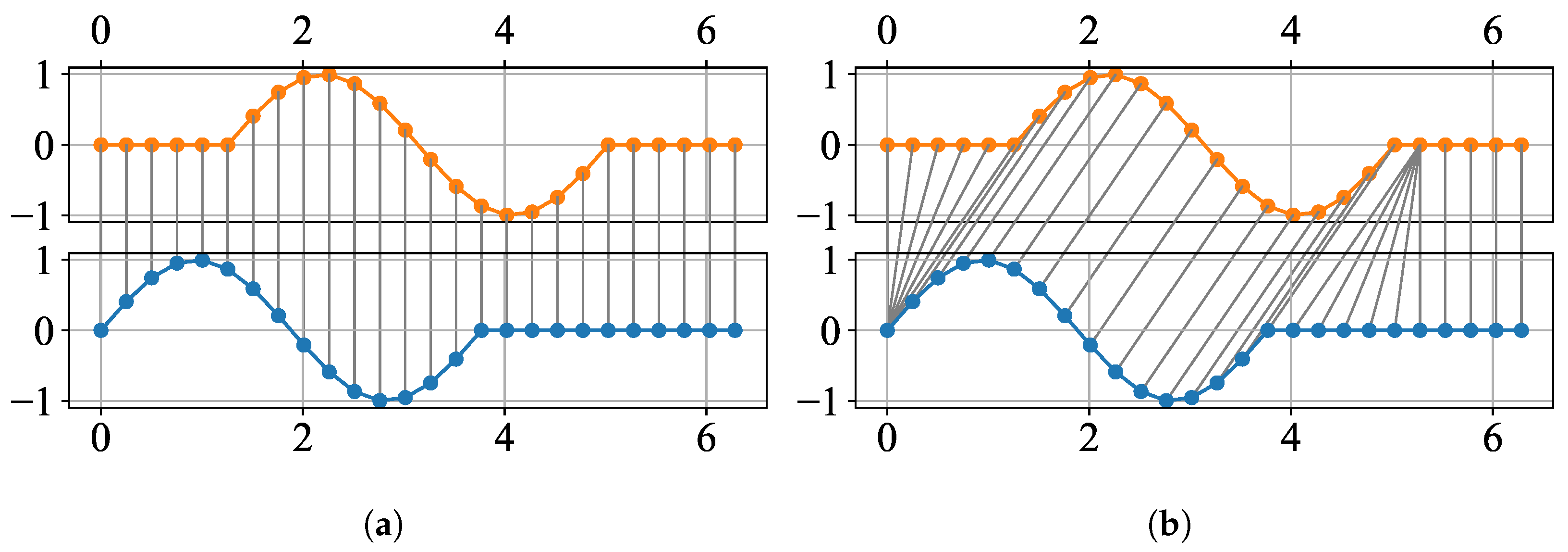
2.4.3. Dynamic Time Warping

For clustering time series data, we need to calculate the similarity for the data. The most common technique for comparing the similarity of two data points is using the Euclidean distance between two data points. However, Euclidean distance cannot calculate similarity when two time series data have different lengths. Another method to evaluate the similarity between time series data is called dynamic time warping (DTW) [34]. DTW can handle not only different sizes of data, but also deformations or shifts. Figure 12 visualize how the Euclidean distance and the dynamic time warping work.

In DTW, X and Y are two time series data sets which have m and n elements, where $X=\{x_1,x_2,...,x_m\}$ and $Y=\{y_1,y_2,...,y_n\}$. To dynamically calculate the minimum value of similarity (distance) between two data sets, we need to create a local cost matrix (LCM). The size of LCM (Figure 13) is $m\times n$ and the element at position $(i,j)$ is the distance between $x_i$ and $y_j$. The LCM in q-dimensional space is shown as Equation (8) from [34].

$$lcm(i,j)={\left(\sum _{i=0}^{m-1}\sum _{j=0}^{n-1}{\left(x_i-y_j\right)}^q\right)}^{\frac{1}{q}}$$

(8)

With LCM, two time series data are aligned. We find a path $\pi$ (upper-right red line in Figure 13) of length $max(m,n)$ from $lcm(0,0)$ to $lcm(m,n)$, which represents the minimum distance between two time series data. Thus, the DTW for X and Y is calculated with Equation (9) from [34], where $d(x_i,y_j)$ means the distance between $x_i$ and $y_j$, and $\mathcal{A}(X,Y)$ indicates the set of all admissible paths.

$$DT{W}_q(X,Y)=\underset{\pi \in \mathcal{A}(X,Y)}{min}{\left(\sum _{(i,j)\in \pi }d{(x_i,y_j)}^q\right)}^{\frac{1}{q}}$$

(9)

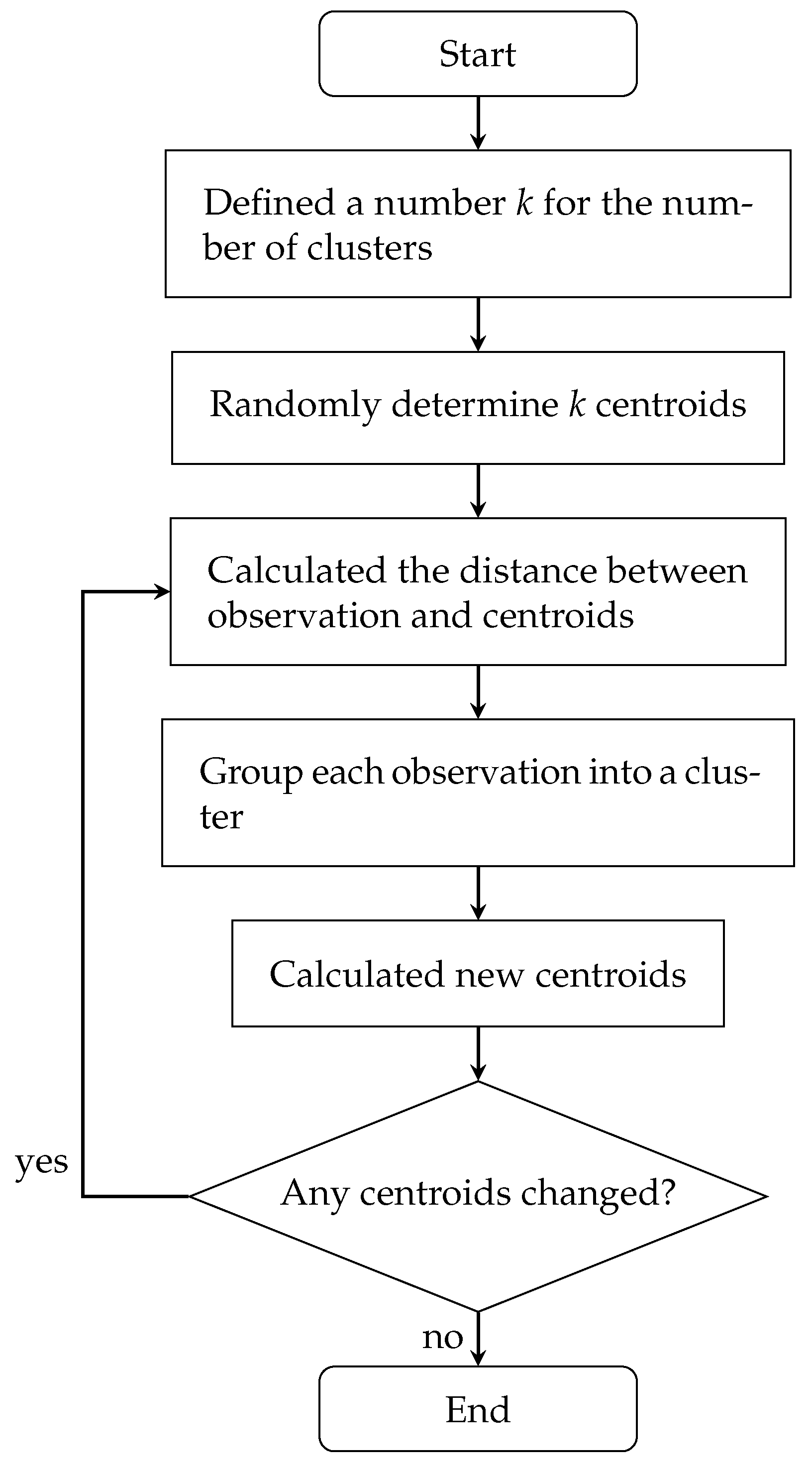
2.4.4. K-Means Clustering

In unsupervised clustering, prelabeling of the data is not required to classify with unknown field types. K-means clustering is one kind of asymptotic unsupervised algorithm which can converge the result with several iterations. K-means aims to cluster n observations into k clusters, in which k is a predefined number. K-means clustering has been used in various studies [35], which can cluster not only one-dimensional data [8,9,10] but also time series data [17]. Figure 14 is the flow chart of K-means clustering with the following steps:

• Define a number k for the number of clusters.
• Randomly determine k centroids.
• Calculate the distance between observation data point and centroids.
• Group each observation into a cluster.
• Calculate new centroids.
• Go to the next step if all centroids are unchanged; otherwise, go to step 3
• End of clustering.

Figure 14. K-means clustering flow chart.

Figure 14. K-means clustering flow chart.

There are three indicators for the CO₂ concentration cyclical component: the original data of weekly CO₂ concentration, one-day segment time series data, and max(FFT). To classify the field types, each indicator needs to be clustered into a category. However, they use different methods to evaluate their similarity. The time series data may have characteristics such as varying length or offsets. In this paper, DTW is used to measure the similarity between the time series data to overcome the issues. The max (FFT) treated as one-dimensional clustering used Euclidean distance for similarity measurement.

3. Results and Discussion

This section introduces all experiments performed in this research. The experiment environment used for this research had an AMD Ryzen 7 3700X 8-Core Processor CPU, 16 GB × 2 RAM, and Ubuntu 18.04.4 LTS as the operating system. The Python version was 3.6.9. First, a cluster was used with raw CO₂ concentration data. After decomposing, the cyclical component was used as clustering data. Third, FFT was used to transfer the CO₂ concentration cyclical component from a time domain to a frequency domain. Then, the max(FFT) was applied for clustering.

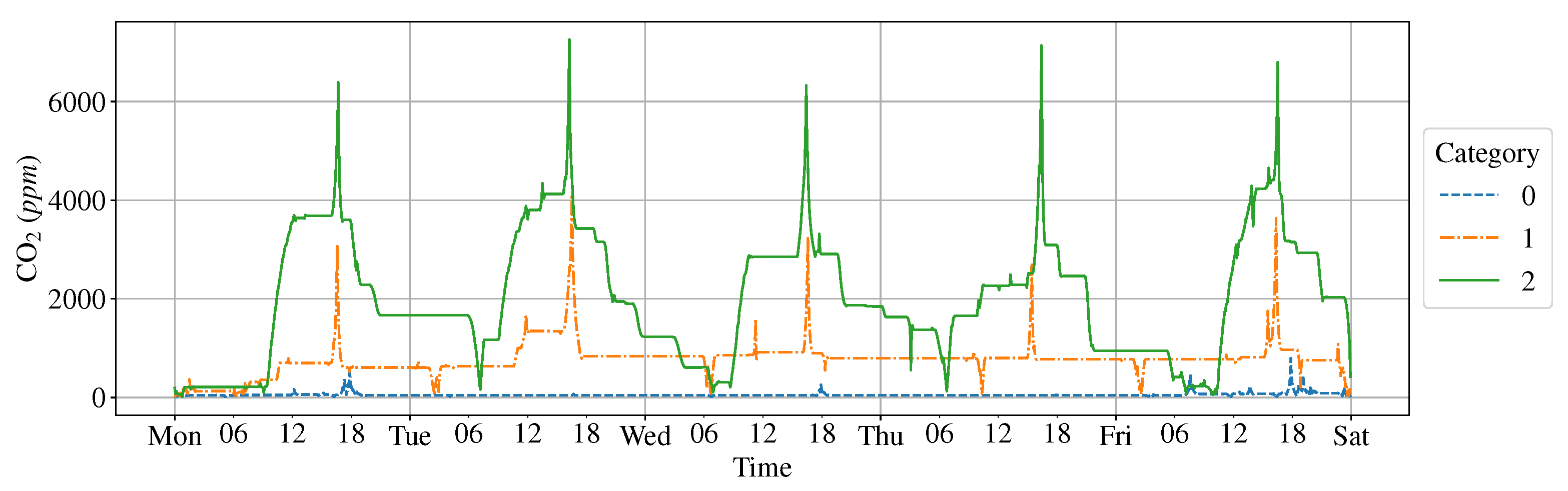
3.1. Cluster Result with Raw Data

We used the data set collected from the junior high school campus mentioned in Section 2.1. The background values were removed before using the raw data for clustering. In this paper, the minimum value of CO₂ concentration for that week was used as the background value. It was clustered with K-means and DTW was utilized as a distance measurement method. The number of devices per week data clustered into three categories; see Figure 15. All 764 devices per week data were clustered into three categories, such as 710 devices per week in Category 0, 38 devices per week in Category 1, and 16 devices per week in Category 2.

Figure 16 shows the centroid of the raw data clustering results after ten iterations on the K-means clustering algorithm. There are three lines representing each category’s centroids. The solid green line represents the centroid of the field with the highest CO₂ concentration. The orange dash–dotted line denotes the field with the middle level of CO₂ concentration centroid. The lowest blue dashed line is the centroid of the field with the lower CO₂ concentration.

In Figure 17, we compared six different devices from different weeks and categories, randomly choosing two devices per week from each category. For example, “7E2EF7, W10, C0” represents week 10 of device id 7E2EF7 clustered to Category 0. As in Figure 16, the solid line indicates the field with the highest concentration. The dash–dotted lines are the next highest, and the dashed lines are the field with the lowest concentration. There is a significant distinction between the three categories, which indicates that the classification method has good results.

Figure 18 is the heat map showing the clustering results. The x-axis is the week count, counting from the first-week devices available, and the y-axis represents the devices mounted on different fields. The color shade represents the device per week cluster in each category. All of the devices per week clustering in Category 2 are at the beginning of data collection. Category 1 is distributed at all times. The devices per week in Category 0 represented in the field did not accumulate too much CO₂ in the indoor environment.

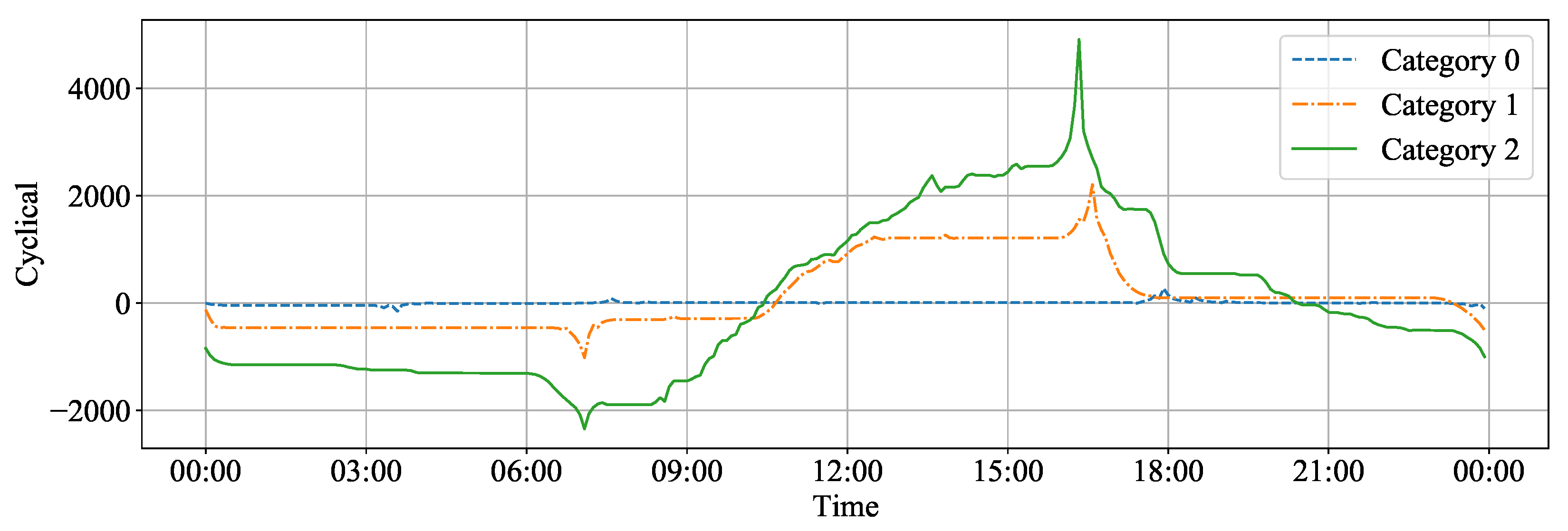
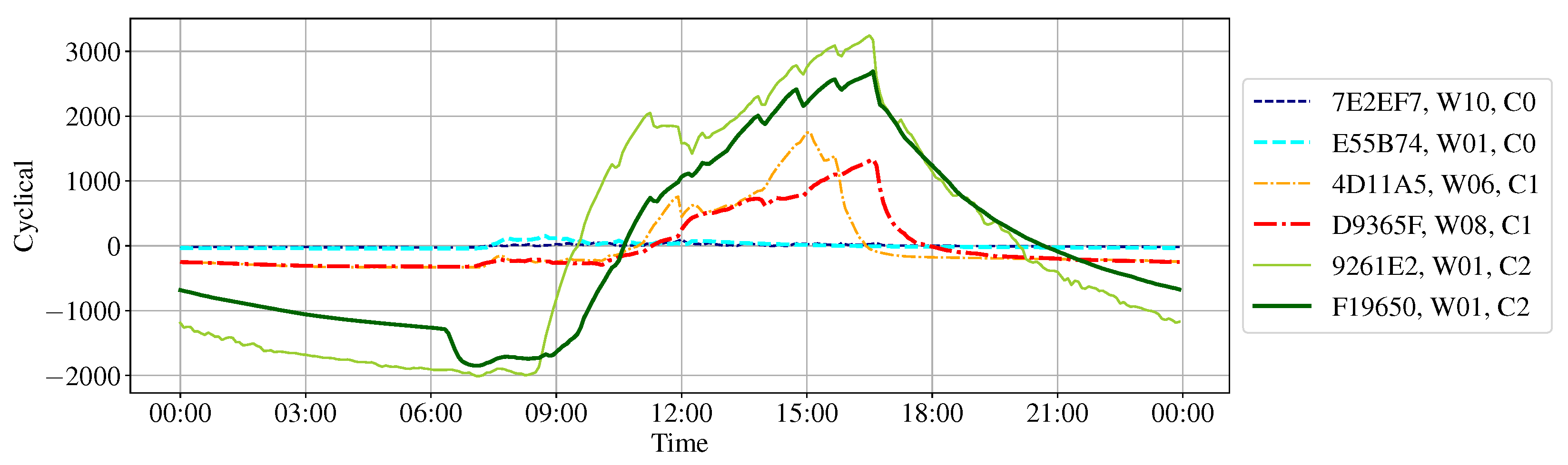
3.2. Cluster Result with Cyclical Components

The data set used in this experiment is the same as in Section 3.1. A total of 764 devices per week were used to cluster. Before clustering, the time series data were decomposed into trend, cyclical, and residual components. The cyclical components revealed the daily repeated fluctuation in the week which was used for clustering in this section. Since the cyclical components repeated daily, we were able to reduce the data to a single day segment to represent the devices’ daily data. Reducing the number of every device per week series data from 1440 (5 days × 24 hours/day × 12 data/hour) in the Section 3.1 to 288 (24 hours/day × 12 data/hour) could reduce the calculation time.

The cyclic component of one-day segments were clustered using the K-means algorithm with the DTW measure similarity. Figure 19 shows the number of devices per week clustering into each category. There are 722 devices per week belonging to Category 0, 30 devices per week in Category 1, and 12 devices per week in Category 2. Compared with Figure 15, there were fewer devices per week clustered in categories 1 and 2 in Figure 19.

The centroid of each category is shown in Figure 20. As in Figure 16, the lines in Figure 20 each represent a category: dashed for Category 0, dash–dotted for Category 1, and solid lines for Category 2. Categories 1 and 2 have the lowest level of the entire segment at 7:00 am. The reason is that windows and doors were opened for classroom preparation. As for Category 0, the fluctuation is flatter than in the two other categories. There is a rising trend in all categories around 7:30 am to 8:00 am caused by occupants (i.e., students and teachers) starting to use the space. All categories’ cyclical components reach their maximum circulation between 16:00 and 18:00, which is the cumulative result of the day’s usage. There is a decreasing trend in all categories after cyclical components reach the maximum.

In Figure 21, we compared six different devices from different weeks and categories that are similar to Figure 17’s two devices per week from each category. Two dashed lines represent the device per week cluster into Category 0. There is less fluctuation compared to the other two categories, but there is still a slight fluctuation between 7:00 and 9:00 am due to the starting of classes. The device per week represents two solid lines belonging to Category 2, which has the highest CO₂ concentration cyclical components. The device per week data that clustered to Category 2 indicates the field has poor ventilation on that week. There is a downward trend around 6:00 am in the cyclical component of device F19650 on week 1. The dash–dotted devices per week are clustered in Category 1. In Category 1, CO₂ concentration cyclical components are not as high as in Category 2, but they are not as flat as in Category 0.

Figure 22 shows the heat map of the clustering result on each device per week. Compared with Figure 18, four devices were classified as Category 2 in the previous result and became Category 1, and twelve devices were clustered as Category 1 in the previous result and became Category 0 with cyclical components clustering.

In Figure 23, four devices per week selected for this result differ from the previous result. Two of them are changed from Category 1 to Category 0, and two others are from Category 2 to Category 1. The device per week’s category from 1 to 0 represented in dash–dotted lines are week 36 of the device F19650 and week 12 of the device 753B56. Both of them only have one-day fluctuation during the five-day segment, which has no repetition fluctuation in cyclical components. The devices per week in solid lines week 7 of the device 9261E2 and week 7 of the device AE9F98 are changed from Category 2 to Category 1. Their lowest level in the cyclical component is higher than the devices classified in Category 2 in both cluster results due to the insufficient CO₂ concentration drops at am 7:00 in their original data repetition.

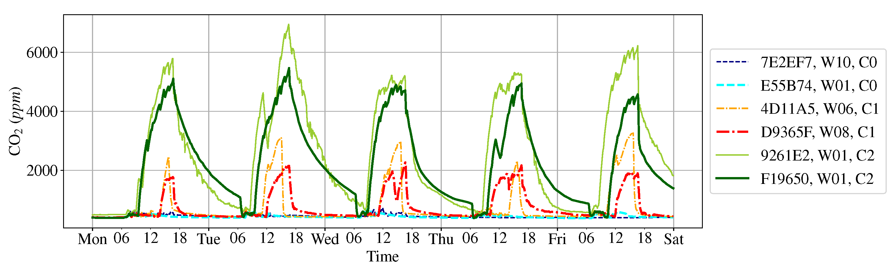
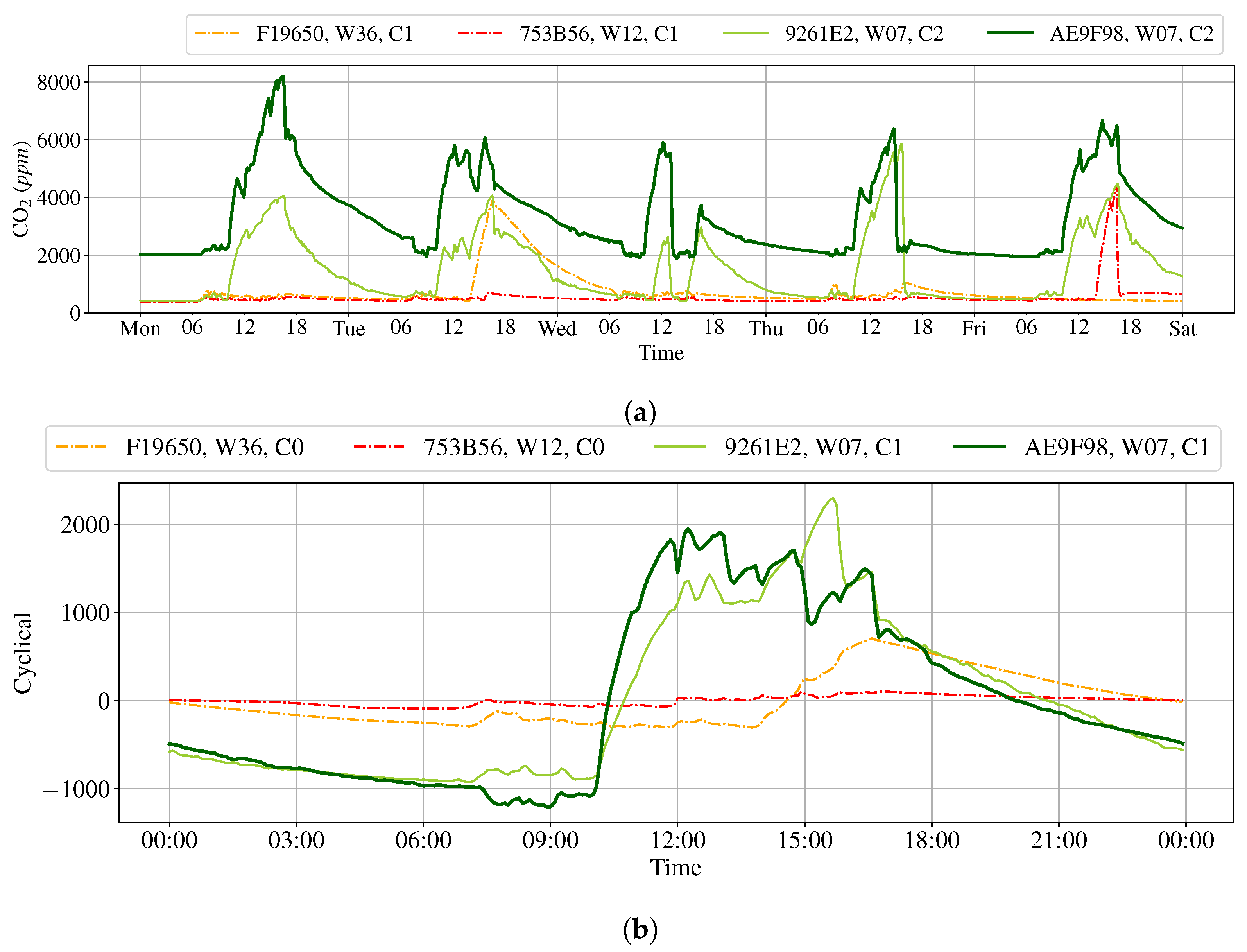
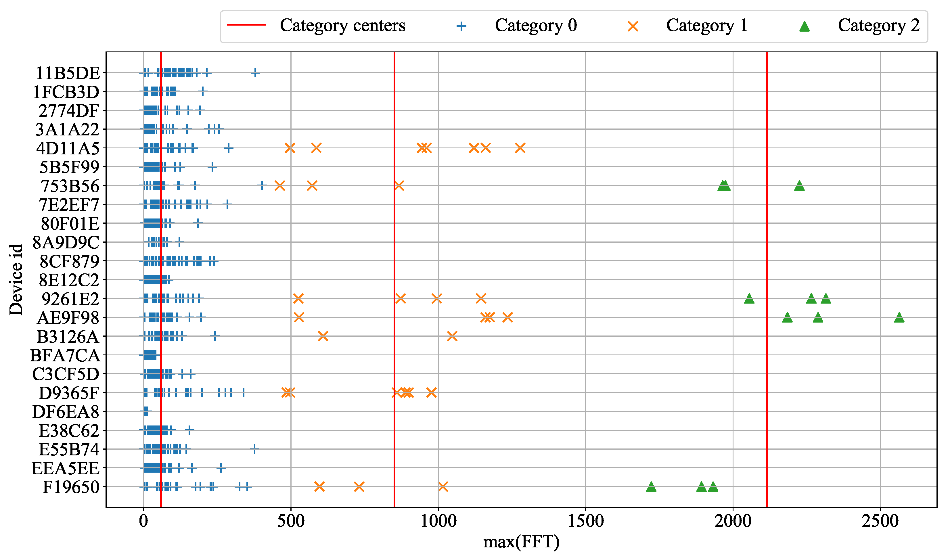
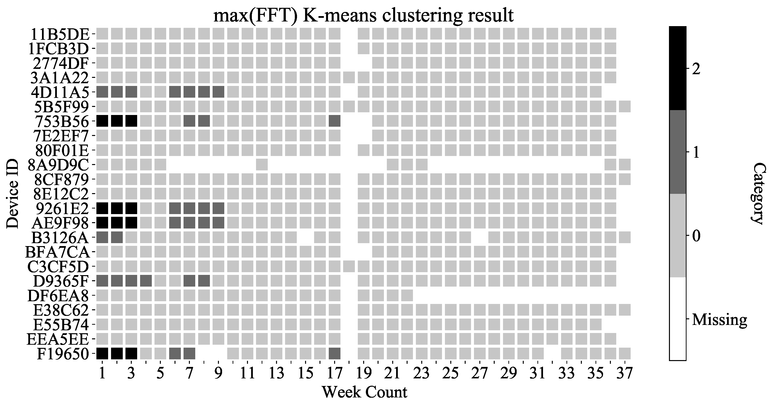
3.3. Cluster Result with Max (FFT)

In this experiment, the fast Fourier transform (FFT) is used to transfer cyclical components from a time domain into a frequency domain. Then, the maximum in the frequency domain sequence is selected as max (FFT) as an indicator of device per week, as described in Section 2.4.2. The number of devices per week clusters into three categories; see Figure 24. Twelve devices per week are clustered in Category 2, 29 devices per week cluster in Category 1, and the rest are in Category 0. Only one change from the previous cluster result is a device per week change from Category 1 to Category 0, compared with Figure 19.

The max (FFT) cluster centers are shown in Figure 25. The “plus” symbol is a device per week in Category 0, the “cross” symbol represents a device per week in Category 1, and the “triangle” symbol is a device per week in Category 2. Three red lines are arithmetic, which means that they indicate the categories’ center. Each device per week’s max(FFT) is clustered into a category, which has a closer distance to the centers than other categories.

Figure 26 represents the results of max(FFT) cluster in a heat map. There is only one difference from the previous cluster result (see Figure 22) in week 6 of the device D9365F, of which the cyclical component is shown in Figure 27.

Figure 27a showed that the time domain of the concentration trend for the device D9365F increased near noon and decreased significantly at 15:00. The event produced steeper inclines and declined slopes compared with other devices per week. After FFT, the wave transformed to a smaller maximum amplitude in the frequency domain (see Figure 27b) than the other devices per week. As a result, the device D9365F’s data for week 6 clustered into a different category compared wit the previous clustering technique.

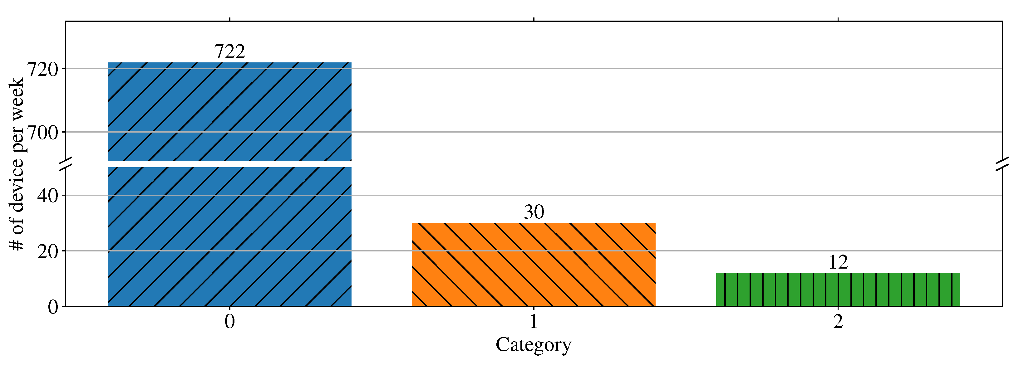
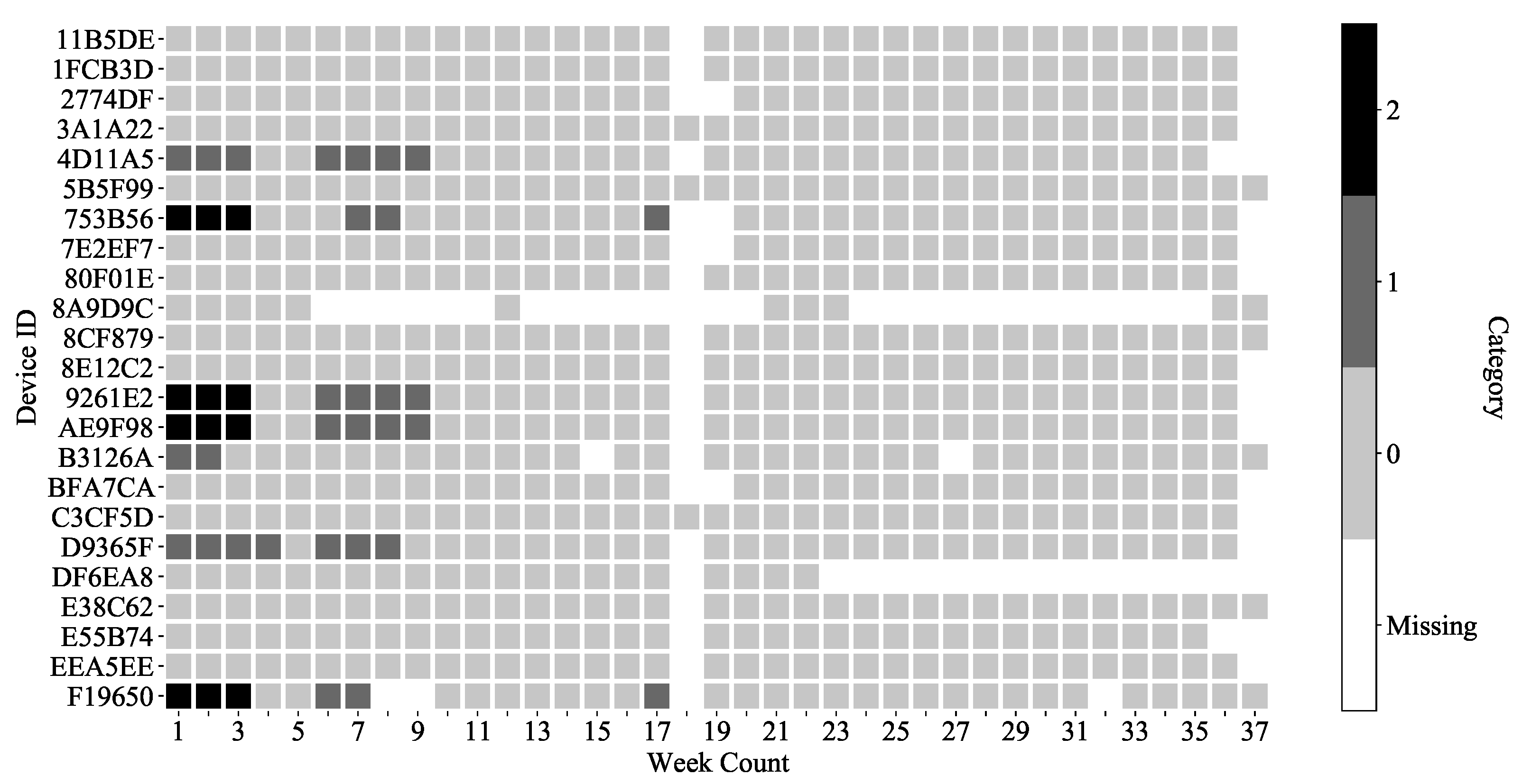
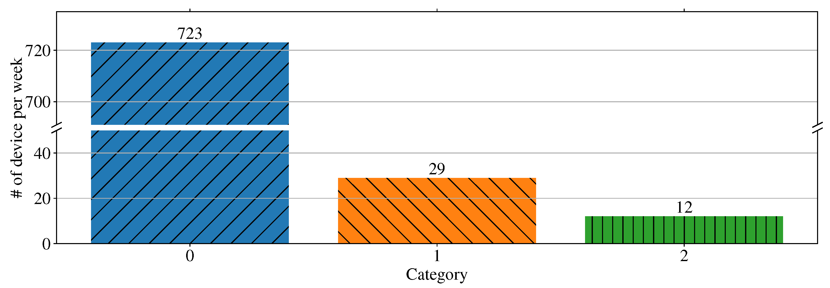
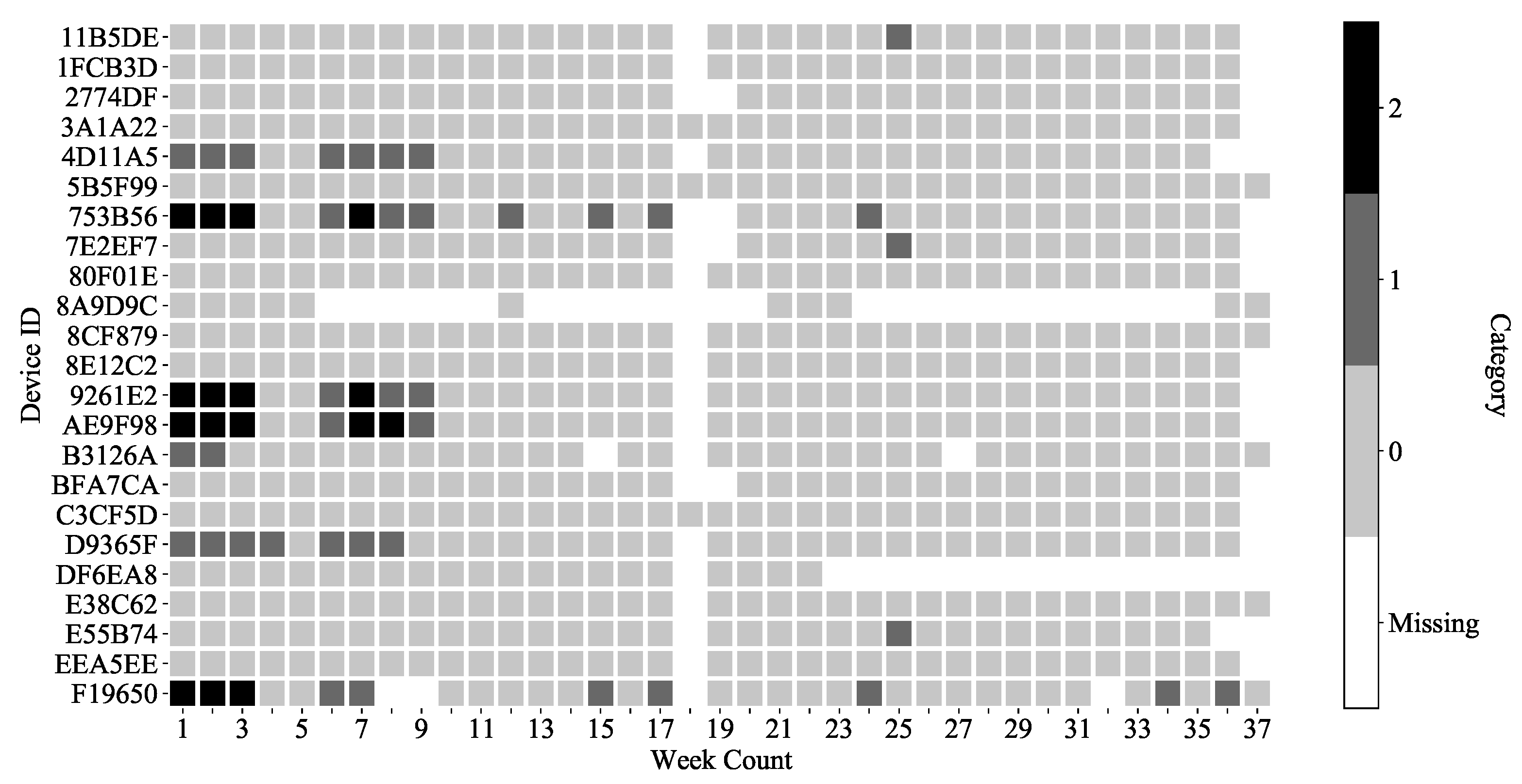
3.4. Type Definition on K-Means Clustering Result

The three clustering methods are based on the devices per week. However, this causes the same space (e.g., classroom) to be clustered into several different categories. Devices belonging to several different categories will lead to difficulties in further analysis and utilization. Therefore, it is necessary to define rules to transfer the previously mentioned clustering categories to types.

To simplify the process, we classify 22 devices into three types based on the K-means clustering result, as follows:

• Type 2 is devices with any weekly data classified as Category 2.
• Type 1 is devices with any weekly data classified as Category 1.
• Type 0 is the remaining devices.

Figure 28 is the school map with three types of cluster. Only four devices belong to Type 2, with device IDs 753B56, 9261E2, AE9F98, and F19650. All devices that cluster to Type 2 are installed in the classrooms equipped with air conditioners by the southwest campus. They are the fields that need the most improvement to reduce indoor CO₂ concentration. The devices with ID 4D11A5 and D9365F belong to Type 1. Both of them are on the south side of the campus and also have air conditioning. In the case of devices belonging to Type 0, the accumulation of CO₂ in the field is not as intense as in type 1 and 2.

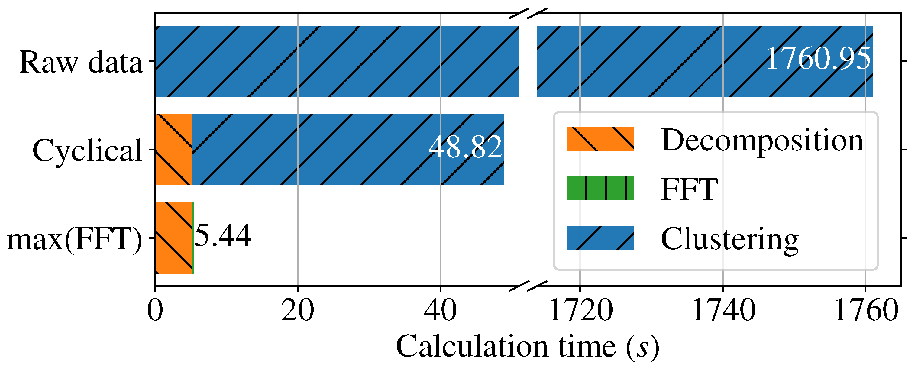
3.5. Calculation Time

In this section, we will compare the total calculation time for three clustering techniques. The total calculation time for clustering process includes the clustering time, time series decomposition time, and the time for fast Fourier transformations. Each clustering technique is shown in

Table 2. Calculation time.

Calculation Time (in s)	Decomposition	FFT	Clustering	Total
Raw	N/A	N/A	1760.95	1760.95
Cyclical	5.221	N/A	43.596	48.817
max(FFT)	5.221	0.194	0.025	5.444

and Figure 29.

Raw data clustering is mentioned in Section 3.1 which takes almost half an hour (1760 s) to cluster. Calculation time for cyclical components clustering (Section 3.2) consists of decomposition and clustering time. The time for decomposition takes 5.2 s. However, the clustering time is reduced to 43 s. Therefore, the total calculation time for cyclical component clustering is 48 s. The proposed fast Fourier transfer required for max(FFT) clustering (Section 3.3) takes 0.1 s to convert all the data from a time domain to a frequency domain. The clustering takes 0.025 s. This makes the proposed fast Fourier transfer max(FFT) clustering approach the one with the lowest total calculation time: 5.4 s.

4. Conclusions

In this paper, we proposed a clustering method called Max Fast Fourier Transform (maxFFT) to cluster indoor air quality without using any additional information, e.g., environmental conditions, location, or the number of people. MaxFFT clustering comprised several steps, including preprocessing, time series decomposing, fast Fourier transfer, and K-means clustering. For our experiments, the real-world data set was collected from a junior high school campus for 261 days.

We compared experimental results of the proposed maxFFT with the observed conditions from the actual field trials. Results showed that maxFFT correctly reflected actual field conditions such as indoor air quality, locations, time, and usage of different classrooms. Compared with raw data clustering and cyclical components clustering, maxFFT is able to achieve more actual cluster results while using the lowest computing time. According to our experiment results, the maxFFT clustering method required significantly lower computation time. The computation times required for different clustering approaches are important for big data sets.

Although the time series decomposition strategy and fast Fourier transformation can cluster the observed data, it still has its limitations when it comes to tackling the trend. In the future, different decomposition methods or transformation methods can be considered. In this study, we only used CO₂ as an indicator for indoor air quality for clustering. For future work, more variables can be used as indoor air-quality indicators collected by the other sensors on MAPSv6 to represent indoor air quality.

In terms of temporal resolution, we used one week as the time unit for clustering, since most people repeat their routine weekly. Other temporal resolutions can be considered for further clusterings, such as a month or season. Once we have an accurate indoor air-quality cluster, the results can be used to predict future air quality or implement policies for air-quality improvements.

References

1. WHO. Air Pollution. 2016. Available online: https://www.who.int/health-topics/air-pollution (accessed on 20 July 2022).
2. Mahyuddin, N.; Awbi, H. A Review of CO2 Measurement Procedures in Ventilation Research. Int. J. Vent. 2012, 10, 353–370. [Google Scholar] [CrossRef]
3. U.S. EPA. Indoor Air Quality (IAQ). Available online: https://www.epa.gov/indoor-air-quality-iaq (accessed on 20 July 2022).
4. Jones, A. Indoor air quality and health. Atmos. Environ. 1999, 33, 4535–4564. [Google Scholar] [CrossRef]
5. Bramer, M. Clustering; Springer: Berlin/Heidelberg, Germany, 2007. [Google Scholar]
6. Danielsson, P.E. Euclidean distance mapping. Comput. Graph. Image Process. 1980, 14, 227–248. [Google Scholar] [CrossRef]
7. Fisher, R.A. The use of multiple measurements in taxonomic problems. Ann. Eugen. 1936, 7, 179–188. [Google Scholar] [CrossRef]
8. Chakraborty, A.; Faujdar, N.; Punhani, A.; Saraswat, S. Comparative Study of K-Means Clustering Using Iris Data Set for Various Distances. In Proceedings of the 2020 10th International Conference on Cloud Computing, Data Science Engineering (Confluence), Noida, India, 29–31 January 2020; pp. 332–335. [Google Scholar] [CrossRef]
9. Caron, A.; Redon, N.; Coddeville, P.; Hanoune, B. Identification of indoor air quality events using a K-means clustering analysis of gas sensors data. Sens. Actuators B Chem. 2019, 297, 126709. [Google Scholar] [CrossRef]
10. Sunori, S.K.; Negi, P.B.; Maurya, S.; Juneja, P.; Rana, A. K-Means Clustering of Ambient Air Quality Data of Uttarakhand, India during Lockdown Period of COVID-19 Pandemic. In Proceedings of the 2021 6th International Conference on Inventive Computation Technologies (ICICT), Coimbatore, India, 20–22 January 2021; pp. 1254–1259. [Google Scholar]
11. Chen, Y.; Wang, L.; Li, F.; Du, B.; Choo, K.K.R.; Hassan, H.; Qin, W. Air quality data clustering using EPLS method. Inf. Fusion 2017, 36, 225–232. [Google Scholar] [CrossRef]
12. Zhu, C.; Li, N. Study on grey clustering model of indoor air quality indicators. Procedia Eng. 2017, 205, 2815–2822. [Google Scholar] [CrossRef]
13. Delgado, A.; Montellanos, P.; Llave, J. Air quality level assessment in Lima city using the grey clustering method. In Proceedings of the 2018 IEEE International Conference on Automation/XXIII Congress of the Chilean Association of Automatic Control (ICA-ACCA), Concepcion, Chile, 17–19 October 2018; pp. 1–4. [Google Scholar] [CrossRef]
14. Chang, J.H.; Tseng, C.Y.; Chiang, H.H.; Hwang, R.H. Analysis of Influential Factors in Secondary PM2.5 by K-Medoids and Correlation Coefficient. In Proceedings of the 2017 IEEE 7th International Symposium on Cloud and Service Computing (SC2), Kanazawa, Japan, 22–25 November 2017; pp. 177–182. [Google Scholar]
15. Aghabozorgi, S.; Seyed Shirkhorshidi, A.; Ying Wah, T. time series clustering—A decade review. Inf. Syst. 2015, 53, 16–38. [Google Scholar] [CrossRef]
16. Dincer, N.G.; Akkuş, Ö. A new fuzzy time series model based on robust clustering for forecasting of air pollution. Ecol. Inform. 2018, 43, 157–164. [Google Scholar] [CrossRef]
17. Alahamade, W.; Lake, I.; Reeves, C.E.; De La Iglesia, B. A multi-variate time series clustering approach based on intermediate fusion: A case study in air pollution data imputation. Neurocomputing 2021, 490, 229–245. [Google Scholar] [CrossRef]
18. Li, J.; Izakian, H.; Pedrycz, W.; Jamal, I. Clustering-based anomaly detection in multivariate time series data. Appl. Soft Comput. 2021, 100, 106919. [Google Scholar] [CrossRef]
19. Samet, J.M.; Marbury, M.C.; Spengler, J.D. Health Effects and Sources of Indoor Air Pollution. Part I. Am. Rev. Respir. Dis. 1987, 136, 1486–1508. [Google Scholar] [CrossRef] [PubMed]
20. Abdullahi, K.L.; Delgado-Saborit, J.M.; Harrison, R.M. Emissions and indoor concentrations of particulate matter and its specific chemical components from cooking: A review. Atmos. Environ. 2013, 71, 260–294. [Google Scholar] [CrossRef]
21. Samet, J.M. Radon and Lung Cancer. JNCI J. Natl. Cancer Inst. 1989, 81, 745–758. [Google Scholar] [CrossRef]
22. Turanjanin, V.; Vučićević, B.; Jovanović, M.; Mirkov, N.; Lazović, I. Indoor CO2 measurements in Serbian schools and ventilation rate calculation. Energy 2014, 77, 290–296. [Google Scholar] [CrossRef]
23. Scheff, P.A.; Paulius, V.K.; Huang, S.W.; Conroy, L.M. Indoor Air Quality in a Middle School, Part I: Use of CO2 as a Tracer for Effective Ventilation. Appl. Occup. Environ. Hyg. 2000, 15, 824–834. [Google Scholar] [CrossRef]
24. Satish, U.; Mendell, M.J.; Shekhar, K.; Hotchi, T.; Sullivan, D.; Streufert, S.; Fisk, W.J. Is CO2 an Indoor Pollutant? Direct Effects of Low-to-Moderate CO2 Concentrations on Human Decision-Making Performance. Environ. Health Perspect. 2012, 120, 1671–1677. [Google Scholar] [CrossRef]
25. Azuma, K.; Kagi, N.; Yanagi, U.; Osawa, H. Effects of low-level inhalation exposure to carbon dioxide in indoor environments: A short review on human health and psychomotor performance. Environ. Int. 2018, 121, 51–56. [Google Scholar] [CrossRef]
26. Oneṭ, A.; Ilieș, D.C.; Ilieṣ, A.; Herman, G.V.; Burtă, L.; Marcu, F.; Buhaṣ, R.; Caciora, T.; Baias, Ṣ.; Oneṭ, C.; et al. Indoor air quality assessment and its perception. Case study–historic wooden church, Romania. Rom. Biotechnol. Lett. 2020, 25, 1547–1553. [Google Scholar] [CrossRef]
27. Ilieș, D.C.; Hodor, N.; Indrie, L.; Dejeu, P.; Ilieș, A.; Albu, A.; Caciora, T.; Ilieș, M.; Barbu-Tudoran, L.; Grama, V. Investigations of the Surface of Heritage Objects and Green Bioremediation: Case Study of Artefacts from Maramureş, Romania. Appl. Sci. 2021, 11, 6643. [Google Scholar] [CrossRef]
28. Chen, L.J.; Ho, Y.H.; Lee, H.C.; Wu, H.C.; Liu, H.M.; Hsieh, H.H.; Huang, Y.T.; Lung, S.C.C. An Open Framework for Participatory PM2.5 Monitoring in Smart Cities. IEEE Access 2017, 5, 14441–14454. [Google Scholar] [CrossRef]
29. Ho, Y.H.; Li, P.E.; Chen, L.J.; Liu, Y.L. Indoor Air Quality Monitoring System for Proactive Control of Respiratory Infectious Diseases: Poster Abstract. In Proceedings of the 18th Conference on Embedded Networked Sensor Systems, Virtual, 16–19 November 2020; Association for Computing Machinery: New York, NY, USA, 2020; pp. 693–694. [Google Scholar] [CrossRef]
30. Upton, E.; Halfacree, G. Raspberry Pi User Guide; John Wiley & Sons: Hoboken, NJ, USA, 2014. [Google Scholar]
31. WEST, M. Time series decomposition. Biometrika 1997, 84, 489–494. [Google Scholar] [CrossRef]
32. Heideman, M.T.; Johnson, D.H.; Burrus, C.S. Gauss and the history of the fast Fourier transform. Arch. Hist. Exact Sci. 1985, 34, 265–277. [Google Scholar] [CrossRef]
33. Winograd, S. On computing the discrete Fourier transform. Math. Comput. 1978, 32, 175–199. [Google Scholar] [CrossRef]
34. Dynamic Time Warping. In Information Retrieval for Music and Motion; Springer: Berlin/Heidelberg, Germany, 2007; pp. 69–84. [CrossRef]
35. Jain, A.K. Data clustering: 50 years beyond K-means. Pattern Recognit. Lett. 2010, 31, 651–666. [Google Scholar]
36. Location Aware Sensor System, LASS. 2016. Available online: https://lass-net.org/ (accessed on 20 July 2022).
Figure 1. Campus map.
Atmosphere 13 01375 g001
Figure 2. Data collection period.
Atmosphere 13 01375 g002
Figure 3. Experiment flow chart.
Atmosphere 13 01375 g003
Figure 4. Data preprocessing on CO2 concentration. (a) Raw data collected from air box. (b) Remove sensing error data.
Atmosphere 13 01375 g004
Figure 5. Weekly CO2 concentration.
Atmosphere 13 01375 g005
Figure 6. CO2 missing rate.
Atmosphere 13 01375 g006
Figure 7. Time series decomposition flow chart.
Atmosphere 13 01375 g007
Figure 8. CO2 concentration time series decomposition. (a) Original data; (b) trend component; (c) cyclical component; (d) residual component.
Atmosphere 13 01375 g008
Figure 9. Cyclical component 1 day segment.
Atmosphere 13 01375 g009
Figure 10. Different domain on the same wave. (a) Time domain; (b) Frequency domain.
Atmosphere 13 01375 g010
Figure 11. CO2 concentration cyclical component. (a) Time domain; (b) frequency domain.
Atmosphere 13 01375 g011
Figure 12. Different methods to evaluate the distance between two time series data. (a) Euclidean distance; (b) DTW alignment.
Atmosphere 13 01375 g012
Figure 13. Alignment on local cost matrix.
Atmosphere 13 01375 g013
Figure 15. Number of devices per week on different cluster.
Atmosphere 13 01375 g015
Figure 16. Centroid of raw CO2 concentration clustering.
Atmosphere 13 01375 g016
Figure 17. Raw data cluster result sample.
Atmosphere 13 01375 g017
Figure 18. Raw data clustering result with week count.
Atmosphere 13 01375 g018
Figure 19. Number of device per week on cyclical component clustering.
Atmosphere 13 01375 g019
Figure 20. Centroid of cyclical component clustering.
Atmosphere 13 01375 g020
Figure 21. Cyclical component cluster result sample.
Atmosphere 13 01375 g021
Figure 22. Cyclical components clustering result with week count.
Atmosphere 13 01375 g022
Figure 23. Results of different clustering techniques. (a) Raw data; (b) Cyclical components.
Atmosphere 13 01375 g023
Figure 24. Device per week count on max(FFT) K-means cluster result.
Atmosphere 13 01375 g024
Figure 25. Categories center of max(FFT) clustering result.
Atmosphere 13 01375 g025
Figure 26. max(FFT) clustering result with week count.
Atmosphere 13 01375 g026
Figure 27. Week 6 of device D9365F CO2 concentration cyclical component. (a) Time domain; (b) Frequency domain.
Atmosphere 13 01375 g027
Figure 28. School map.
Atmosphere 13 01375 g028
Figure 29. Calculation time on different techniques.
Atmosphere 13 01375 g029