A Systematic Study of 7 MHz Greyline Propagation Using Amateur Radio Beacon Signals

Abstract

This paper investigates 7 MHz ionospheric radio wave propagation between pairs of distant countries that simultaneously lie on the terminator. This is known as greyline propagation. Observations of amateur radio beacon transmitters recorded in the Weak Signal Propagation Reporter (WSPR) database are used to investigate the times of day that beacon signals were observed during the year 2017. The WSPR beacon network consists of thousands of automated beacon transmitters and observers distributed over the globe. The WSPR database is a very useful resource for radio science as it offers the date and time at which a propagation path was available between two radio stations, as well as their precise locations. This paper provides the first systematic study of grey-line propagation between New Zealand/Eastern Australia and UK/Europe. The study shows that communications were predominantly made from the United Kingdom (UK) to New Zealand at around both sunset and sunrise times, whereas from New Zealand to the UK, communication links occurred mainly during UK sunrise hours. The lack of observations at the UK sunset time was particularly evident during the UK summer. The same pattern was found in the observations of propagation from Eastern Australia to UK, and from New Zealand and Eastern Australia to Italy and the surrounding regions in Europe. The observed asymmetry in reception pattern could possibly be due to the increase in electromagnetic noise across Europe in the summer afternoon/evening from thunderstorms.

1. Introduction

Long-distance high-frequency (HF) radio signals propagate by reflection and refraction through the ionized region of the upper atmosphere, the ionosphere. The ionosphere is a dispersive medium, and its variability results in different HF frequencies being supported at different times, when considering a fixed location of the transmitter and receiver. The refractive propagation of HF radio signals through the ionosphere is dependent on the spatial electron density distribution and the geomagnetic field [1]. While the geomagnetic field is generally well characterized by a model, the electron density distribution and concentration is quite variable; therefore, the challenge of predicting the propagation at HF is generally limited by our ability to predict the instantaneous spatial electron density distribution in the ionosphere.

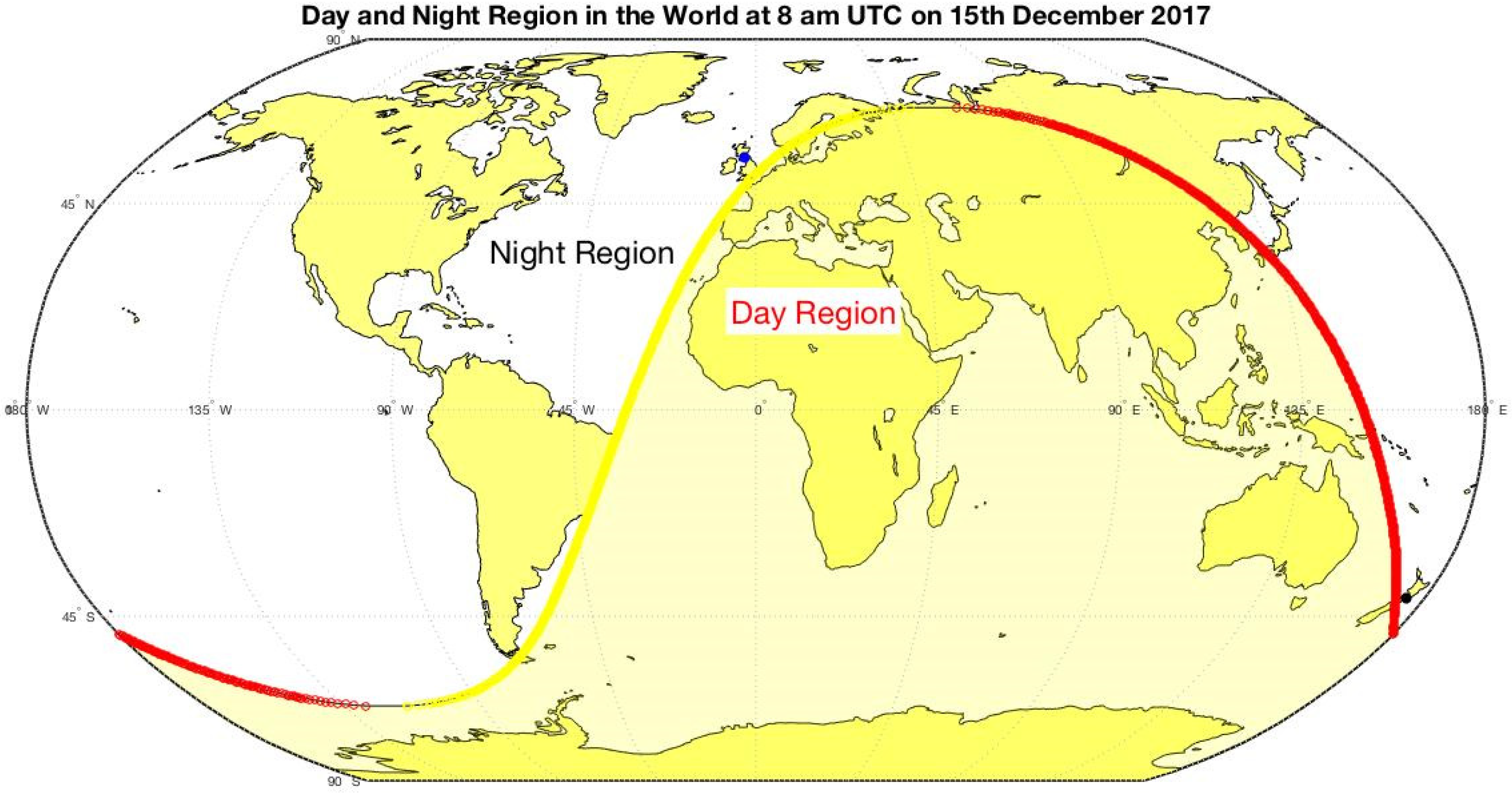
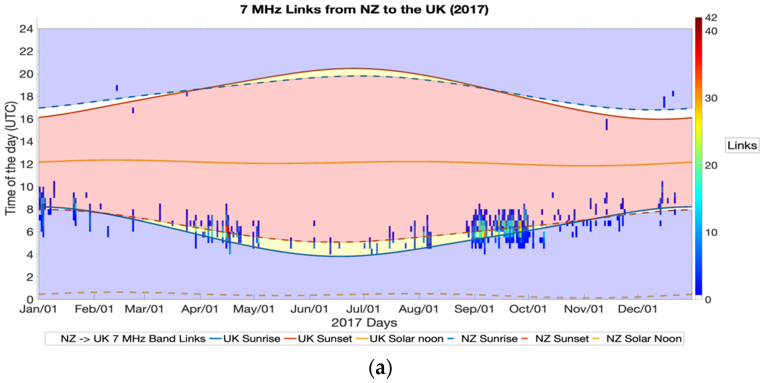
For very long-distance paths, such as between New Zealand and the United Kingdom, which are close to being antipodes, there are persistent reports that the radio wave propagation is significantly enhanced at dawn and dusk. This is known amongst the amateur radio community as “greyline propagation”—propagation of the radio signals along the terminator or simply entering the ionosphere and exiting the ionosphere at the terminator (sunrise/sunset) times (see Figure 1). An early reference from the Amateur Wireless magazine notes the propagation on wavelengths of 80 m and 95 m between the UK and New Zealand to be “best between 6.30 am and 7 am”, and they note that this is thought to be “because of the overlap of dawn and dusk” [2].

Interest in greyline propagation has lasted for over a century. It has been consistently reported by the amateur radio community (for example, [3,4,5]). A report from Callaway [6] shows radio communication links propagating between Florida and the Cocos Islands (near Sumatra) at a frequency within the 3.5 MHz band (80 m band). This communication link was interpreted to be greyline propagation because both locations were simultaneously located along the terminator [6]. Pontyatov et al. [7] presented research on super long-distance and round-the-world propagation in the HF bands communicating between various locations such as between Alice Springs (Australia) and Rostov-on-Don (Russia), and between Cyprus and Rostov-on-Don, using oblique ionospheric sounding. They indicated that the azimuthal angle of 10 to 25 degrees with the terminator is best for making a terminator propagation link.

These reports provide a motivation to conduct a more systematic long-term study. A new opportunity has arisen using the automated collection of radio amateur signals from the Weak Signal Propagation Reporter (WSPR) network [8]. The WSPR beacon network consists of thousands of beacon transmitters and observers, distributed over the globe with a prevalence in the northern hemisphere. The WSPR database is a very useful resource for radio science as it records the date and time of links made between two radio stations, as well as the callsigns and locations.

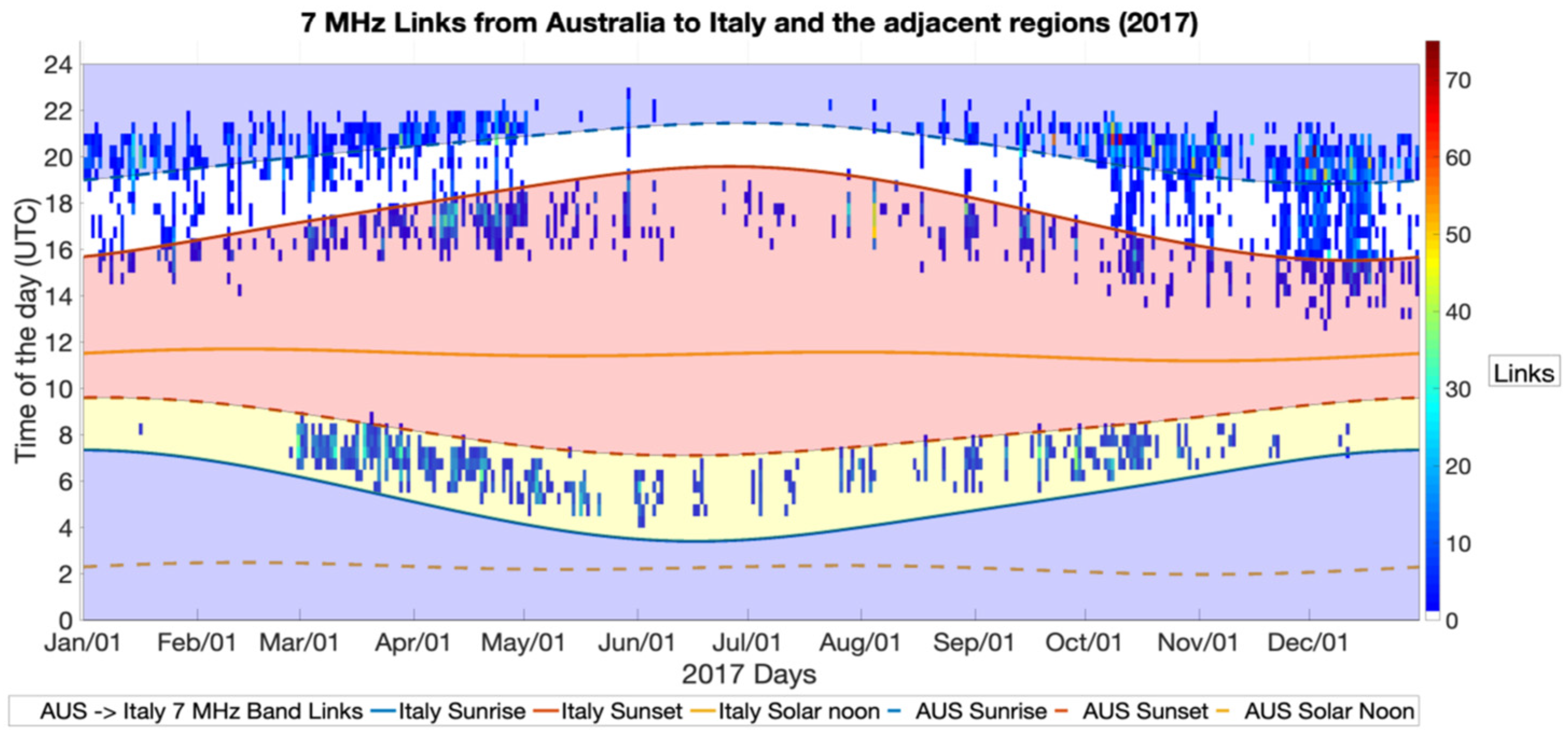
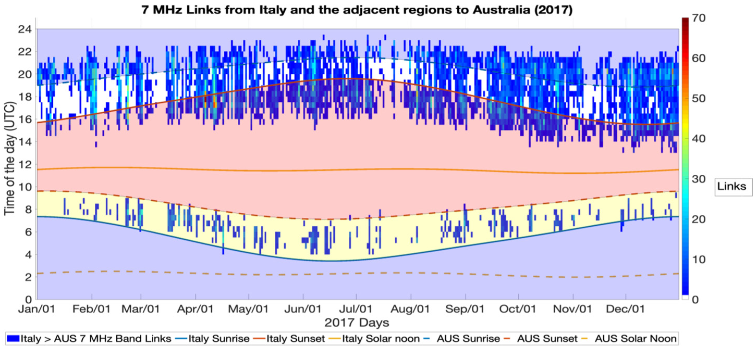
This paper aims to investigate the statistical pattern of long distance 7 MHz propagation between two countries that are coincident on the terminator line—the United Kingdom (UK) and New Zealand (Figure 1). Further observations between other locations such as Eastern Australia and Italy are included to augment these findings and to provide further insight.

It should be noted that due to the nature of amateur radio, much of the information available to scientists describing the amateur systems and data sets is not available in refereed scientific literature. Every effort has been made to reference technical reports as and where appropriate, but there is an inherent challenge in using amateur data for scientific studies. This aspect is discussed in the later sections of this paper.

2. The WSPR System and Data Set

The WSPR system consists of a large number of automated beacon transmitters and beacon receivers that are operated by radio amateurs around the world. Both the transmitters and receivers use the software-encoded WSPR radio protocol. Each transmitter sends out a coded message and each receiver reports the beacons it receives to a centralized database on the Internet, the WSPR database (wsprnet.org, accessed on 2 August 2022).

2.1. Beacon Transmission

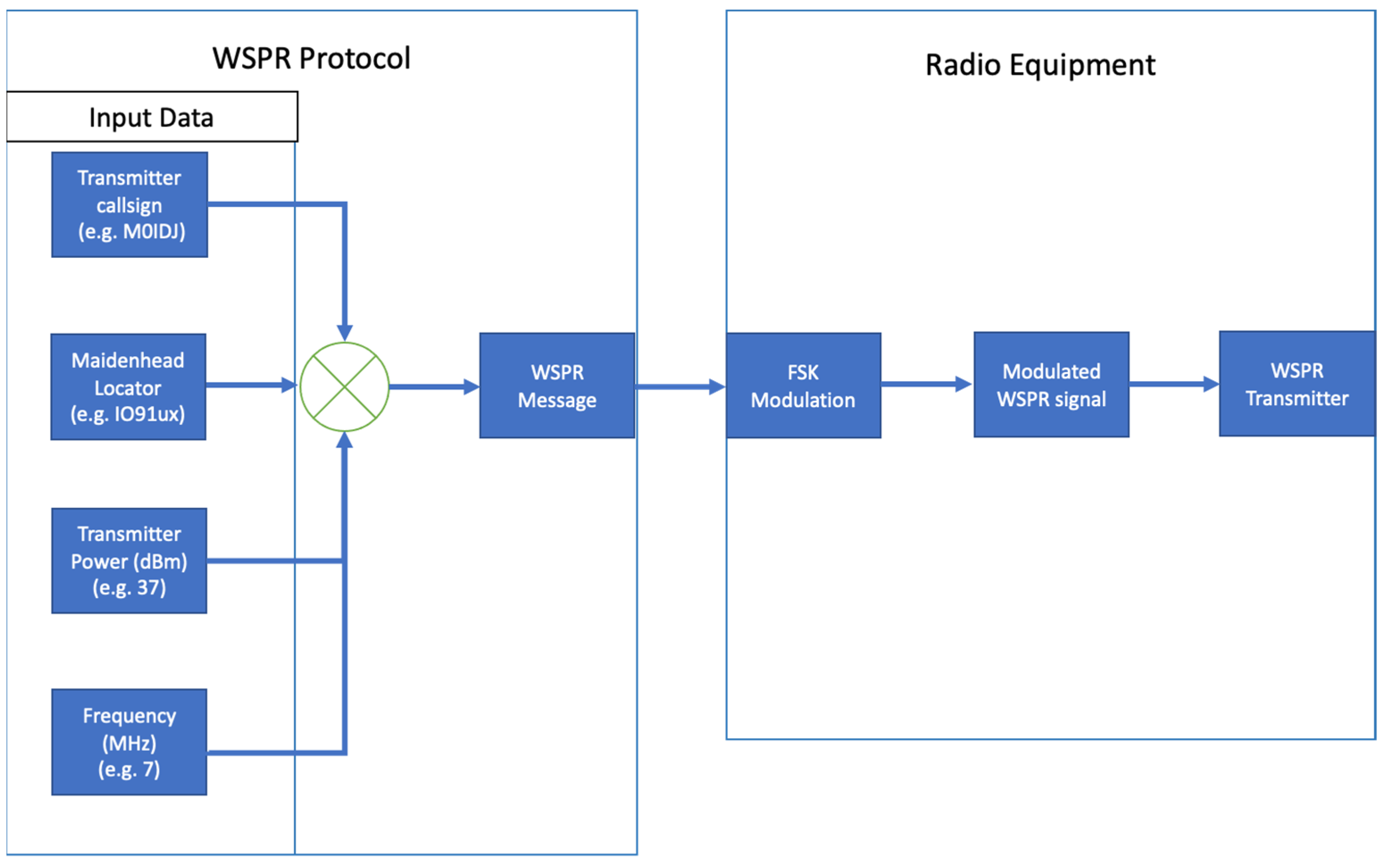
The WSPR signal comprises a message carrying the callsign, locator and transmitter power (input by the user within a total of 50 bits) which is encoded using Forward Error Correction (FEC) and interleaving [9]. The encoded message, which now has a total length of 162 bits, is then modulated onto the carrier signal using 4-Frequency Shift Keying (4-FSK) modulation at a rate of 1.4648 Baud. The total occupied bandwidth is approximately 6 Hz. It takes 110.6 s to complete a WSPR message, which is repeated every 2 min. The transmissions start 1 s after the even minutes of the hour, synchronized to an Internet time server via the Network Time Protocol (NTP). The beacon is silent during the remaining 9.4 s.

The beacon transmission is realized in software and can use the computer sound card to generate the modulated base-band signal (audio tones), which is transposed to the transmit frequency by means of an amateur radio single-sideband transmitter. The block diagram that describes the signal transmission is shown in Figure 2.

2.2. Frequency and Time Randomization

The WSPR protocol is used on specific frequencies in each of the amateur radio frequency bands (

Table 1. Frequency bands assigned to radio amateurs in the United Kingdom and the WSPR dial frequencies (not exhaustive).

Frequency Range	UK Amateur Radio Frequency Bands (MHz)	Frequency Band (MHz)	WSPR Dial Frequency (MHz)
LF	1.81–2.00	1.8	1.8366
HF	3.5–3.8	3.5	3.5926
	5.288–5.292	5	5.2872
	7.0–7.2	7	7.0386
	10.1–10.15	10	10.1387
	14.0–14.35	14	14.0956
	18.068–18.168	18	18.1046
	21.0–21.45	21	21.0946
	24.890–24.990	24	24.9246
	28.0–29.7	28	28.1246
VHF	50.0–52.0	50	50.2930
	144.0–146.0	144	144.4885

). The frequency band or set of frequency bands that an individual WSPR beacon uses depends on the capabilities of the individual amateur radio station. To help to mitigate against interference with each other, they can be assigned a frequency offset. A frequency segment of 200 Hz width is available for all WSPR beacons, which have a bandwidth of 6 Hz each. Additionally, the transmit time intervals are randomized, with each beacon transmitting in 25–50% of the available 2 min time slots.

2.3. Maidenhead Locator System

To share the latitude and longitude of the beacon in a compact form, the ‘Maidenhead locator’ is used. This method encodes coordinates of any location on the earth, expressed in the World Geodetic System 1984 (WGS-84), in a sequence of two letters, two figures and two letters. With these six digits, a location precision of 2.5 minutes of a degree latitude and 5 minutes of a degree longitude is realized, resulting in a position accuracy of approximately 3 km at mid-latitudes [10]. This system was proposed for amateur radio use by John Morris G4ANB and adopted by the IARU VHF Working Group in Maidenhead, England in 1980. The International Amateur Radio Union, Region 1, adopted it in 1982, and promoted worldwide use [11].

2.4. Beacon Reception

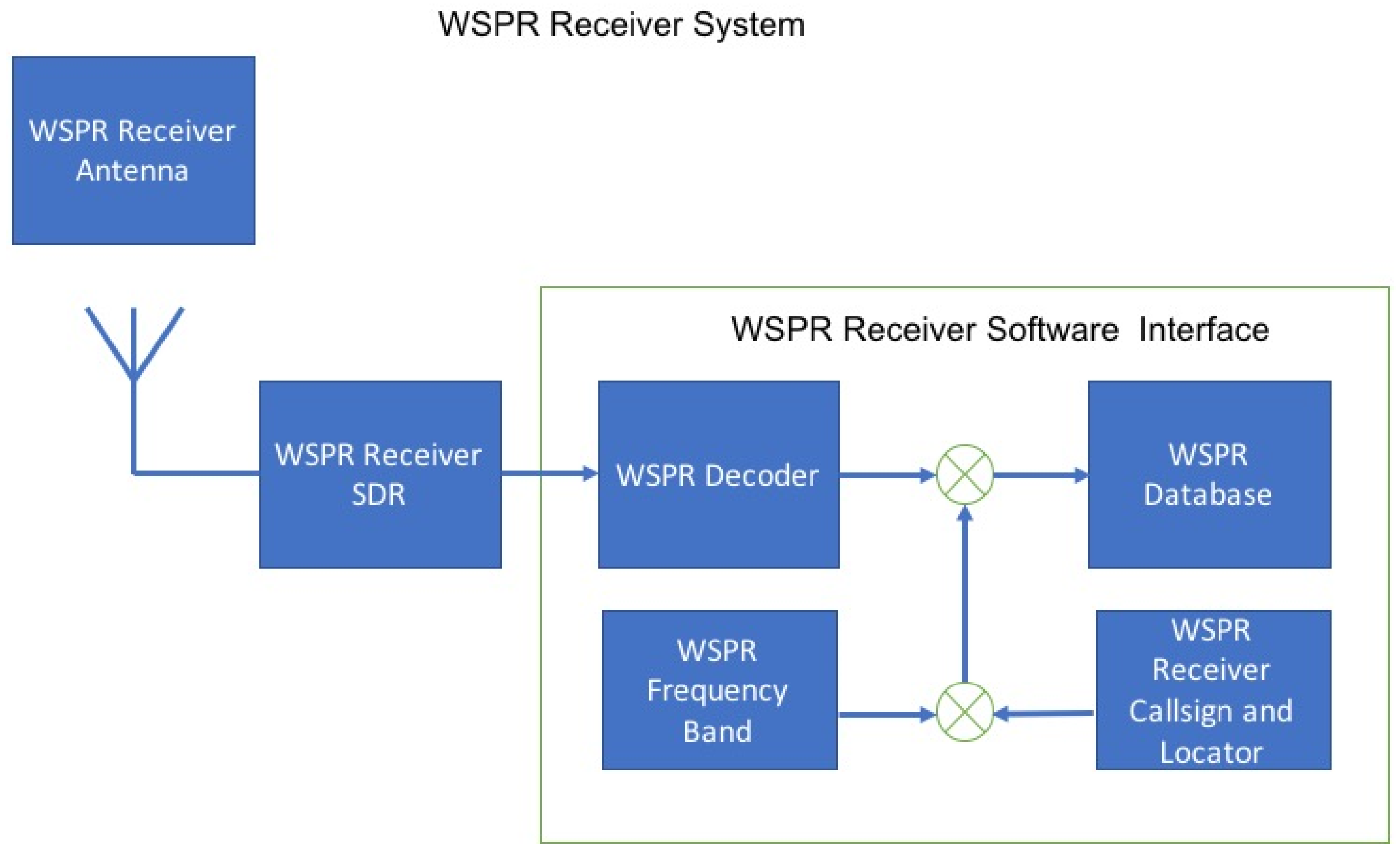
The WSPR receiver system consists of an antenna, a radio receiver, and the WSPR software in a computer, as shown in Figure 3. The WSPR system requires a timing synchronization to within +/−2 s of UTC at transmitters and receivers. This can be performed through the Internet but can also be set more accurately using GPS timing. It is crucial to ensure that the Internet connection is available, and the time synchronization in the computer is regularly updated for the successful operation of WSPR.

The receiver converts the WPSR signals to a baseband signal, after which the WSPR software (WSPR 2.0 or WSJT-X) analyses the 200 Hz frequency segments and decodes all WSPR beacon signals in it. Due to the narrow bandwidth of the signals and the FEC, signals can be decoded when their SNR is greater than −34 dB, referenced to a 2500 Hz receiver bandwidth, with a 50% probability of decoding at −31 dB if the Doppler spread is below 0.01 Hz. The WSJT-X software also performs a second pass, after coherent subtraction of the signals decoded during the first pass. This increases the likelihood of decoding overlapping transmissions.

The callsign, power, and Maidenhead locator of each beacon is recovered from the received WSPR messages. An SNR value derived from the error correction algorithm is recorded. The relative frequency drift between transmitter and receiver is also established in the software. The Maidenhead locator and receiver callsign, which are pre-set by the owner of the receiver, are also added to the record. Finally, using the location of the transmitter and the receiver, the short-path great-circle distance and azimuth are calculated by the WSPR software and stored in the same record. This is performed for each received beacon signal. The records are then uploaded to the WSPRnet website via an Internet connection. If the computer on which the WSPR software runs is offline, the receiver will not be able to report the signal into the WSPR database even if the receiver is active.

The WSPR data recorded into the WSPR database is saved as a CSV file on a monthly basis. The CSV file records the WSPR data in 15 columns, and each column represents the data that the WSPR protocol has decoded, as listed in

Table 2. WSPR data columns and the type of the recorded data.

Column Number	Type of Recorded Data	Example	Source
1	SpotID	736696460	Receiver
2	Timestamp	1488778440	Receiver
3	Receiver’s Callsign (Reporter)	G3ZIL	Receiver
4	Receiver Location (Reporter Grid)	IO90hw	Receiver
5	SNR (dB) from the receiver	−25	Receiver
6	Frequency (MHz)	7.040102	Receiver
7	Transmitter Callsign (Call)	ZL3PX	Transmitter
8	Transmitter Location (Transmitter Grid)	RE66hm	Transmitter
9	Power (dBm)	47	Transmitter
10	Drift (Hz)	−1	Receiver
11	Distance (km)	19071	Receiver
12	Azimuth (degrees)	334	Receiver
13	Band (MHz)	7	Receiver
14	Version	1.7.0-rc1	Receiver
15	Code	0	Receiver

.

3. Method

3.1. Data Selection from the WSPR Database

Observations stored in the WSPR database for the year 2017 are used in this study. A full year is selected to investigate seasonal variations. It was decided not to use multiple years, to avoid the influence of the solar sunspot cycle. The selected year is in the descending half of the sunspot cycle 24.

Only observations on 7 MHz are used, as the largest number of observations was available on this frequency band. Greyline propagation enhancements are reported on frequencies between 1.8 and 10 MHz, but only a limited number of radio amateurs have the necessary antennas for long-distance propagation on frequencies below 4 MHz.

The WSPR data used in this project were analyzed to select radio links between locations of interest. This was performed by first filtering the WSPR records by transmitter and receiver call signs, which identify their countries. Then, the resulting data were further filtered using the two-letter prefix of the Maidenhead locator. For example, the starting prefixes for the UK locations are ‘IO’ and ‘JO’, as shown in

Table 3. Maidenhead locators starting prefixes of the locations.

Locations	Maidenhead Locator Prefixes
United Kingdom	IO, JO
New Zealand	RE, RF
Europe	IN, JN, KN, IM, JM, KM, IO, JO, KO, IP, JP, KP
Eastern Australia	QH, QG, QF QE

.

3.2. Statistical Analysis and Graphical Representation

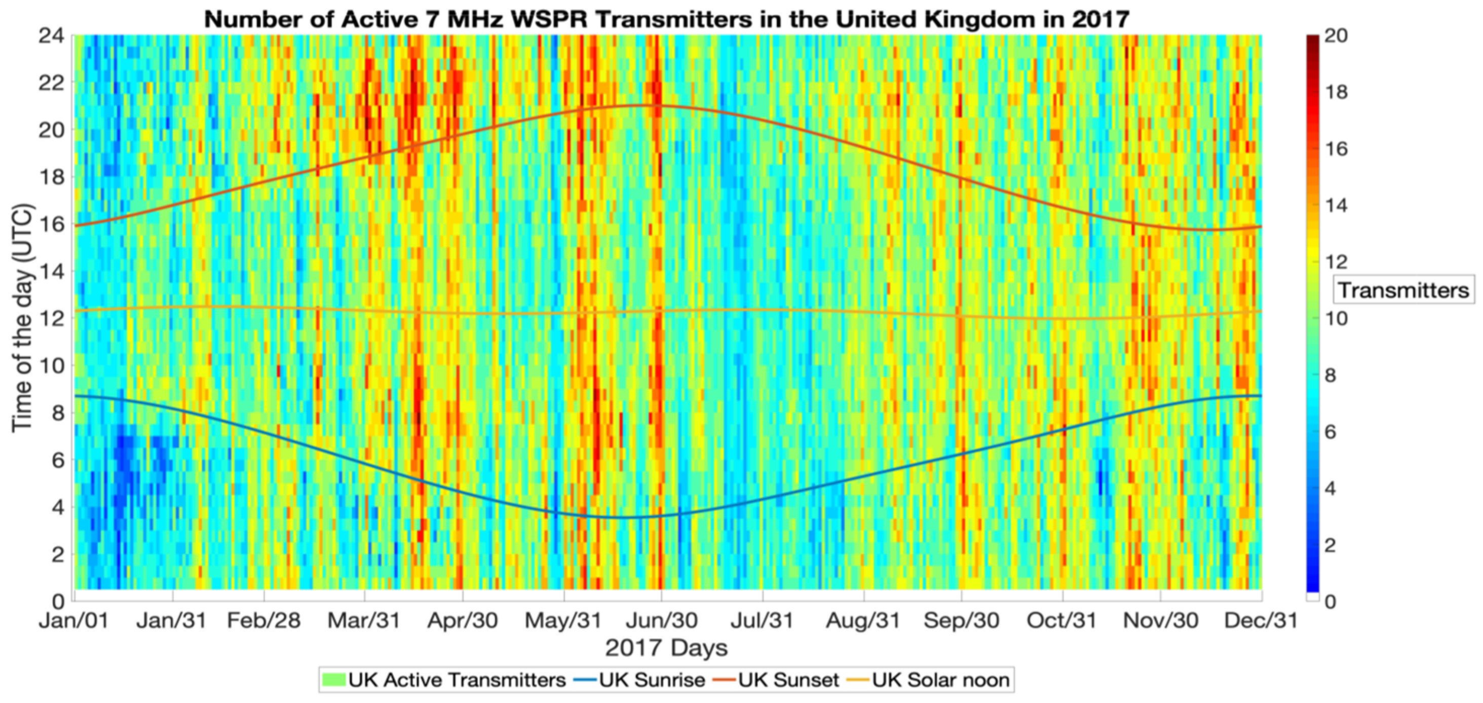
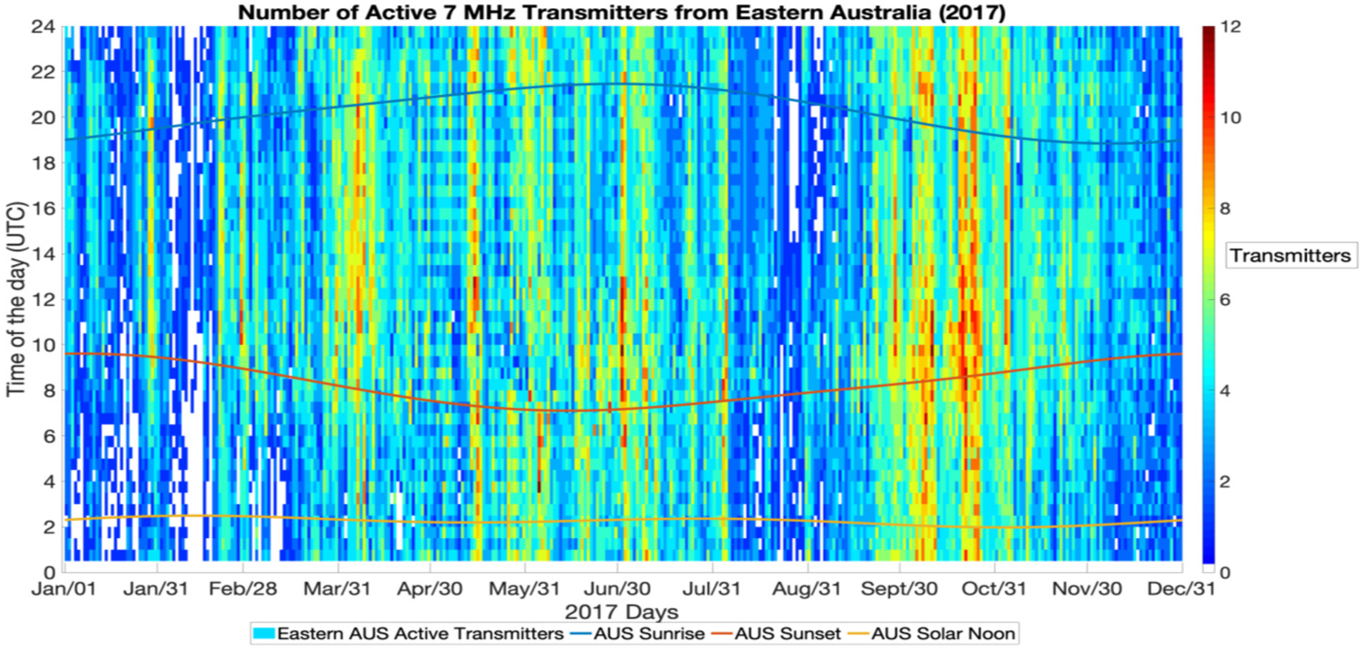
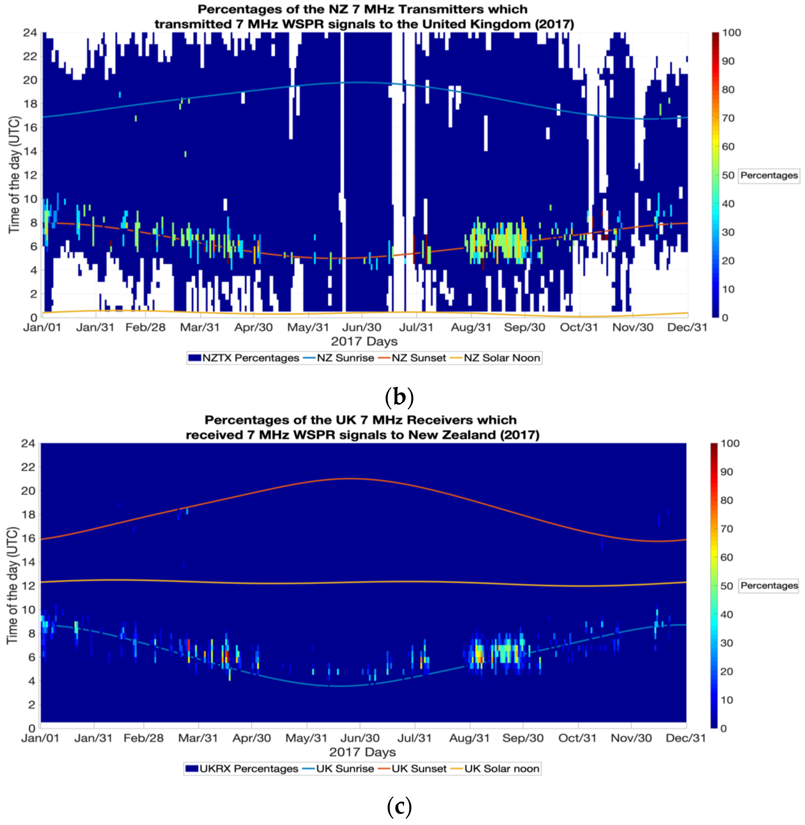
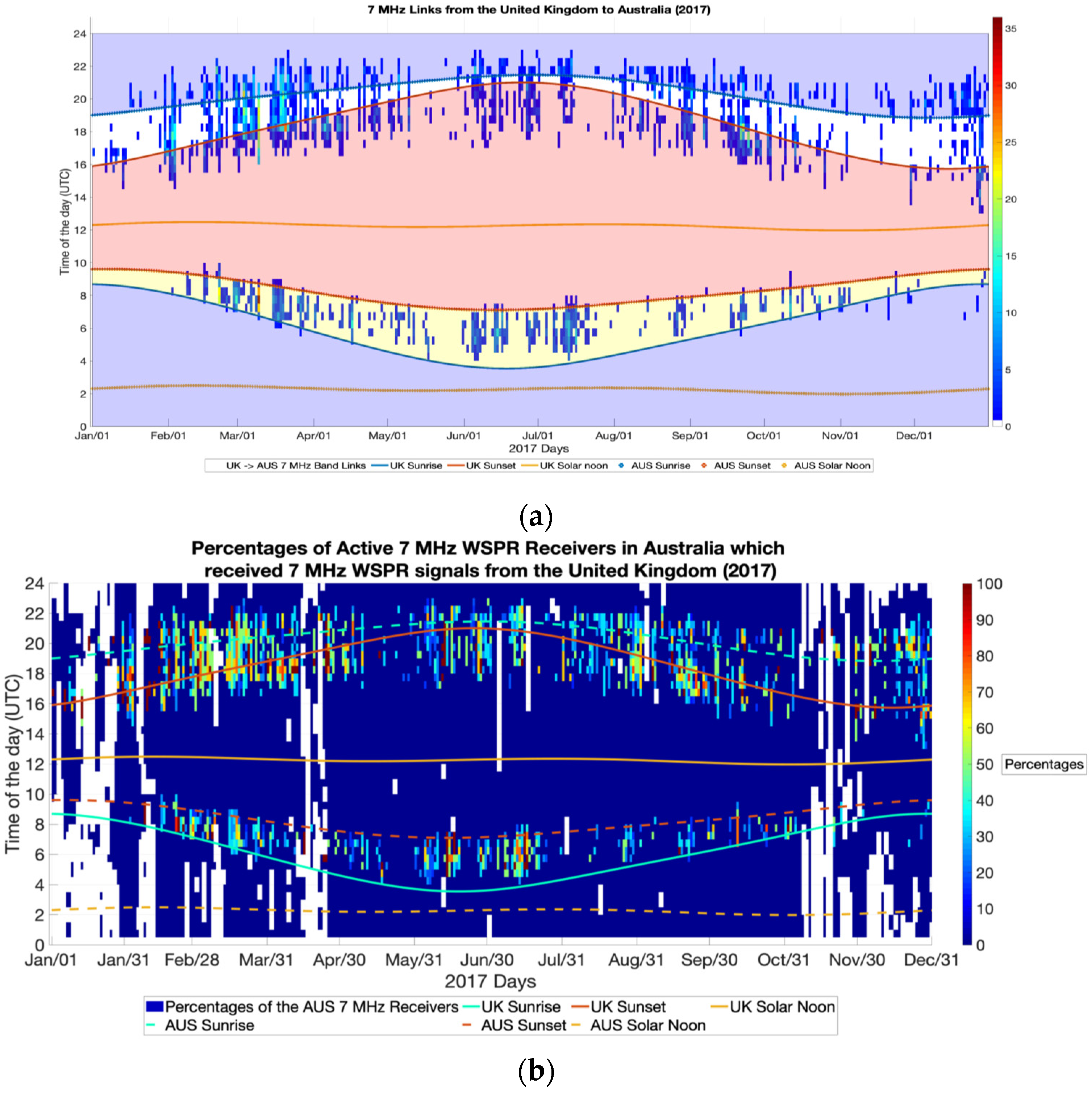
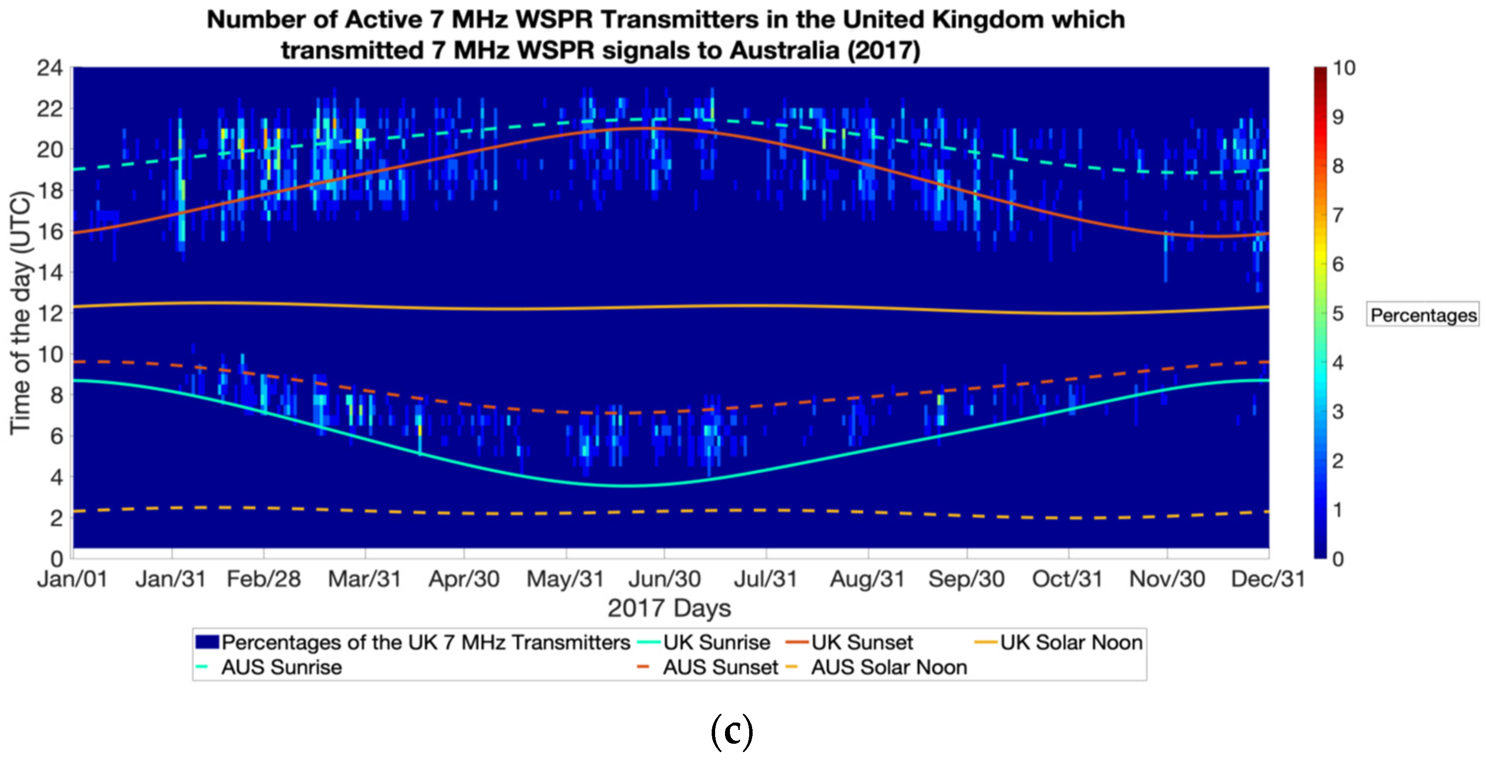
After this selection by year, frequency and geographical location, the number of observed radio links from beacons in one geographical area to receivers in the other geographical area is counted for each half hour of each day. This is performed twice, e.g., once for transmissions from the United Kingdom to New Zealand and once from New Zealand to the United Kingdom, to investigate any asymmetry. These accumulated results are then plotted in a Cartesian diagram where the horizontal axis represents the day of the year and the vertical axis the UT hour of the day. The number of links in each half hour is represented using a color scale. The same representation can also be used to present the hours in which a beacon transmitter or receiver was active. This is important as the WSPR beacons may be switched on and off at will by the amateur radio operator. The number of observations relative to the number of beacons and receivers that are active is an indication of suitable radio wave propagation.

3.3. Challenges of Using the WSPR Data Set

Using the WSPR data set poses several challenges. For each studied case, it is important to determine if sufficient beacons and receivers are operating, so that the patterns in observed radio links can be attributed to propagation conditions or potentially to other causes.

WSPR provides a centralized database for the radio amateur community to upload their records. The records rely on the transmitter and receiver locations being correctly input into the software. It is noted that the WSPR information could be inconsistent due to human error in the recording. When using this data for science, it is important to use multiple sites (hence, checks can be made for consistent results between similarly located beacons or receivers) and to check consistency between call sign and recorded locations of transmission and reception. The https://www.qrz.com (accessed on 2 August 2022) website may be used to verify station locations, but information on this website is voluntary, not centrally orchestrated and is updated only from time to time by the individual amateur radio operator. Reliable up-to-date equipment information cannot necessarily be found on this website.

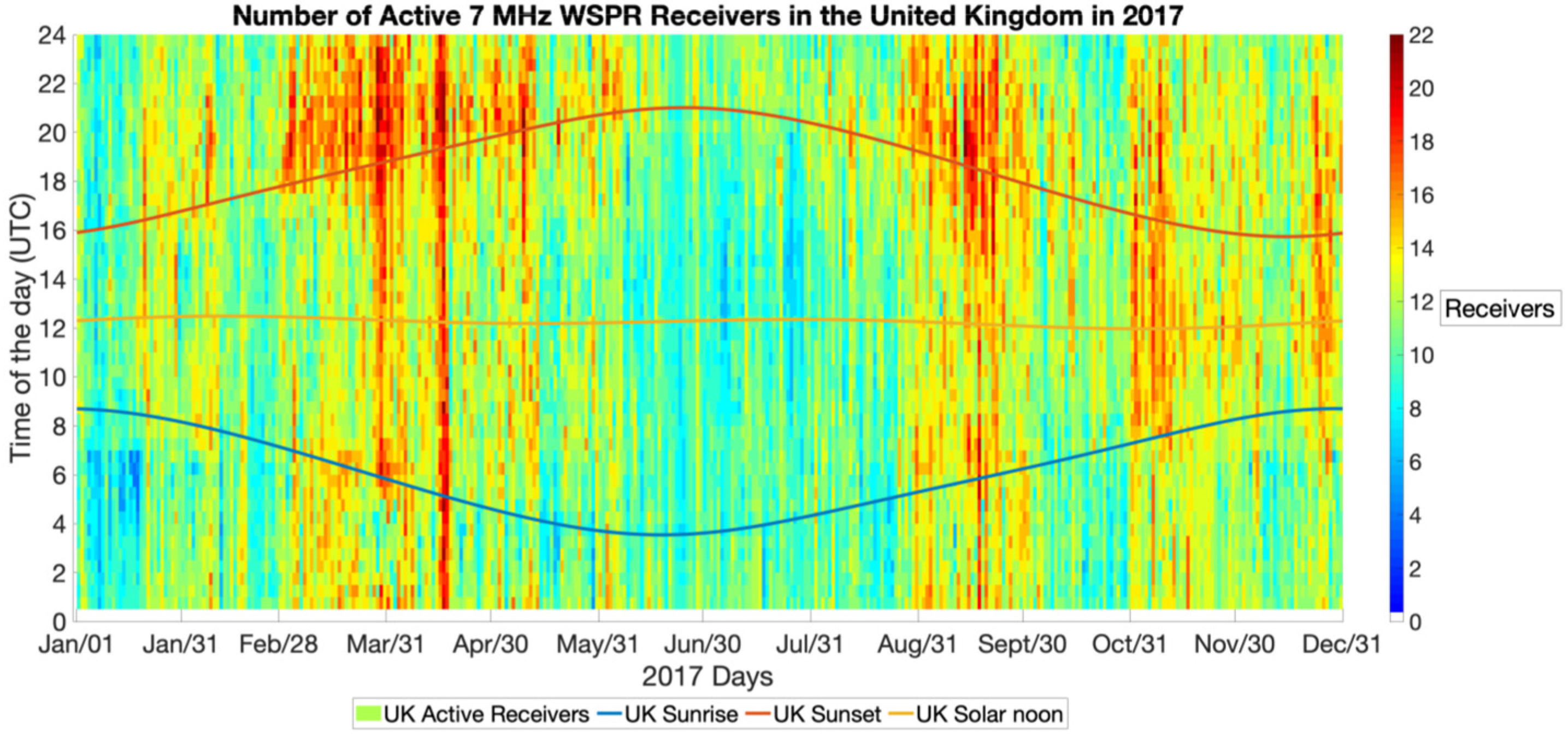
There is no official recording of the operating schedules for WSPR equipment (beacons and receivers), so there may be times when equipment is not operating. Care is needed to ensure that the operation schedule of equipment is not mis-interpreted as a pattern in the propagation conditions. However, a check can be made to verify times when a particular transmitter is active by checking if it was recorded at a receiver anywhere, or to verify times when a particular receiver is recording signals from anywhere. This can then serve to inform the analysis and to build confidence in the availability of operating equipment. As an example, the activity from the radio transmitter with callsign ZL3TKI is presented in Figure 4 and Figure 5.

It is also possible that a communication link cannot be made due to signal reception at the receiver being below the SNR threshold for WSPR, which is around –34 dB. The weakest signal that can be decoded by an individual receiver depends on the effectiveness of its antenna, the antenna location and the local noise level.

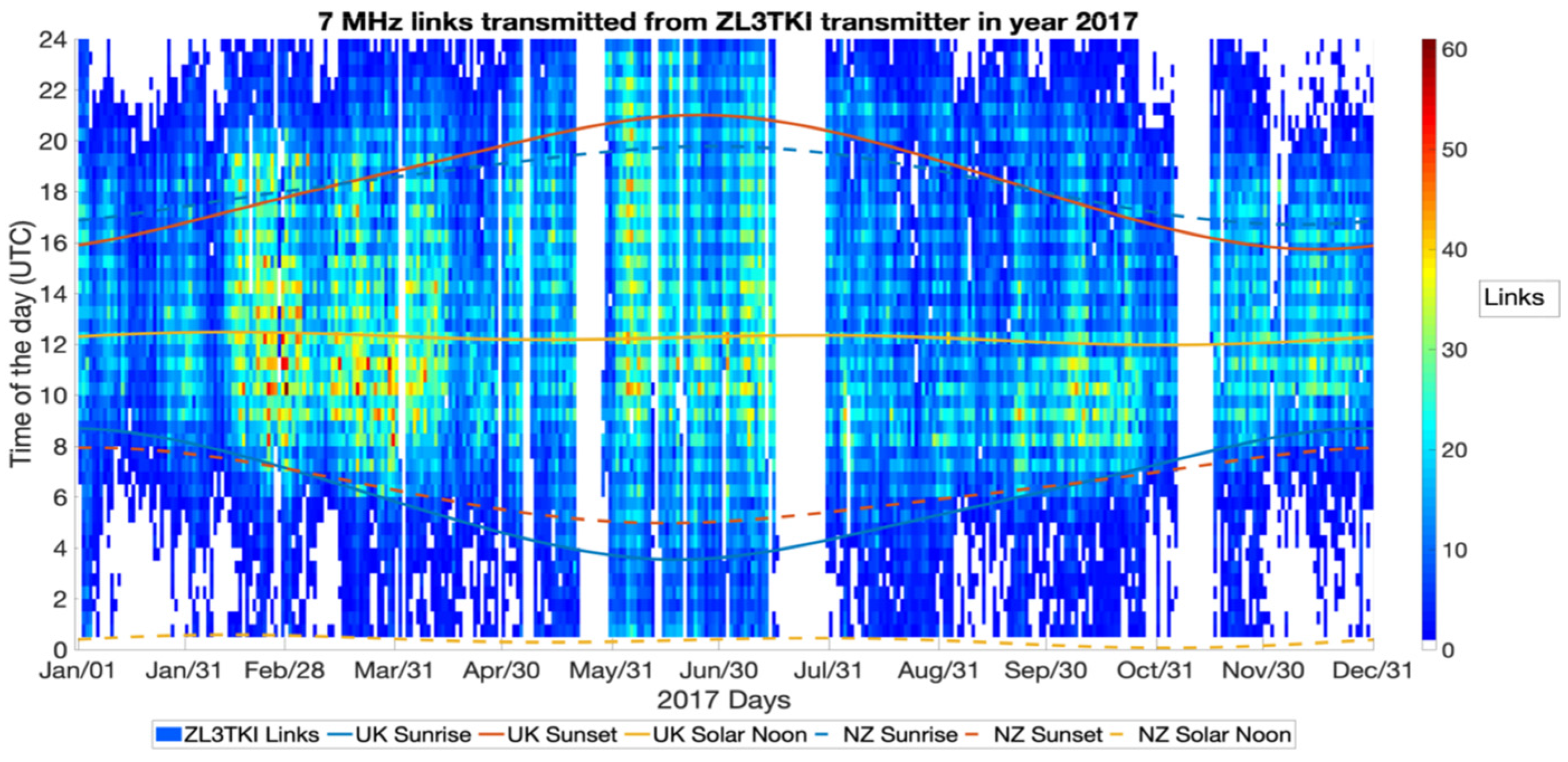
Figure 4 shows the reception of links transmitted from the radio station ZL3TKI. The x-axis represents the day of the year (2017) and the y-axis represents the time of the day in UTC hours. The solid lines are the UK’s sunrise (blue), sunset (red) and solar noon (yellow) hours. The dashed lines are the New Zealand’s sunrise (blue), sunset (red) and solar noon (yellow) hours. These are defined by the locations on the ground for a particular receiver location defined from the median of the actual receiver location. The colors are total numbers of links received.

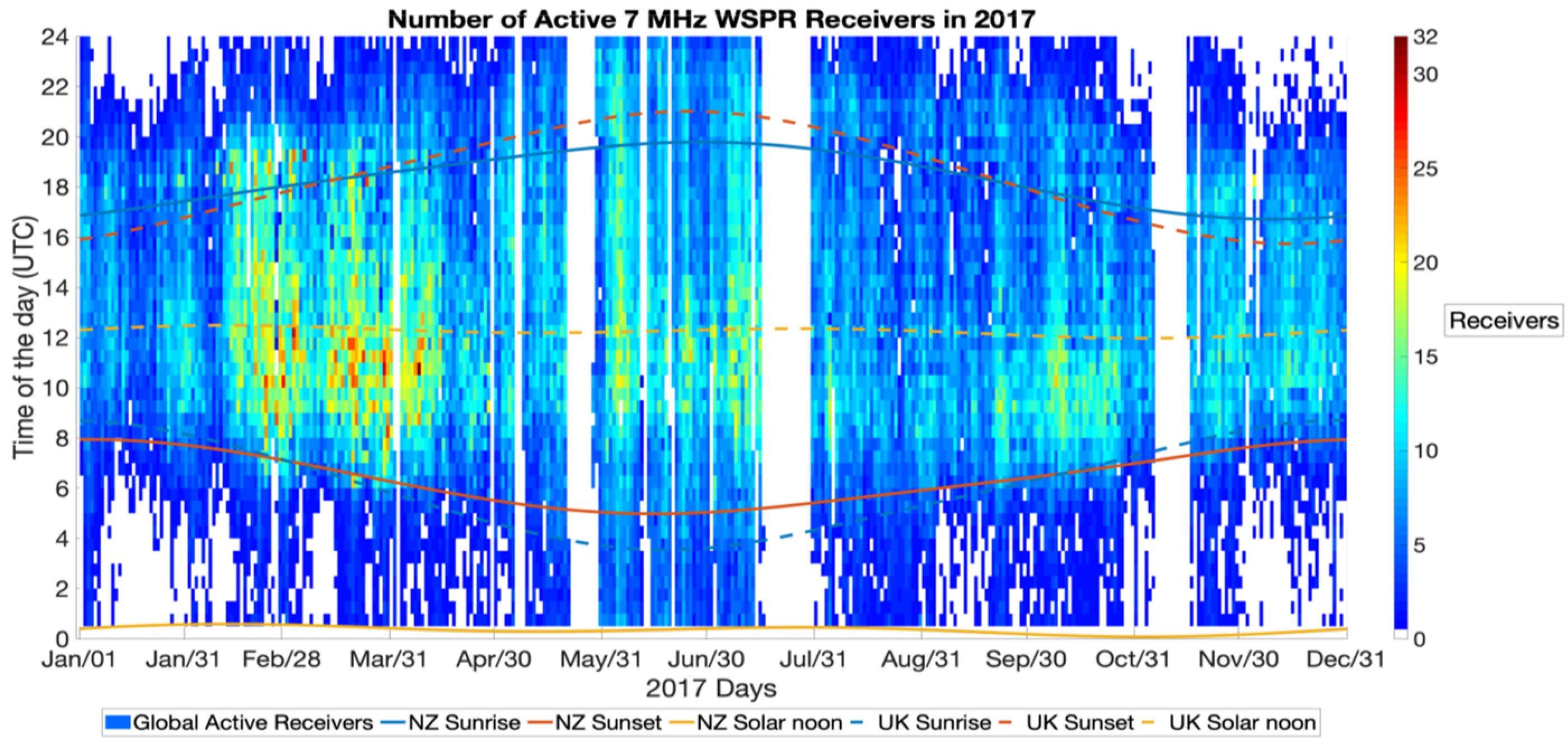
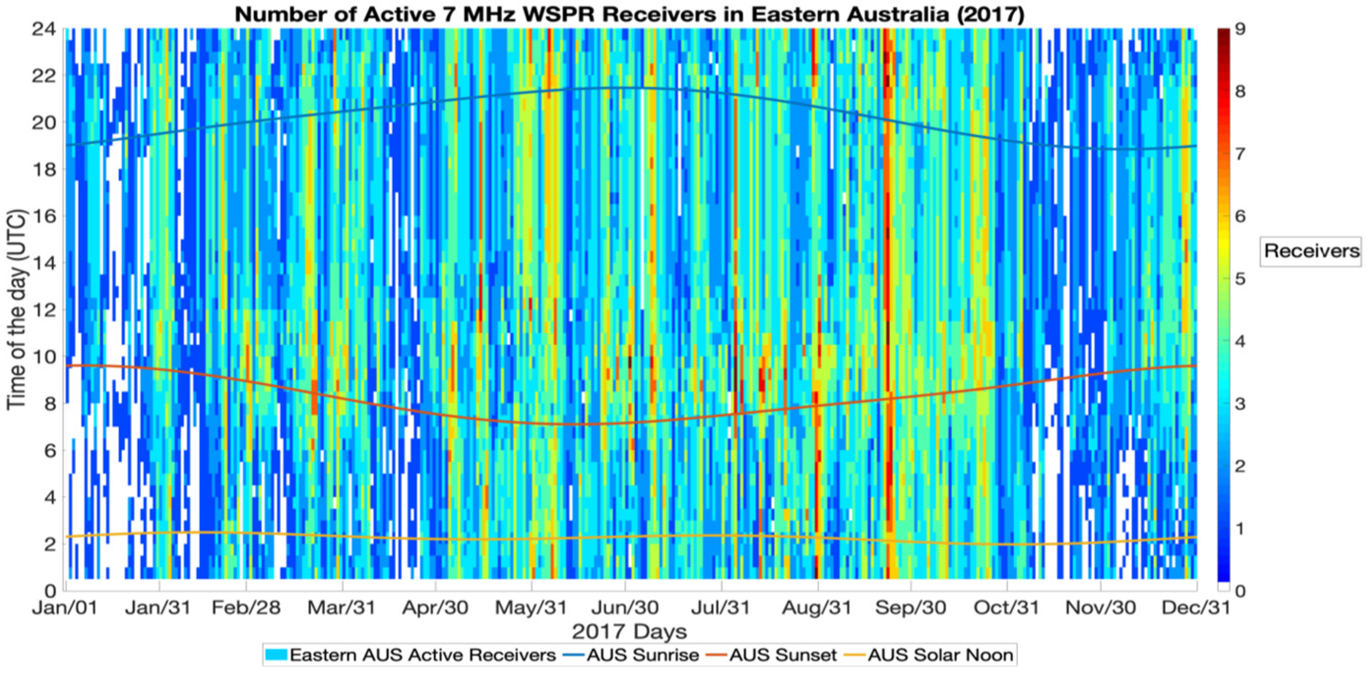
Figure 5 shows the number of active receivers globally that (had at any time) made a link with ZL3TKI. The solid lines are the New Zealand’s sunrise (blue), sunset (red) and solar noon (yellow) hours. The dashed lines are the UK’s sunrise (blue), sunset (red) and solar noon (yellow) hours.

From Figure 4, we can conclude that the beacon transmitter ZL3TKI was transmitting for most of the entire year and 24 h per day. Figure 5 shows the receiver availability. Note that transmissions are not made in every possible 2 min window, but multiple transmissions can be made within a half-hour window.

Despite the noted challenges with the use of WSPR for scientific study, the data can be used for radio propagation analysis, since they are from a global radio station network, and the large number of stations can be used together to infer statistical information.

4. Results

4.1. Availabilty Statistics

It is important to analyze the number of active stations throughout the year that will be used to gather the statistical information about the radio links.

Table 4. Number of radio stations which have established links between the UK and New Zealand, and between the UK and Eastern Australia in the WSPR database in 2017. Eastern Australia was added in to achieve similar numbers of transmitters and receivers.

Countries	Number of Recorded Call Signs
UK	91 transmitters 121 receivers
New Zealand	21 transmitters 26 receivers
Eastern Australia	68 transmitters 76 receivers

notes the number of different callsigns noted throughout the year on 7 MHz. Figure 6 shows the number of active UK transmitters in each half hour. These are found by searching the WSPR database for records of transmitters in the UK, considering all geographical regions for reception. Figure 7 is the corresponding record for active UK receivers (again, regardless of where signals were received from). Figure 8 and Figure 9 show the corresponding pair of figures for New Zealand, and Figure 10 and Figure 11 for Eastern Australia. Taken together, these figures show the availability of operational equipment throughout the year.

4.2. Successful Communication Statistics

We have shown in Section 4.1 that when both New Zealand and Eastern Australia are considered together, there are sufficient active transmitters and receivers throughout the year to investigate the statistical occurrences of links being made.

Figure 12 shows the radio links made between New Zealand transmitters and UK receivers. The x-axis represents the day of the year (2017), and the y-axis represents the time of the day in UTC hours. The red shaded area represents the UK daytime hours, and the blue shaded area is the New Zealand daytime hours. The yellow shaded area shows the common daytime hours, and the white shaded area shows the common night hours. The solid lines are the UK’s sunrise (blue), sunset (red) and solar noon (yellow) hours. The dashed lines are the New Zealand’s sunrise (blue), sunset (red) and solar noon (yellow) hours. These are defined on the ground (not at ionosphere height) and the geographical coordinates used are the median values of the actual receiver locations. From Figure 12a, it is evident that most of the links are made at times close to the UK sunrise. Figure 12b shows the percentage of active transmitters in New Zealand that made links to the UK. The times when there are no active transmitters are depicted as no color (white). Figure 12c shows the percentage of active UK receivers receiving a signal from New Zealand.

Taken together and comparing back to the earlier figures referred to in Section 4.1 showing the availability, it can be seen that there is a preference for signals to be received around sunrise in the UK. Comparing Figure 12a back to Figure 7, the availability of UK receivers is not clustered around sunrise but is distributed throughout the day. Comparing back to Figure 8, the availability of New Zealand transmitters is not clustered around (UK) sunrise but is distributed throughout the day. Therefore, the result is not an artefact of equipment availability. Moving to Figure 12b, this provides further indication that there is a preference for New Zealand transmitters to link through to the UK around sunrise. Figure 12c shows that the highest percentages of UK receivers that received from New Zealand were around the UK sunrise.

To supplement and strengthen the findings from the New Zealand results, Figure 13 shows the links made between Eastern Australia transmitters and UK receivers. From Figure 13a, it is evident that almost all of the links are made at times close to the UK sunrise, but particularly at times of common daylight. In the (UK) evening, there are links close to the terminator time but less during the time of common darkness and less during (UK) summer. Figure 13b shows the percentage of active transmitters in Eastern Australia that made links to the UK.

Figure 13c shows the percentage of active UK receivers receiving a signal from Eastern Australia. Taken together and comparing back to the figures referred to in Section 4.1 (Figure 7 and Figure 10) showing the availability, it can be seen that there is a strong indication for a preference for signals received around the terminator times, but not during the common night-time. To put this another way, it seems that in addition to a terminator preference, most successful links have started and/or ended in the daytime.

Figure 14 shows the links made between UK transmitters and New Zealand receivers. From Figure 14a, it is evident that almost all of the links are made at times close to the sunrise or sunset. Figure 14b shows the percentage of active transmitters in the UK that made links to New Zealand. Figure 14c shows the percentage of active New Zealand receivers receiving a signal from the UK. Taken together and comparing back to the earlier figures referred to in Section 3.1 (Figure 6 and Figure 9) showing the availability, it can be seen that there is a strong indication for a preference for signals received both around sunrise and sunset.

Figure 15 shows the links made between UK transmitters and Eastern Australia receivers. From Figure 15a, it is evident that almost all of the links are made at times close to the sunrise or sunset. Figure 15b shows the percentage of active transmitters in the UK that made links to Eastern Australia. Figure 15c shows the percentage of active Eastern Australia receivers receiving a signal from the UK. Taken together and comparing back to the Section 3.1 figures showing the availability, it can be seen that there is a preference for signals to be received around sunrise and sunset. It is interesting to note that the UK morning time links are confined to the common daytime hours, whereas the UK evening links are spread across the common night and also into the times, where there is one end of the link in the daytime and the other end in the night. Comparing back to the link in the other direction (Figure 13) there seem to be more common night-time links in Figure 15.

The results from UK to New Zealand showed links in both the sunrise and sunset, whereas the New Zealand to UK direction showed a preference for sunrise. This finding is supported by the Eastern Australia to UK result, but only during the UK summer sunset period.

Figure 16 shows the Eastern Australia to Italy direction and Figure 17 the Italy to Eastern Australia. Going from Australia to Italy, we see a sparsity of received signals in the European summer evening and also in the winter morning. In the opposite direction, we see a more even spread throughout the year. There is some evidence from Figure 10 that there are fewer transmitters in Eastern Australia in the (Europe) wintertime, but there are transmitters available in the (Europe) summer evening. The receiver availability (Figure 11) is largely spread evenly throughout the year.

4.3. Local Noise

The results in Section 4.2 initially seemed to suggest an asymmetry in the propagation mechanism. While this may be possible, it would be an unexpected finding because, for a given link at a given time, ionospheric conditions that support propagation in one direction should also support it in the other direction. An alternative explanation could that there are different local noise levels at either end of the links. A possible hypothesis is therefore that the ambient electromagnetic noise in the European/UK region is elevated during the sunset hours of the summer, and this is inhibiting the reception of the radio signals during this particular time period.

The WSPR measurements provided SNR measurements at the reception, but they do not directly measure the local noise. Nevertheless, recent measurements of HF radio noise have started to be taken through the projects run by radio amateurs, such as the radio noise measurements measured by a radio amateur with the callsign OE9GHV from Rankweil, Austria, from October 2020 to May 2021, as shown in Figure 18. These measurements were made in a remote location near the border of Switzerland and Austria. We can use this to examine the general trends throughout the day and year.

Figure 18 indicates that the noise in the evening is at the maximum during spring, and shows that there is an asymmetry between the noise measurement between the morning and the evening hours. This provides some support for the hypothesis that elevated noise might be inhibiting the summer sunset reception of WSPR signals in Europe. It is important to note that as these noise measurements are taken in a remote rural location, this is electromagnetic noise generated by far-away thunderstorms and man-made noise from distant cities, received via ionospheric propagation [13]. In urban areas, noise generated by electrical and electronic appliances will be dominant. However, most man-made noise in cities is also generated in the evenings, when a larger number of appliances are in use.

5. Discussion and Conclusions

This paper has demonstrated the use of WSPR citizen science data for the scientific study of HF radio propagation. The challenges of using WSPR were explained, and the availability of observations allowed us to provide context to interpret the results. This paper demonstrates a new measurement technique that has revealed, for the first time, a temporal and seasonal pattern to the long-distance radio propagation at 7 MHz. The patterns show systematic preference for propagation around the terminator times, with seasonal variations and asymmetry in the sunrise/sunset results. While the greyline propagation phenomenon is a topic of active discussion in the amateur radio community, scientific research into this domain has been minimal due to a lack of systematic observations and records. This paper fills that gap and represents a new statistical finding in the scientific literature.

The terminator region of the ionosphere (sunrise/sunset) is shown to support 7 MHz radio propagation preferentially over other times of day. The sunrise/sunset ionosphere is known to have very strong horizontal gradients in electron density and rapid temporal changes in the vertical profile structure in the transition from day to night, or night to day. However, the sunrise/sunset ionosphere is currently not well characterised in ionospheric models, and it is difficult to take measurements on a global scale. Verhulst [14] highlights that at sunrise/sunset, not all ionospheric altitudes are exposed to the first/last sunlight of the day at the same time and that this complicates the modelling process. Their study focusses on a local region (Dourbres, Belgium) where ionosonde observations are readily available to constrain and assist in advancing their model. Our study reveals a global perspective on the sunrise/sunset region of the ionosphere because the sunrise/sunset regions are supporting refraction of the HF signals in a way that is amenable to long-distance propagation. These new global-scale results are important because they provide an insight into the seasonal variation of ionospheric gradients at sunrise/sunset that could be used to constrain and improve future ionospheric models.

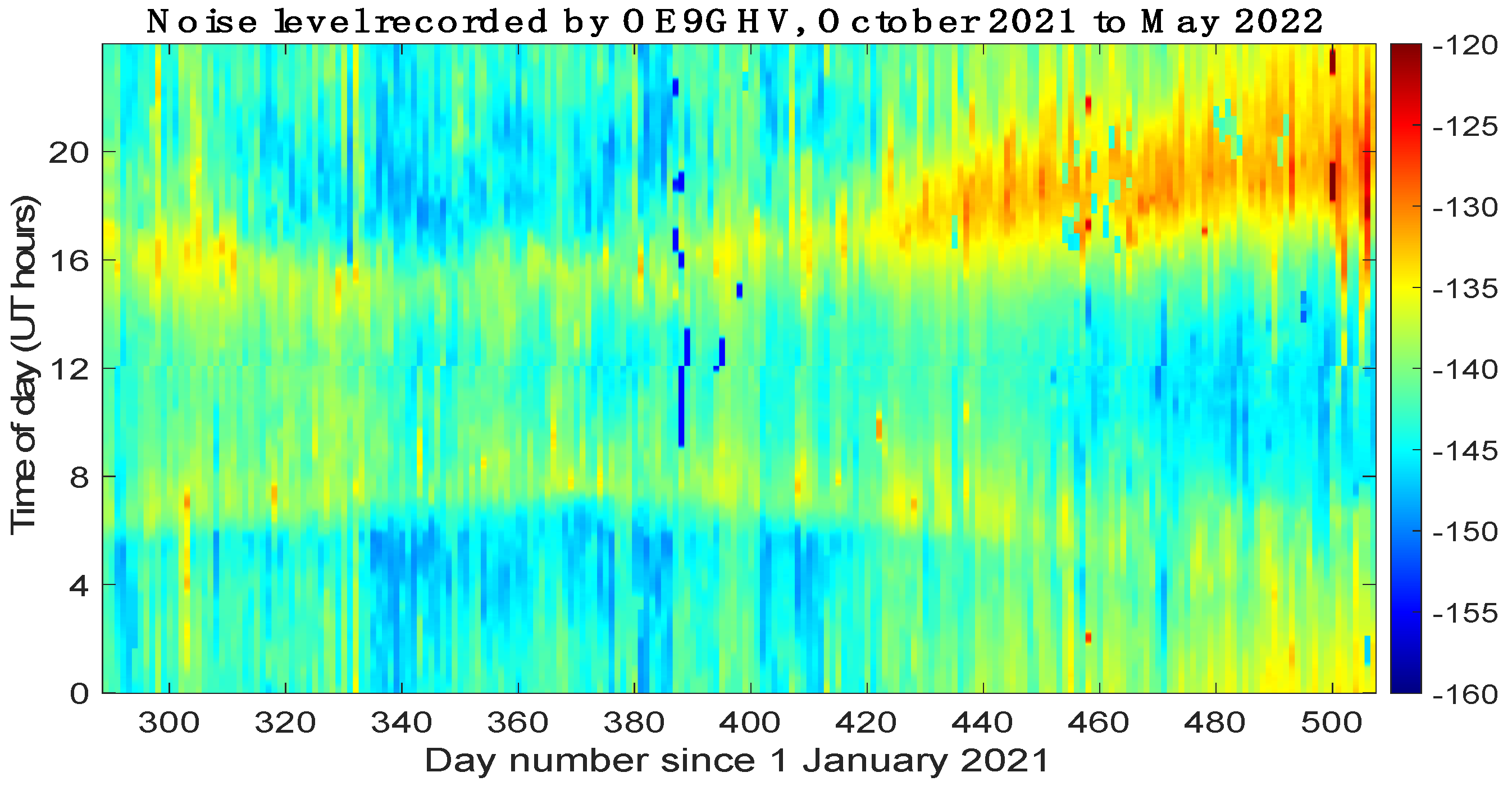
Some interesting asymmetries were evident in the propagation results. In particular, the New Zealand-to-UK links were almost only found around UK sunrise, whereas the UK-to-New Zealand links were found around UK sunrise and UK sunset times. This finding was supported by additional investigations between Australasia and Europe. A possible explanation for the lack of signal reception in the European/UK summer sunset may be related to the elevated HF noise levels. There is some evidence to support a hypothesis that the seasonal/temporal variation of noise in Europe may elevate the noise levels at times that tie in with the lack of WSPR reception around sunset. The correct characterisation of the noise is important if HF ionospheric observations are to be used to infer information about the ionosphere itself.

One very interesting aspect that might have a significant effect on the WSPR statistics is the Doppler spreading of the signal. Transmissions could reach the receiver of interest, but they may still not be decoded if they have encountered ionospheric conditions that have caused a Doppler spread that is a significant fraction of the signal bandwidth. This particular effect would not manifest in a way to show the directional asymmetry as reported in this paper, so it is not of concern in the interpretation of our results. Nevertheless, it would be an important consideration in other future statistical investigations using the WSPR database.

This paper has demonstrated clear evidence for greyline propagation and while that is a significant milestone, in many ways it opens up further questions. These questions relate to how the propagation patterns will look across other HF radio frequencies, for other paired locations and for other years throughout a full solar cycle remain open and can soon be addressed with the WSPR and other similar amateur radio data sets. The methodology developed here could support a much more comprehensive study multi-year and multi-frequency on long-distance HF propagation on a global scale that has never before been possible.

It is recognised that while amateur radio observations are not using scientific instrumentation and are not designed for rigorous investigations, in some way, this is offset by their availability, distribution and ease of access. Provided that care is taken to design a study that is robust to individual equipment operation outage, interesting and useful insights into ionospheric propagation can indeed by achieved with amateur radio equipment. There have been other papers demonstrating the wider utility of amateur radio signals for ionospheric study and they are starting to yield scientific results. Notably, in the innovative use of WSPR, Frissell et al. [15] examine the properties of large-scale ionospheric waves and show that amateur radio signals offer a tracer of the waves through their modulation of the communication distance.

An interesting avenue in future will be to use the propagation information from WSPR to test the capability of ionospheric models such as the International Reference Ionosphere (IRI) to represent the propagation conditions. The radio propagation of a signal follows a refractive path that is governed by the 3D distribution of the electron density and the geomagnetic field. A statistically representative distribution of the electron density is available from models such as the international reference ionosphere (IRI), which provides a 3D monthly median representation for any specified time. Ray-tracing the paths of interest in this paper, using the IRI model to represent the 3D global scale electron density at each half hour, does not reproduce the statistical pattern of the links that is found in the experimental results here, as is shown in an extensive simulation study [16]. Importantly, the IRI ray-traced simulation results in [16] do show some successful links being made over these long-distance paths, but they show differences in the times that they are made.

There are broadly two possibilities related to the sunrise/sunset ionosphere morphology for the differences between the statistical results from this experimental study and those from the IRI simulations in [16]. The first is that the gradients in the electron density in IRI are not sufficiently well represented to replicate the instantaneous electron density, particularly in the terminator region of the model. Therefore, by changing the gradients in IRI, for example making the electron density rise/fall more rapidly at sunrise/sunset the 3D electron density distributions could be adjusted in a simulation, then ray-traced to show a better fit the observations. To undertake such a study, one would adjust the electron density in the terminator region and re-run a ray trace successively until a best fit is found. This is essentially a nonlinear inversion fit to oblique HF observations [17], which has been performed previously with a parameter adjustment [18] to autoscale oblique ionograms. A simple vertical profile parameter adjustment would not be sufficient for the terminator gradients, which also require the horizontal gradients to be characterised.

A second possibility is that there are irregularities in the electron density around the sunrise/sunset ionosphere that are at a smaller spatial scale than the features that are included in the IRI model, and that the inclusion of those small features in a model would better reproduce the statistical patters in the observations here.

The nonlinear fitting of 3D electron density representations to replicate ground-to-ground HF observations becomes very challenging when the possible solution space is very large, as it is when variations of possible small-scale features are added to a model. However, such an approach has been demonstrated successfully across a localised region to investigate the detailed 3D time-dependent electron density distribution in travelling ionospheric disturbances [19]. In their study, they were able to constrain the parameterised TID properties and infer which TIDs were present using a Monte Carlo forward ray-trace approach to finding a best-fit to solve the inversion problem. The same type of approach could be used here, where sunrise and sunset 3D gradients would be parameterised and used to formulate multiple possible ionospheric model variations for a given instant, then subsequent raytracing would be used to fit the HF WSPR observations. This further research is beyond the scope of this paper, but would yield useful improvements and insights for the next generation of ionospheric models. These modelling improvements could be informed by the proliferation of amateur radio observations that are now available for HF radio propagation studies of the future.

References

1. Hargreaves, J.K. The Solar Terrestrial Environment; Cambridge Atmospheric and Space Science Series; Cambridge University Press: Cambridge, UK, 1992. [Google Scholar]
2. Amateur Wireless and Electrics. 1 November 1924; p. 642. Available online: https://worldradiohistory.com/UK/Amateur-Wireless/Amateur-Wireless-1924-11-S-OCR.pdf (accessed on 2 August 2022).
3. Hoppe, D.; Dalton, P. The “Gray Line” Method of DXing. In CQ Magazine; CQ Communications Inc.: Sayville, NY, USA, 1975. [Google Scholar]
4. Aggarwal, S.; Lakshimi, D.R.; Reddy, B.M. Some Problems of HF Communications at Low Latitudes & Possible Solutions. Indian J. Radio Space Phys. 1976, 5, 302–306. [Google Scholar]
5. Nichols, S.G. The Twilight Zone Revisited-Recent Grey-Line Research. 2005. Available online: https://www.qsl.net/g0kya/radcom_may06.pdf (accessed on 18 January 2019).
6. Callaway, E. Gray Line Propagation, or Florida to Cocos (Keeling) on 80 m, QEX at the American Radio Relay League (ARRL), November/December, 2016. Available online: http://www.oh3ac.fi/QEX-2016-11.pdf (accessed on 2 August 2022).
7. Ponyatov, A.A. Features of Super long distance and round the world propagation of HF waves. Radiophys. Quantum Electron. 2014, 57, 414–434. [Google Scholar] [CrossRef]
8. Taylor, J. WSJT Home Page. 2019. Available online: https://physics.princeton.edu/pulsar/k1jt/wspr.html (accessed on 17 May 2019).
9. Talbot, A. WSPR Coding Process. 2019. Available online: http://www.g4jnt.com/Coding/WSPR_Coding_Process.pdf (accessed on 29 October 2019).
10. Green, D. Conference Report of the 24th IARU Region 1 General Conference, Landshut, Germany, 16–23 September 2017; International Amateur Radio Union Region 1: Cham, Switzerland, 2017. [Google Scholar]
11. Kastelic, E. (Ed.) IARU Region 1 VHF Managers Handbook 2006; Version 5.40; IARU Region 1: Cham, Switzerland, 2009; Available online: http://www.pa2mrx.nl/bestanden/VHF_Handbook_V5_40.pdf (accessed on 11 July 2022).
12. Griffiths, G.; Robinett, R.; Elmore, G. Estimating LF-HF band noise while acquiring WSPR spots. In QEX; American Radio Relay League: Newington, CT, USA, 2020. [Google Scholar]
13. Witvliet, B.A. Impact of a Solar X-Flare on NVIS Propagation: Daytime characteristic wave refraction and nighttime scattering. IEEE Antennas Propag. Mag. 2016, 58, 29–37. [Google Scholar] [CrossRef]
14. Verhulst, T.G.W.; Stankov, S.M. Height-dependent sunrise and sunset: Effects and implications of the varying times of occurrence for local ionospheric processes and modelling. Adv. Space Res. 2017, 60, 1797–1806. [Google Scholar] [CrossRef]
15. Frissell, N.A.; Kaeppler, S.R.; Sanchez, D.F.; Perry, G.W.; Engelke, W.D.; Erickson, P.J. First observations of large scale traveling ionospheric disturbances using automated amateur radio receiving networks. Geophys. Res. Lett. 2022, 49, e2022GL097879. [Google Scholar] [CrossRef]
16. Lo, S. Use of Novel Distributed Instrumentation in Ionospheric Research. Ph.D. Dissertation, University of Bath, Bath, UK, 2022. [Google Scholar]
17. Heitmann, A.J.; Gardiner-Garden, R.S. A robust feature extraction and parameterized fitting algorithm for bottom-side oblique and vertical incidence ionograms. Radio Sci. 2019, 54, 115–134. [Google Scholar] [CrossRef]
18. Psiaki, M.L. Ionosphere raytracing of radio-frequency signals and solution sensitivities to model parameters. Radio Sci. 2019, 54, 738–757. [Google Scholar] [CrossRef]
19. Mitchell, C.N.; Rankov, N.R.; Bust, G.S.; Miller, E.; Gaussiran, T.; Calfas, R.; Doyle, J.D.; Teig, L.J.; Werth, J.L.; Dekine, I. Ionospheric data assimilation applied to HF geolocation in the presence of traveling ionospheric disturbances. Radio Sci. 2017, 52, 829–840. [Google Scholar] [CrossRef] [Green Version]
Figure 1. Day and night region for an example from 08:00 UTC on 15th December 2017 with the sunrise terminator in yellow and the sunset terminator in red. The shaded region is the day region. The blue triangle indicates the location of the United Kingdom, and the black triangle indicates the location of New Zealand.
Atmosphere 13 01340 g001
Figure 2. WSPR signal transmission example block diagram.
Atmosphere 13 01340 g002
Figure 3. WSPR receiver block diagram example with SDR receiver.
Atmosphere 13 01340 g003
Figure 4. Number of links received from the New Zealand transmitter ZL3TKI in 2017. The colours indicate the number of links made in each half-hour interval.
Atmosphere 13 01340 g004
Figure 5. Number of global active receivers operating at 7 MHz in 2017. Only receivers with a proven capability to cover the distance from the station ZL3TKI to any radio stations were considered. The colours indicate the number of active transmitters received in each half-hour interval.
Atmosphere 13 01340 g005
Figure 6. Number of active UK WSPR transmitters in 2017. Only transmitters with a proven capability to cover the distance from the UK to New Zealand and from the UK to Eastern Australia are shown. The colours indicate the number of transmitters available in each half-hour interval.
Atmosphere 13 01340 g006
Figure 7. Number of active UK WSPR receivers in 2017. Only receivers with a proven capability to cover the distance from New Zealand to the UK are shown. The colours indicate the number of receivers available in each half-hour interval.
Atmosphere 13 01340 g007
Figure 8. Number of active New Zealand WSPR transmitters in 2017. Only transmitters with a proven capability to cover the distance from New Zealand to the UK are shown. The colours indicate the number of transmitters available in each half-hour interval.
Atmosphere 13 01340 g008
Figure 9. Number of active New Zealand WSPR receivers in 2017. Only receivers with a proven capability to cover the distance from the UK to New Zealand are shown. The colours indicate the number of receivers available in each half-hour interval.
Atmosphere 13 01340 g009
Figure 10. Number of active Eastern Australia WSPR transmitters in 2017. Only transmitters with a proven capability to cover the distance from Eastern Australia to the UK are shown. The colours indicate the number of transmitters available in each half-hour interval.
Atmosphere 13 01340 g010
Figure 11. Number of active Eastern Australia WSPR receivers in 2017. Only receivers with a proven capability to cover the distance from the UK to Eastern Australia are shown. The colours indicate the number of receivers available in each half-hour interval.
Atmosphere 13 01340 g011
Figure 12. (a) The 7 MHz radio links made from New Zealand to the UK in 2017. The blue shaded area is the New Zealand daytime hours. The red area is the UK daytime hours. The yellow shaded area is the common daytime hours, and the white shaded area is the common night hours. The colours indicate the number of links available in each half-hour interval. (b) Percentages of active New Zealand WSPR transmitters which have transmitted a link to the UK in 2017. Only transmitters with a proven capability to cover the distance from New Zealand to the UK were considered. The colours indicate the percentage of transmitters available in each half-hour interval. (c) Percentages of active UK WSPR receivers which have received a link from New Zealand in 2017. Only receivers with a proven capability to cover the distance from New Zealand to the UK were considered. The colours indicate the percentage of receivers available in each half-hour interval.
Atmosphere 13 01340 g012aAtmosphere 13 01340 g012b
Figure 13. (a) The 7 MHz radio links made from Eastern Australia to the UK in 2017. The blue shaded area is the Australian daytime hours. The red area is the UK daytime hours. The yellow shaded area is the common daytime hours, and the white shaded area is the common night hours. The colours indicate the number of links available in each half-hour interval. (b) Percentages of active Eastern Australia WSPR transmitters which have transmitted a link to the UK in 2017. Only transmitters with a proven capability to cover the distance from Eastern Australia to the UK are shown. The colours indicate the number of receivers available in each half-hour interval. (c) Percentages of active UK WSPR receivers which have receivers a link from Eastern Australia in 2017. Only receivers with a proven capability to cover the distance from Eastern Australia to the UK are shown. The colours indicate the number of receivers available in each half-hour interval.
Atmosphere 13 01340 g013
Figure 14. (a) The 7 MHz radio links made from the UK to New Zealand in 2017. The blue shaded area is the New Zealand daytime hours. The red area is the UK daytime hours. The yellow shaded area is the common daytime hours, and the white shaded area is the common night hours. The colours indicate the number of links available in each half-hour interval. (b) Percentages of active UK WSPR transmitters which have transmitted a link to New Zealand in 2017. Only transmitters with a proven capability to cover the distance from the UK to New Zealand are shown. The colours indicate the number of receivers available in each half-hour interval. (c) Percentages of active New Zealand WSPR receivers which have received a link from the UK in 2017. Only receivers with a proven capability to cover the distance from the UK to New Zealand are shown. The colours indicate the number of receivers available in each half-hour interval.
Atmosphere 13 01340 g014
Figure 15. (a) The 7 MHz radio links made from the UK to Australia in 2017. The blue shaded area is the Australian daytime hours. The red area is the UK daytime hours. The yellow shaded area is the common daytime hours, and the white shaded area is the common night hours. The colours indicate the number of links available in each half-hour interval. (b) Percentages of active Australian WSPR receivers which have received a link from the UK in 2017. Only receivers with a proven capability to cover the distance from the UK to Australia are shown. The colours indicate the number of receivers available in each half-hour interval. (c) Percentages of active UK WSPR transmitters which have transmitted a link to Australia in 2017. Only transmitters with a proven capability to cover the distance from the UK to Australia are shown. The colours indicate the number of receivers available in each half-hour interval.
Atmosphere 13 01340 g015aAtmosphere 13 01340 g015b
Figure 16. The 7 MHz radio links made from the Eastern Australia to Italy and the adjacent regions in 2017. The blue shaded area is the Australian daytime hours. The red area is the UK daytime hours. The yellow shaded area is the common daytime hours, and the white shaded area is the common night hours. The colours indicate the number of links available in each half-hour interval.
Atmosphere 13 01340 g016
Figure 17. The 7 MHz radio links made from the Italy and the adjacent regions to Eastern Australia in 2017. The blue shaded area is the Australian daytime hours. The red area is the UK daytime hours. The yellow shaded area is the common daytime hours, and the white shaded area is the common night hours. The colours indicate the number of links available in each half-hour interval.
Atmosphere 13 01340 g017
Figure 18. Noise level measurements from a 7 MHz radio receiver in Austria with a callsign OE9GHV. The colour bar indicates the radio noise level in dBm/Hz. The x-axis indicates the day of the year, and the y-axis indicates the time of day, from 17 October 2011 to 21 May 2022, [12].
Atmosphere 13 01340 g018