Article

Temperature and Precipitation Bias Patterns in a Dynamical Downscaling Procedure over Europe during the Period 1951–2010

by
Ioannis Stergiou
1,
Efthimios Tagaris
2,* and
Rafaella-Eleni P. Sotiropoulou
1,*
1
Department of Mechanical Engineering, University of Western Macedonia, 50132 Kozani, Greece
2
Department of Chemical Engineering, University of Western Macedonia, 50132 Kozani, Greece
*
Authors to whom correspondence should be addressed.
Atmosphere 2022, 13(8), 1338; https://doi.org/10.3390/atmos13081338
Submission received: 12 July 2022 / Revised: 5 August 2022 / Accepted: 18 August 2022 / Published: 22 August 2022
(This article belongs to the Special Issue Feature Papers in Atmosphere Science)

Abstract

:
The Weather Research and Forecasting (WRF) mesoscale meteorological model is used to dynamically downscale data from the Goddard Institute for Space Studies (GISS) atmospheric general circulation model (GCM) CMIP5 version (Model E2-R) over Europe at a 0.25° grid size resolution, for the period of 1951 to 2010. The model configuration is single nested with grid resolutions of 0.75° to 0.25°. Two 30-year datasets are produced for the periods of 1951–1980 and 1981–2010, representing the historic and current periods, respectively. Simulated changes in climate normals are estimated and compared against the change derived from the E-OBS gridded dataset at 0.25° spatial analysis. Results indicate that the model consistently underpredicts the temperature fluctuations observed across all subregions, indicative of a colder model climatology. Winter has the strongest bias of all seasons, with the northeastern part of the domain having the highest. This is largely due to the land–atmosphere interactions. Conversely, spring and summer have the lowest regional biases, owing to a combination of low snow cover (relative to winter) and milder radiation effects (as opposed to summer). Precipitation has a negative bias in most cases, regardless of the subregion analyzed, due to the physical mechanism employed and the topographic features of each region. Both the change in the number of days when the temperature exceeds 25 °C and the change in the number of days when precipitation exceeds 5 mm/day are captured by the model reasonably well, exhibiting similar characteristics with their counterpart means.

1. Introduction

Climate change has drawn worldwide attention in the past several years due to its numerous implications for our way of life [1]. Earth system (ESMs) and global circulation models (GCMs) remain the scientific community’s primary instruments for forecasting future climatic conditions [2,3]. Both, however, are inefficient for replicating small-scale variability since they presently handle spatial analyses of about 70–400 km. Furthermore, ESMs and GCMs do not adequately address vegetation variability, complicated terrain, and coastlines, all of which are critical elements of the physical system that influence climate shifts on a local or regional scale. To effectively address smaller scales, dynamical downscaling techniques are currently being used for processing and refining large-scale projections of ESM or GCM outputs. This is accomplished by extrapolating the impacts of large-scale climate processes to regional or local scales [3,4].
A series of dynamical downscaling initiatives, such as PRUDENCE [4,5,6,7,8], ENSEMBLES [9,10,11], and EURO-CORDEX [12,13,14,15], assess the performance and credibility of climate models over the European region. These studies focus on model calibration, using historical data and generating future climate multi-model projections to aid in the creation of decision-making strategies.
At a grid resolution of 50 km, the PRUDENCE project ensemble performed 15 regional climate simulations [12] focusing on surface temperature in addition to continental precipitation, primarily during winter and summer [December–January–February (DJF), June–July–August (JJA)], though the transition seasons of March–April–May (MAM) and September–October–November (SON) were also considered. Primary systematic model biases vary between models and regions. Near-surface air temperature and precipitation data from 1961 to 1990 present a warm bias in the extreme seasons and a trend to cold biases in the transition seasons. During summer, there is a higher agreement between observed and modelled levels of inter-annual variability, with a clear indication that most of the simulated temperature fluctuation is higher than observed, whereas precipitation variability is more aligned with observations.
Afterward, within the ENSEMBLES project, a set of 13 Regional Climate Models (RCMs), completed two sets of experiments for the period of 1961–2000, with horizontal resolutions of 50 and 25 km, respectively [16,17,18,19,20], and focusing on winter and summer weather regimes. The four North Atlantic weather regimes used were the Atlantic Ridge, the Blocking pattern, the Greenland Anticyclone, and the Zonal. All RCMs accurately recreate the long-term means of the observation’s broad scales, in addition to the mean frequency of occurrence of weather regimes and the mean persistence values. The models deteriorate on large scales on day-to-day timescales. As an overall conclusion, the RCMs are trustworthy enough for climate timescale studies, mean behavior, inter-annual variability, trends, and scenarios of climatic change.
The Copernicus Climate Change Service (C3S) fostered the recent progress in the number of simulations performed, following the past publications of the EURO-CORDEX simulations [14,21]. Eight different GCMs provided the boundary conditions to eleven RCMs, creating a total of fifty-five new simulations at ~0.11° grid spacing, filling the EURO-CORDEX GCM-RCM matrix [22,23,24]. Results indicate that despite certain biases, models accurately recreate the recent historical climate, which is variable-dependent. It is highlighted that single climate change realizations do not suffice when attempting to find the best or worst pair of a GCM and an RCM, as performance is highly region- and variable-dependent [25,26]. The model ensemble has general systematic biases, and simulations have collective differences from observational data. Except for southeastern Europe, the models’ median output is usually cooler and wetter than observations across Europe, with the differences usually within observational uncertainties. RCMs do not significantly improve GCM mean biases.
Models’ ability to simulate observable contemporary climate variability is frequently used to assess the level of confidence in climate change projections. Examining the accuracy with which a model assesses changes in climatic factors, such as temperature and precipitation, that have occurred over the course of the last several decades across Europe is an intriguing task, given that RCM outputs are still subject to climate model errors originating from the structure of the RCM itself, as well as from the initial and boundary conditions provided by the driving GCM/ESM [27,28]. However, there are relatively few studies investigating the ability of downscaled GCM climatological data by RCMs (i.e., GCM coupled to an RCM model) to reproduce climate change impacts or long-range temperature and precipitation trends and extremes over climatically and topographically diverse large domains like Europe. The aim of this study is to analyze the ability of a combination of GCM-RCM models, namely NASA Goddard Institute for Space Studies (GISS) GCM ModelE2, and WRFv4.0 ARW to replicate the observed bias and temporal variability and reproduce the impact of climate change on critical meteorological parameters, such as temperature and precipitation, that has already taken place. A comparison study against observations from the E-OBS over Europe is performed at a spatial resolution of 0.25° and for a period of 60 years. The analysis conducted here identifies regions of Europe where large biases occur and investigates the reasons causing them. Thus, the results of this work contribute to a better understanding of how the downscaled GISS GCM ModelE2 data from WRF can capture the variability imposed by climate change on critical (for our everyday life) meteorological parameters, and may have implications for planning studies.

2. Materials and Methods

2.1. The Earth System Model

At a horizontal resolution of 2° × 2.5° latitude and longitude, a CMIP5 (Climate Model Intercomparison Project #5) version of NASA GISS ModelE2-R (with Russell ocean model [29,30], hereafter ModelE2) [31,32,33,34] is used to simulate the historic and present climate from 1880 to 2010. ModelE2’s standard vertical resolution consists of 40 layers with a model top pressure of 0.1 hPa. Vertical discretization is performed using terrain-following sigma coordinates up to 150 hPa, with constant pressure layers above that. Surface is divided into four categories: open water (which includes lakes and seas), ice-covered water (which includes lake ice and sea ice sections), ground (which includes bare soil and vegetation parts), and glaciers. Each category may be subdivided into more categories (e.g., fractions of burned area, plant type, snow cover, melt pond fraction over sea ice, etc.). The land surface model follows Schmidt et al., [31] with improvements introduced by the Ent Terrestrial Biosphere Model [35]. Vegetation is classified into 10 distinct categories, each with its own spectral and masking depth features, and explicit dependence of vegetation spectral albedos on leaf area index and solar zenith angle. Each grid box can have many plant types allocated to it. For vegetated regions, the model uses a parameterization to account for the relative contribution of transpiration and soil evaporation. The model’s temperature estimates considers both seasonal and diurnal solar cycles. Among the processes considered are emissions, transport, chemical transformation, and deposition of several chemical tracers. Sea surface temperatures (SST) are calculated online using the dynamic Russell ocean model that is coupled to the GCM. Large-scale and convective cloud covers are predicted, and precipitation is generated whenever supersaturated conditions occur. A mass flux cumulus parameterization, as originally presented by Del Genio and Yao [36] and stratiform clouds, following Del Genio et al. [37] are also considered, with improvements introduced by Kim et al. [38,39].

2.2. The Regional Climate Model

The latest version of the Weather Research and Forecasting (WRF v4.0 ARW, - https://www2.mmm.ucar.edu/wrf/users/download/get_source.html, accessed on 16 June 2022, hereafter WRF) model [40,41,42], a next-generation mesoscale numerical weather prediction system, is employed here for dynamically downscaling the outputs from ModelE2. WRF has been widely used in the past for adapting large scale data to regional or local scales and on many occasions for studies relevant to climate and atmospheric research, demonstrating a very good refining ability (e.g., [43,44,45,46,47,48]).

2.3. Observational Data

The simulated climate data are evaluated using reanalysis-gridded daily data from the E-OBS dataset [45,46,49,50,51,52,53] that are based on the European Climate Assessment & Dataset (ECA&D) project station observation data (https://www.ecad.eu/download/ensembles/download.php#datafiles, (accessed on 16 June 2022)) for the entire European region. The dataset covers the area: 25 N–71.5 N × 25 W–45 E and the period back to 1950, providing gridded fields of 0.1° and 0.25° grid spacing in regular latitude/longitude coordinates. E-OBS data have been used for evaluation purposes over the European region on several occasions previously (e.g., [13,17,47,48,54,55,56,57,58]). WRF monthly mean temperature and precipitation outputs were compared against the corresponding ensemble mean of daily data after calculating the monthly means of the regular 0.25° grid version of the E-OBS v20.0e observational dataset.
Notwithstanding the use of the E-OBS database, there are a few known drawbacks associated both with the spatial coverage of its network stations and the reliability of data in regions with sparseness of stations, impacting the severity of daily temperature extremes (e.g., [17,52,59,60,61]) and causing potential underprediction of total precipitation [62], particularly in mountain ranges and snowy segments [63]. Yet, since E-OBS has a high-density station network with strong temporal coverage throughout Europe, it was chosen for our analysis as these inherent deficiencies would have no effect on the comparison to our calculated values.

2.4. Modelling Setup and Approach

ModelE2 simulations begin in 1880, i.e., prior to the onset of considerable human forcing and climate change. The primary driver of climate change during this era (up to 2010) has been changes in the composition of the atmosphere, most notably growing concentrations of greenhouse gases (GHG) and aerosols. Ice-core data are used to predict GHG concentrations up to 2010 [64].
WRF is then used in a double nesting configuration over Europe to increase the ESM output spatial analysis for a detailed estimation of the climate change impact in the region. WRF simulations are conducted for the years 1951 to 2010, thus establishing two 30-year periods, i.e., 1951 to 1980 and 1981 to 2010, which represent the historic and current climate, respectively. Domain grid size resolutions are 0.75° for the parent and 0.25° for the nested domain. The domain covers the entirety of Europe. Additionally, to analyze the trends per region the Christensen and Christensen [7] subdomains are also considered in our analysis: 1. British Isles (BI), 2. Iberian Peninsula (IP), 3. France (FR), 4. Mid-Europe (ME), 5. Scandinavia (SC), 6. Alps (AL), 7. Mediterranean (MD), and 8. Eastern Europe (EE). Figure 1 portrays the model’s spatial configuration, the domain’s map factor, which is ideal, in addition to the subdomains considered.
The nests are one-way interactive for preserving the climatological features of the GCM and inhibiting feedback of the inner to the outer domain. In the vertical direction, the model uses 40 layers. The ModelE2 data are used as initial and lateral boundary conditions for the parent domain. The lateral boundary conditions are updated every 6 h (4 times per day).
A spin-up time of 1 year is used, as a compromise between using long or no spin-up period, to allow a more realistic development of snow cover in addition to soil moisture and temperature adjustments. It should be highlighted that modelling studies employing no spin-up time and a variety of spin-up periods (e.g., [65]) observed no significant impact on the results obtained. The modelling setup is like the one used in the WRF EURO-CORDEX framework [13,45], using the WSM-5 microphysics scheme [66], the RRTMG radiation scheme [67], the YSU PBL scheme [68], the Kain-Fritsch (KF) convective scheme [69], and the NOAH land surface scheme [70].
Evaluation of modelling outputs, aside from the direct grid to grid comparison with E-OBS data, is also performed using climate normals, according to the WMO guidelines [71] for both historic (1951–1980) and current (1981–2010) time periods and from both simulated (ModelE2-WRF) and observed data (E-OBS reanalysis). Climate variables used in this study, related to temperature and precipitation, are presented in Table 1.
Mean values are derived by the mean of the monthly normals for the years concerned. For the “days per month” parameters, the number of days during which an event occurs (or a threshold is exceeded) are converted to a percentage of the number of days for which observations were made, since some months might have missing observations. Afterward, the percentage is converted back to days per month as suggested by the WMO. The two climate change datasets generated, one derived from the ModelE2-WRF model’s output and the other from the E-OBS dataset, are then compared. Observed (E-OBS) climate change results and the related model bias (E-OBS—Model) are presented for the entire European domain and the subdomains selected as well.
To determine the statistical significance of discrepancies between models and data, we compute t (two-independent sample t test) as follows:
t = X o X m σ ο 2 σ m 2 n
where Xo and Xm are the monthly means of observations and model outputs, respectively, σo and σm are the related standard deviations, and n is the sample size that equals to 360 for the whole time slice and to 90 on a seasonal basis. If t > 1.98, the simulated and observed values are regarded significantly different at the 95% confidence level.

3. Results

3.1. Temperature

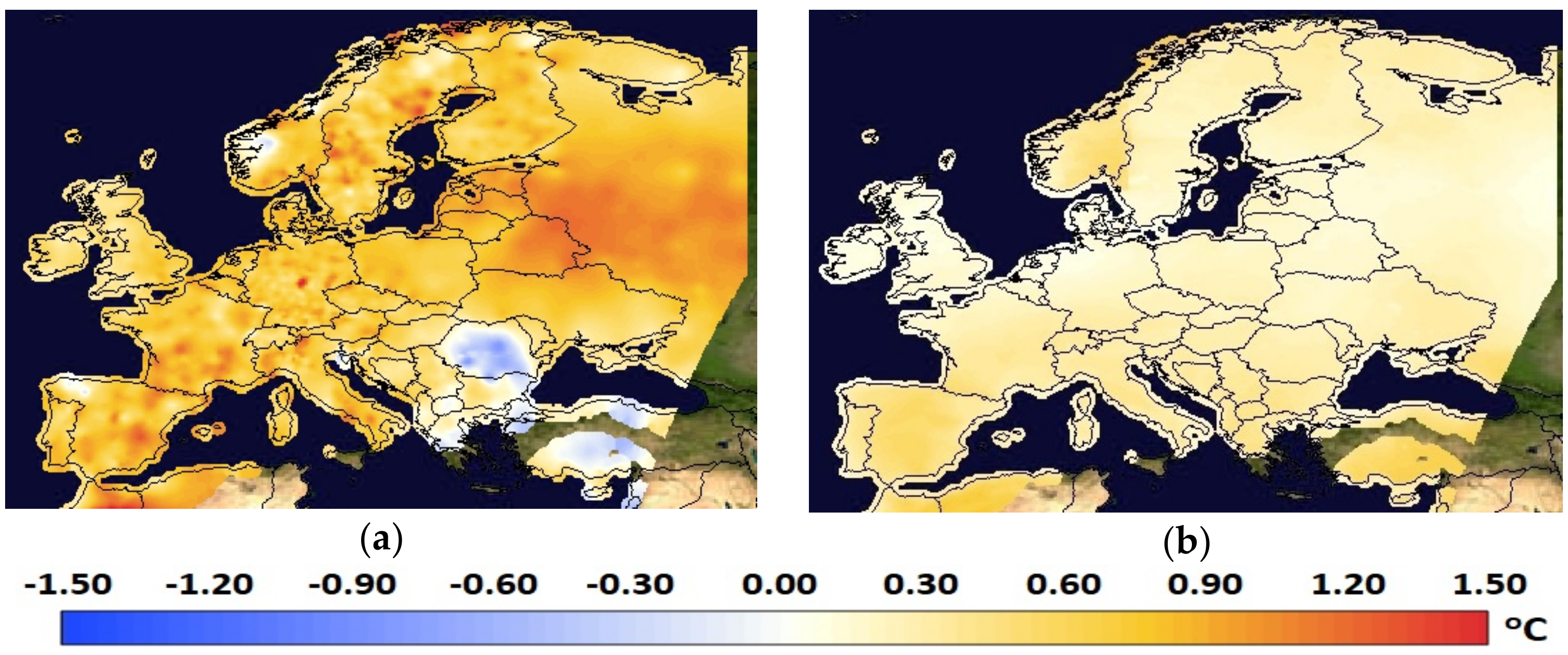
3.1.1. Mean Temperature Change and Bias

The model reproduces both the observed climatological patterns and the cycle of mean temperature, capturing all the basic features. This points to the very good representation of all processes governing the climatology of surface temperature by the modelling setup. As observed in Figure 2a, the observed change in mean surface temperature is uniformly positive for the majority of the European domain, except for Southeastern Europe. This is also the case for the simulated change that took place (Figure 2b). The observed change in mean surface temperature is greater, but very close to the simulated one, implying that the forcing fields (i.e., ModelE2 data) are only slightly cooler than the observed (E-OBS) change.
This is also confirmed by the domain mean values of Table 2, which summarizes the observed temperature change between current (1981–2010) and historic (1951–1980) time slices over the entire European domain and regionally, where the 30-year observed mean warming is 0.7 °C while the simulated one is 0.5 °C, leading to a model bias, defined as the difference between observed and modelled values, of 0.2 °C.
With respect to regional accuracy, the model was able to capture reasonably well both the significant characteristics and the magnitude of mean surface temperature change observed. For all subdomains there is a positive bias (underestimation of warming), compared to E-OBS. The largest bias is observed over IP and MD. The magnitude of the bias can be attributed, in large part, to the topographical characteristics of each region and to the uneven station network that characterizes the E-OBS dataset, with a significantly greater number of stations across BI, ME, AL, and SC than in the southern and eastern parts of the domain.
Seasonally, we obtain a more detailed view concerning the model’s simulation capabilities. Beginning with spring, a warming is observed over most of the domain, except the regions of Romania and Turkey (Figure 3a, left panel). The domain mean warming is 0.9 °C, the largest seen among all seasons, for the examined periods. The surface temperature increase intensifies as we move to the northern–northeastern part of the domain, where a maximum increase of 1.4 °C is observed. The model reproduces the observed during spring surface temperature changes. The simulated bias (Figure 3a, right panel) is negative at the north, pointing to a slight temperature change overestimation by the model, and turns positive at the southern part of Europe (slight temperature change underestimation). The bias though is rather small for all subregions considered ranging between 0.0 for ME and SC and 0.4 for MD (Table 3), while the simulated mean domain bias is 0.1 °C.
Summer observed change (Figure 3b, left panel) has negative to zero values at the far north while being positive for the rest of the map, apart from Romania and the eastern shores of the Mediterranean. Temperature change becomes more significant moving from the east to the west. Model simulated summer temperature change has a similar spatial pattern, as can be inferred form the bias presented (Figure 3b, right panel). The bias is positive all over the domain, having higher values in the west–southwest, and much smaller values from middle east–east end and the northern part. Summer average domain increase was 0.6 °C, while the simulated bias was 0.3 °C (Table 3). The largest underestimation of temperature increase is observed over IP and FR (Table 3). The general tendency of the model towards lower temperatures during summer compared to E-OBS could be attributed to the combination of the NOAH LSM with the RRTMG radiation scheme.
Autumn observed a mean temperature change between the two time slices exhibiting the lowest values among the seasons, with an intense decrease over Romania (Figure 3c, left panel) up to −1 °C. Spatially, the model combination reproduced the observed changes (Figure 3c, right panel) over all subregions (Table 3), exhibiting excellent closure. The average domain warming for this season was 0.4 °C, whereas the model presented a positive bias of 0.1 °C to the simulated one.
Winter actual change (Figure 3d, left panel) presents a similar spatial pattern to spring, with greater values observed over the northeast part of the domain and a decrease over the Balkan-Turkey region. The domain average observed warming is 0.8 °C, close to the spring average warming. Simulated bias (Figure 3d, right panel) is larger at the northern part of the domain and decreases as toward the south. It should be highlighted that the regions characterized by the largest degree of winter bias are SC and EE, coinciding in space with the regions presenting the largest spread in temperature change. This finding is also confirmed by other studies [45]. This spatial pattern of increased bias over the Alps and Northeastern Europe has also been documented in WRF climate forecasts of winter temperature (e.g., [45,65]). This behavior is attributed to the role of snow cover in cooling the surface via snow albedo and snow emissivity feedbacks [8], and the issues of WRF to address surface temperature in snow-covered areas by overestimating surface albedo [72,73].
It is clear from the analysis presented previously that the model consistently underpredicts the temperature change variations observed across all subregions. This indicates that a colder climatology introduced by the employed forcing fields has been assessed, both in terms of seasonal averages and when comparing the entire length of current to historic data. Except for IP, which has its strongest bias during summer, and EE, which has its largest bias during autumn, the bulk of the subregions have their biases at their peak during winter. Among all subregions, the highest bias is found over AL and MD, which is largely caused by the land–atmosphere interactions. Contrarily, with respect to the smallest biases, they are noted either in spring (FR, SC, EE) or in autumn (BI, ME AL, MD). This behavior is driven by the combined effect of the lower snow cover during these seasons compared to winter that counterbalances the overestimation of surface albedo observed during winter, and the milder effect of the radiation scheme as opposed to summer.

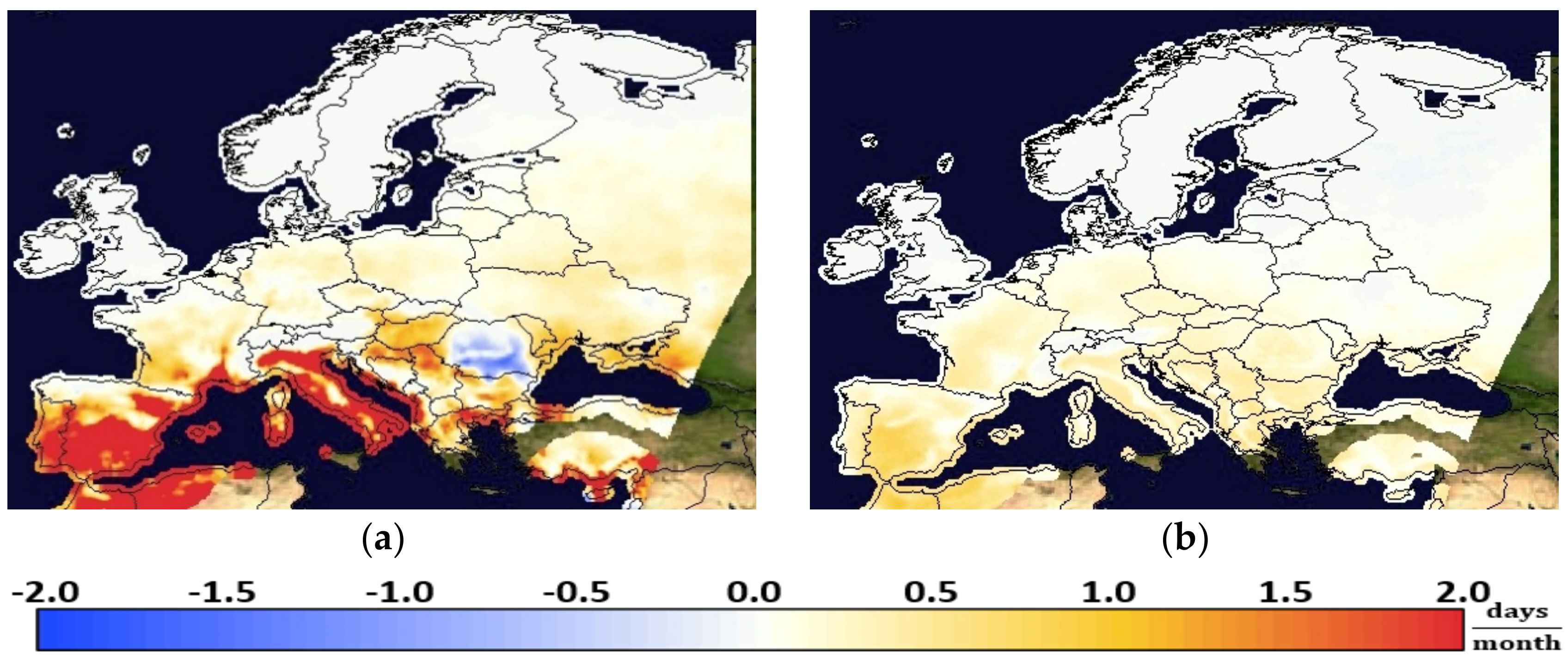
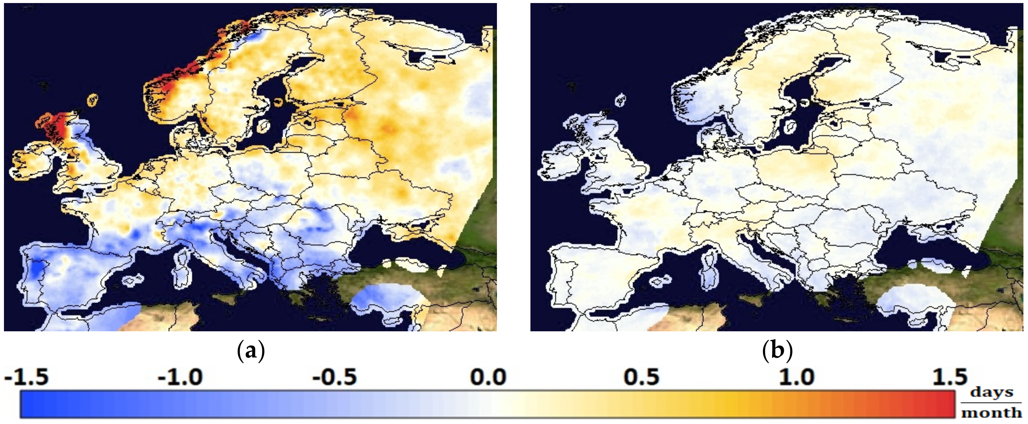
3.1.2. Days Per Month with Mean Temperature over 25 °C

Figure 4 depicts the observed (E-OBS) shift in the number of days for summer (Figure 4a) that temperature exceeded 25 °C and the corresponding model bias (Figure 4b) between current and historic years. During winter, spring, and autumn, the observed and simulated magnitudes of the changes were nearly zero and are not presented here.
When observing the total 30-year mean change during summer, it is evident that both datasets demonstrate a shift toward a greater number of warm days across the vast bulk of southern Europe. The change declines to zero as we proceed north, with insignificant negative values for the simulated change over Romania. The model underestimates the number of days in most subregions examined, except for SC, AL, and BI, wherein the results of the model highly correlate with the data.
Regionally, IP and MD have had the greatest increase in the number of days with mean daily temperatures over 25 °C (9 days per summer season or year compared to the historic average). The model bias is 2 days/year for IP while for MD it is 1 day/year. Over AL an increase of 3 days/year is both observed and simulated. Milder changes were observed over FR (1 day/year), ME (1 day/year), and EE (1 day/year). In each of these instances, a bias of 1 day/year is observed. BI and SC, despite experiencing a warming, did not exceed the threshold temperature, as is also the case for the model’s estimation. NOAH LSM and RRTMG radiation schemes may have contributed to the model’s trend toward lower summer temperatures than E-OBS.

3.2. Precipitation

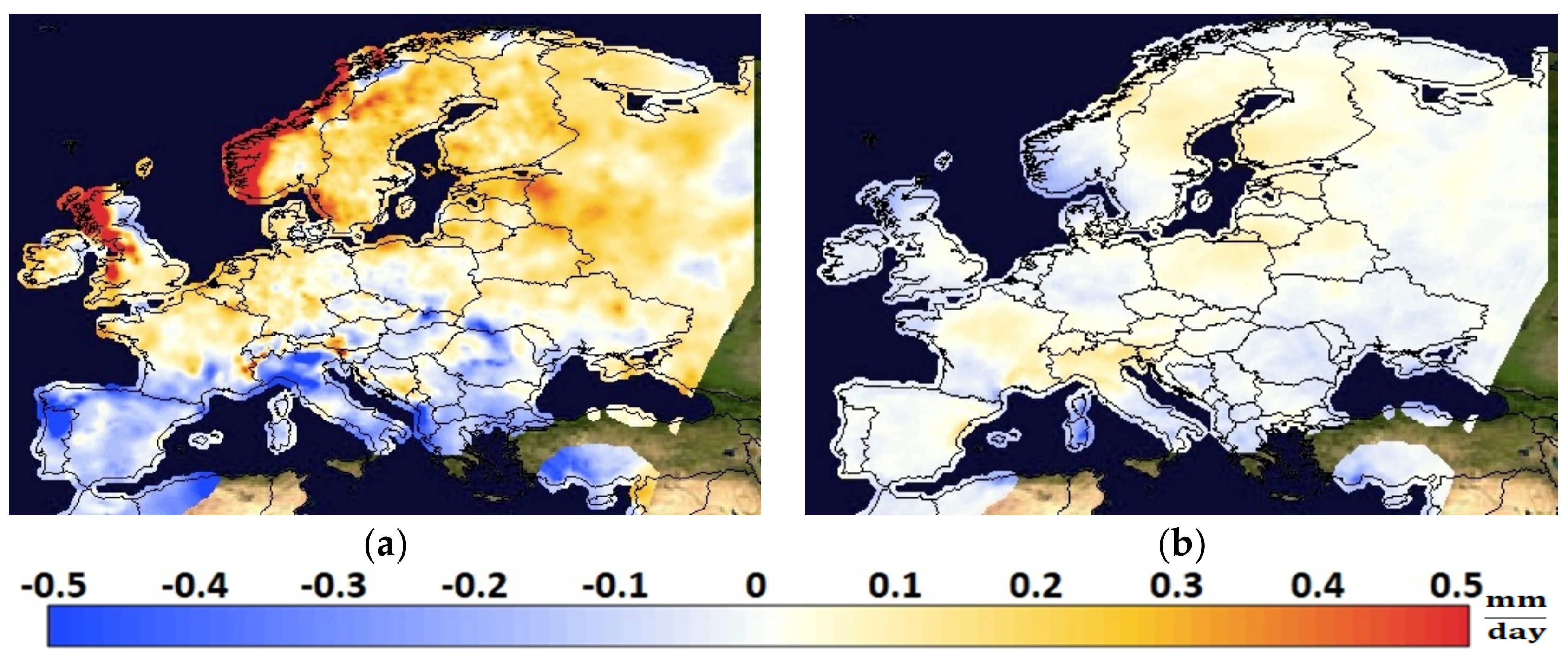
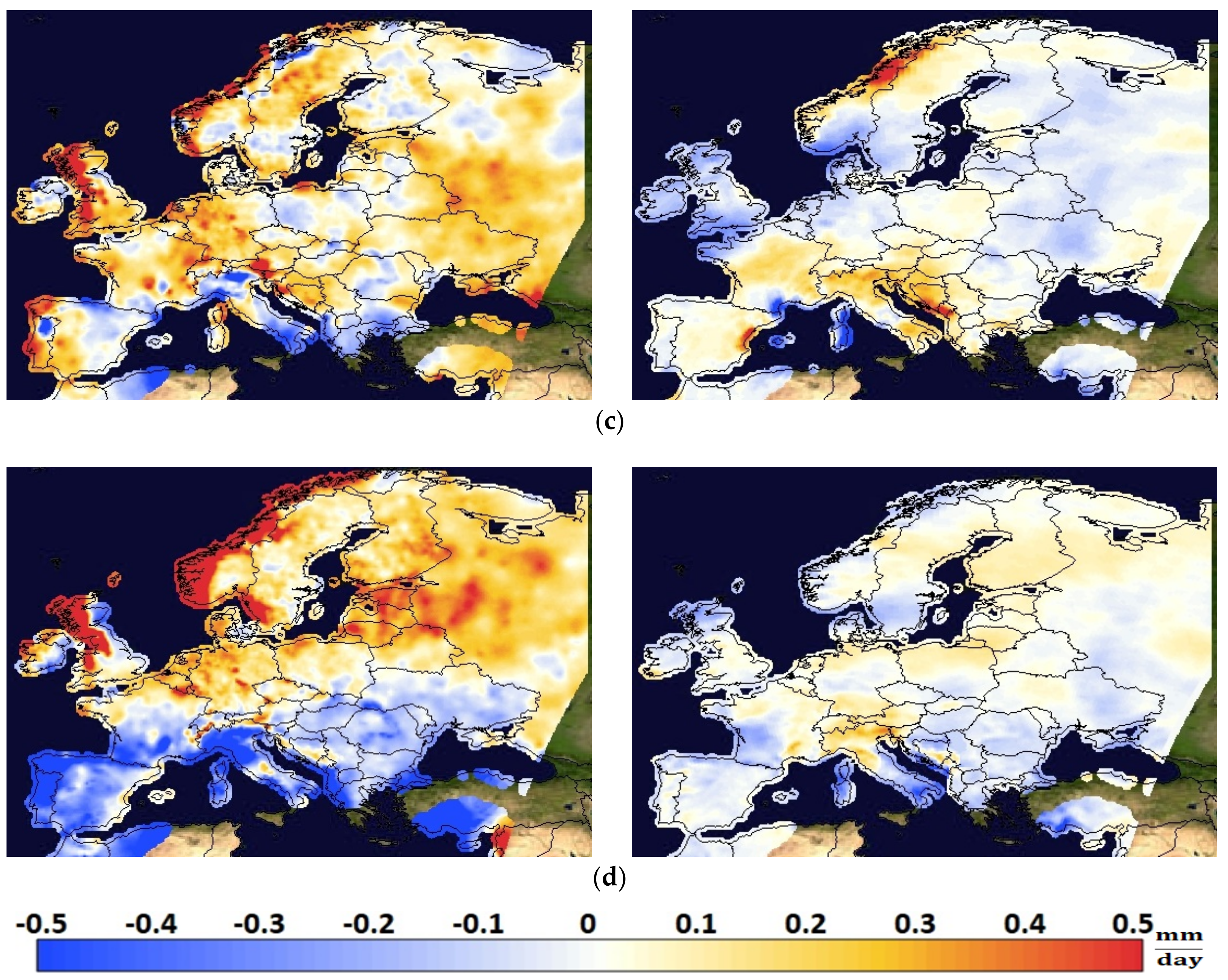
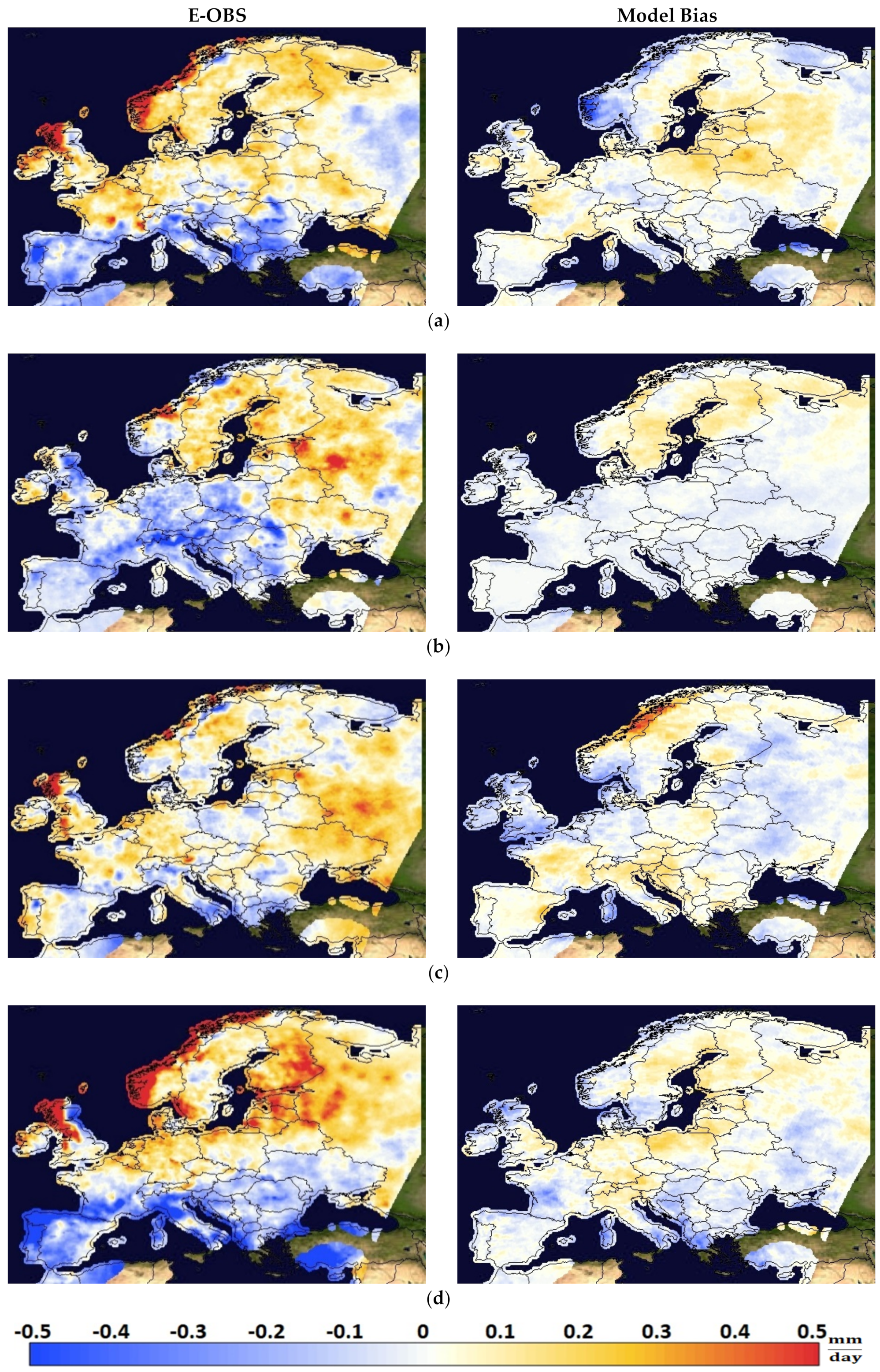
3.2.1. Mean Precipitation

Mean daily precipitation change observed (Figure 5 and Figure 6, left panels) presents a north–south gradient, both when comparing current with historic years and on a seasonal basis of current and historic years. Average rainfall in southern Europe and around the Mediterranean has been decreasing over the study period. Conversely, an increase of up to 0.5 mm in daily precipitation is seen over the northern part of the domain. On average, a domain-wide increase of 0.1 mm/day between current and historic years was observed (Table 4 and Table 5), both annually and seasonally, except in summer, when no change was observed. The transition from the positive to the negative values depends on the season, except in autumn, during which a mixed trend is found. Regionally, BI and SC received the greatest rise in daily precipitation (0.2 mm/day, Table 4), while IP and MD experienced the greatest reduction (−0.2 mm/day, Table 4) when comparing the two periods.
The model captures all the climatological properties of precipitation, as can be concluded from the estimated biases (E-OBS-model) presented (Figure 5 and Figure 6, right panels). The change in mean precipitation simulated by the models closely matches the observed values, both domain-wide and regionally.
Addressing the variable per season, during spring, the average precipitation presents a trend of reduction in the south and an increase to the north, except for the far east area of the map (Russia) (Figure 6). The spring average observed domain increase was 0.1 mm/day (Table 5), equal to the simulated change. The model accurately generated the spatial features of precipitation change observed except over the southeastern part of SC (Norway) and over the northern part of EE where it underestimates the change; conversely, over the northwestern part of SC, the model overestimates it. However, these incremental biases cancel each other out, thus a total bias of 0.0 for SC is estimated. This behavior can be attributed to the convective scheme employed that generated excess precipitation over the mountainous region of Norway, followed by lower precipitation changes to the east. A similar behavior has been reported by other studies as well over mountainous regions [45,74,75], but for the summer season.
During summer, a significant reduction in precipitation has taken place, not only in the south but also in the greater part of central Europe. Conversely, EE and SC faced a notable increase in precipitation (Figure 6b, left panel). Modelling results are comparable with observations. A small overestimation is noted for most of the European domain, except for SC, in which an underestimation is noted (Figure 6b, right panel). In terms of intensity, the model evidently projects a change of similar magnitude with the observation for the entire domain. The summer domain average change was 0.0 mm/day, pointing to a redistribution of precipitation over Europe for summer (Table 5).
In autumn, most of the coastal areas of the Mediterranean experienced a decrease in precipitation, but a consistent north– south gradient pattern is not observed. Continental Europe experienced an increase, more intensely in its central part, Portugal, and Britain (Figure 6c, left panel). The model simulated the changes well, presenting a positive bias over the central part of FR, AL, and part of MD, and a negative bias over BI (Figure 6c, right panel). Summer domain average increase was 0.1 mm/day, while the related simulated bias was 0.0 mm/day.
During winter, the largest changes between current and historic years are observed. Specifically, the winter observed change in average precipitation, indicating a significant decrease across southern Europe, with the highest values among all seasons. There was also a significant increase in the north, with BI and northern SC witnessing the greatest increases in precipitation (Figure 6d, left panel). The changes simulated by the model captured the observed patterns (Figure 6d, right panel). The actual domain average increase was 0.1 mm/day, with the related model bias being 0.0 mm/day. The largest positive bias is noted over AL (Table 5), and the largest negative over MD.
From the analysis performed above, it becomes apparent that the positive or negative model biases do not present a regionally systematic pattern. Nevertheless, a negative bias is observed in most cases, independent of subregion examined. This is a known problem of WRF simulations and has been reported in several studies, particularly when the combination of KF and YSU schemes is employed [73,76]. Some discrepancies also arise from the topographic characteristics of each region that formulate regional weather patterns, indicating an important underlying reason for the deviations assessed.

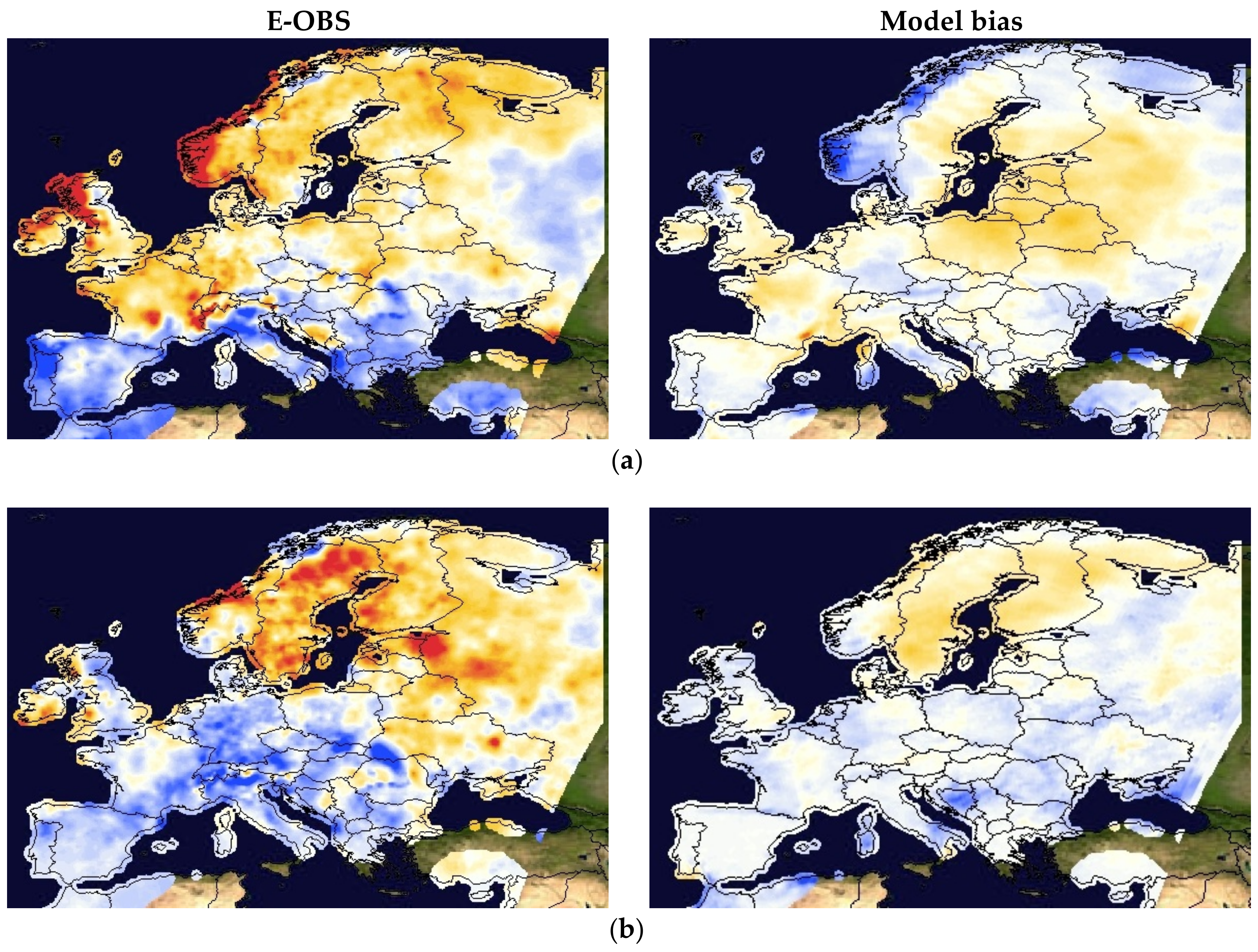
3.2.2. Days Per Month with Mean Daily Precipitation above 5 mm

The number of days per month when the mean daily precipitation exceeded the 5 mm threshold is the final variable examined in this study. This threshold represents a moderate but non-ignorable amount of precipitation. Observing the average observed change that took place between the two 30-year periods (Figure 7a), there is a decrease in the number of days for the central and southern parts of the domain, whereas an increase can be observed in northern FR, ME, and the greater parts of BI and SC. Model simulated bias, depicted in Figure 7b, indicates an insignificant deviation from observations everywhere, revealing a significant skill in estimating changes above the targeted threshold. Domain-wide, an increase of 2 days/year was observed. Regionally, there are regions that faced a more intense change; SC faced the largest increase (6 days/year) followed by BI (5 days/year). Milder was the increase over ME (2 days/year). Conversely, IP experienced the sharpest decrease in the number of days with precipitation greater than 5 mm (6 days/year), followed by MD (5 days/year) and AL (4 days/year).
On a seasonal basis, the change that occurred throughout springs (Figure 8a, left panel) closely resembles the mean change observed between current and historic periods. The shift zone between the positive and the negative change over the European domain is a bit lower in spring compared to the annual one. Small differences are also located at the northeastern part of the map. Comparing the average spring seasons’ modification between current and historic years, regionally, the number of days with precipitation exceeding the 5 mm threshold increased the most in BI (2 days) followed by SC (1 day), FR (1 day) and ME (1 day). In contrast, in IP there was a drop (2 days) in the number of days with precipitation above the threshold; similar was the case for MD (1 day). The remaining subregions exhibited an unimportant fluctuation (0 days), although locally variations may exist. The model bias (Figure 8a, right panel) is 0 days/month everywhere, except EE, where it estimates 1 day less change. Over SC, despite overestimating the change over Norway and underestimating it over the remainder of the subregion, it provides a bias of 0 days/year, replicating the behavior observed for mean precipitation in the 2–30-year comparison. For the rest of the subregions, the bias ranges between 0 and 1 day/year.
As per summer, in every subregion, the number of days with mean daily precipitation of more than 5 mm has declined (Figure 8b, left panel), except for SC, which has seen an increase of 1 day. The most significant shift has occurred in AL, resulting in a total loss of 2 days as compared to the average of the historic summers. The decline is not significant in IP, FR, ME, or MD (all subregions demonstrated a 1-day drop). There was a marginal rise in some areas of BI, but the index did not experience any changes generally. The bias of the model is displayed in the right panel of Figure 8b. Although the bias is characterized by small regional fluctuations, in total, a bias of zero is estimated for all subregions, with a profound trend of slight overestimation everywhere, except for most parts of SC.
Along the same lines as the observed change in the mean amount of precipitation, autumn does not display any particular spatial pattern (Figure 8c, left panel). According to the observations, most of the Mediterranean’s coastal regions are experiencing a decline, but southern Turkey, central Italy, Portugal, and Croatia are experiencing some occasional increases. A significant increase has occurred in the eastern part of the domain. The observations indicate that there is currently a 1-day increase over BI, IP, FR, ME, and SC in comparison to historical years. Conversely, there has been a decrease of 1 day over MD. Absence of change was observed in all other subregions. The model did a reasonably good job of replicating the changes; however, it overestimated the modification over BI by 1 day and equally underestimated it over AL. Once again, the greatest regional heterogeneity is demonstrated in SC, although the observed variations cancel each other out. The observed rise in mean domain values of change was 1 day, which coincides in magnitude with the model’s assessment.
This variable’s observed winter change (Figure 8d, left panel) demonstrates a geographic pattern that is extremely close to its mean change; nevertheless, the transition zone from positive to negative values is moved a bit further north. Both winter increase and decrease of this variable demonstrate the highest values among all seasons, yet the overall change throughout the domain is zero. IP, AL, and MD recorded the highest drop in the number of days above the threshold (3, 2, and 2 days, respectively), whereas BI and SC underwent the largest increase (2 days). The changes that were simulated by the model are comparable to the changes that were observed, exhibiting a bias of zero in the majority of subregions with the exception of ME and AL, where an underestimation of 1 day is found, and MD, where an overestimation of 1 day is assessed.

4. Discussion and Conclusions

In this study, the ability of a combination of GCM-RCM models, namely NASA Goddard Institute for Space Studies (GISS) GCM ModelE2 and WRFv4.0 ARW to replicate the observed bias and temporal variability and reproduce the impact of climate change on critical meteorological parameters that has already occurred was evaluated. The European domain was selected for this exercise. Examining the accuracy with which a model replicates changes in climatic factors that have occurred over the course of the last several decades is an intriguing task, given that RCM outputs are still susceptible to climate model errors originating from the structure of the RCM itself, and from the initial and boundary conditions provided by the driving GCM/ESM. Nonetheless, this exercise enables the identification of regions where systematic biases exist and the examination of the underlying causes for this. A 60-year period was selected from 1951–2010, with the first half representing the historic time slice and the latter the current time slice. Modeling biases for mean temperature, mean precipitation, number of days that temperature exceeded 25 °C, and number of days that precipitation exceeded the threshold of 5 mm, according to the WMO guidelines, were compared against observations from E-OBS at a spatial resolution of 0.25°.
The analysis performed above makes it abundantly evident that the model underpredicts the mean temperature changes found across all subregions consistently. This implies that a colder climatology has been assessed, both with respect to seasonal averages and when comparing the overall length of current to historic data, underlying the importance of the driving model. Except for IP, for which the greatest bias is observed during summer, and EE, for which the highest bias is noted during autumn, for most of the subregions the greatest bias is simulated during winter. From them, the southern and eastern subregions indicate the most bias when compared to the remainder of the areas, owing to interactions between the land and the atmosphere. The smallest biases, conversely, are simulated either in spring (FR, SC, EE) or in autumn (BI, ME, AL, MD). This tendency is mostly related to the combined effect of the decreased snow cover throughout these seasons compared to winter, which offsets the overestimation of surface albedo seen during winter, and the softer influence of the radiation scheme as opposed to summer.
Most of Southern Europe experiences an increase in the number of warm days (days in which mean temperature exceeds 25 °C) during the summer months only. In most subregions examined, the model underestimates the number of days, except for SC, AL, and BI, where the model’s results closely match the data. The number of warm days has increased the most in IP and MD (9 days/year) with an associated model bias of 2 days/year for IP, and 1 day/year for MD. A rise of 3 days/year is observed and modelled over AL. Milder alterations of 1 day/year were found in FR, ME, and EE with the model bias being about 1 day/year. BI and SC did not surpass the temperature threshold, as does the model’s assessment. NOAH LSM and RRTMG radiation schemes may have contributed to the model’s trend toward lower summer temperatures more than E-OBS.
With respect to mean precipitation, the positive or negative model biases do not indicate a regionally regular trend. Regardless of the subregion studied, a negative bias is indicated in most cases. This is a well known issue in WRF simulations and has been observed in various studies, particularly when the KF and YSU schemes are used. Some inconsistencies are also caused by the geographic characteristics of each region, which shape regional weather patterns, implying an essential underlying cause for the variations observed.
With respect to the number of days per month that mean daily precipitation surpassed 5 mm, over the two time slices examined, the central and southern regions of the domain saw fewer days, while northern FR, ME, and large parts of BI and SC saw more. The model simulated bias is very small everywhere, indicating skill in estimating changes over the specified threshold. Similarly, on a seasonal basis, model results were in all instances comparable with observations, although unimportant regional variations may exist.
The results of this study were obtained focusing solely on two parameters, i.e., temperature and precipitation. Further analysis incorporating parameters such as the cloud properties and SSTs is left for a future study. Nonetheless, the preceding exercise emphasizes both the significance and the need for further observations, particularly from the southern regions of the European domain, for more reliable evaluation studies.

Author Contributions

Conceptualization, I.S., E.T. and R.-E.P.S.; methodology, I.S., E.T. and R.-E.P.S.; software, I.S.; validation, I.S.; formal analysis, E.T. and R.-E.P.S.; investigation, I.S., E.T. and R.-E.P.S.; resources, E.T. and R.-E.P.S.; data curation, I.S.; writing—original draft preparation, I.S.; writing—review and editing, E.T. and R.-E.P.S.; visualization, I.S.; supervision, R.-E.P.S.; project administration, R.-E.P.S. All authors have read and agreed to the published version of the manuscript.

Funding

This research received no external funding.

Institutional Review Board Statement

Not applicable.

Informed Consent Statement

Not applicable.

Data Availability Statement

Not applicable.

Acknowledgments

This work was supported by the EU LIFE CLIMATREE project “A novel approach for accounting & monitoring carbon sequestration of tree crops and their potential as carbon sink areas” (LIFE14 CCM/GR/000635). We acknowledge the E-OBS dataset from the EU-FP6 project ENSEMBLES (http://ensembles-eu.metoffice.com, accessed on 16 June 2022) and the data providers in the ECA&D project (http://www.ecad.eu, accessed on 16 June 2022).

Conflicts of Interest

The authors declare no conflict of interest.

References

  1. Masson-Delmotte, V.; Zhai, P.; Pirani, A.; Connors, S.L.; Péan, C.; Berger, S.; Caud, N.; Chen, Y.; Goldfarb, L.; Gomis, M.I.; et al. (Eds.) IPCC, 2021: Climate Change 2021: The Physical Science Basis. Contribution of Working Group I to the Sixth Assessment Report of the Intergovernmental Panel on Climate Change; Cambridge University Press: Cambridge, UK; New York, NY, USA, 2021; in press. [Google Scholar] [CrossRef]
  2. Giorgi, F.; Gutowski, W.J. Coordinated Experiments for Projections of Regional Climate Change. Curr. Clim. Change Rep. 2016, 2, 202–210. [Google Scholar] [CrossRef] [Green Version]
  3. Knutti, R.; Sedláček, J. Robustness and Uncertainties in the New CMIP5 Climate Model Projections. Nat. Clim. Chang. 2013, 3, 369–373. [Google Scholar] [CrossRef]
  4. Christensen, J.H.; Carter, T.R.; Rummukainen, M.; Amanatidis, G. Evaluating the Performance and Utility of Regional Climate Models: The PRUDENCE Project. Clim. Chang. 2007, 81, 1–6. [Google Scholar] [CrossRef]
  5. Beniston, M.; Goyette, S. Changes in Variability and Persistence of Climate in Switzerland: Exploring 20th Century Observations and 21st Century Simulations. Glob. Planet. Chang. 2007, 57, 1–15. [Google Scholar] [CrossRef] [Green Version]
  6. Christensen, J.H.; Carter, T.R.; Giorgi, F. PRUDENCE Employs New Methods to Assess European Climate Change. Eos Trans. Am. Geophys. Union 2002, 83, 147. [Google Scholar] [CrossRef]
  7. Christensen, J.H.; Christensen, O.B. A Summary of the PRUDENCE Model Projections of Changes in European Climate by the End of This Century. Clim. Chang. 2007, 81, 7–30. [Google Scholar] [CrossRef]
  8. Déqué, M.; Rowell, D.P.; Lüthi, D.; Giorgi, F.; Christensen, J.H.; Rockel, B.; Jacob, D.; Kjellström, E.; de Castro, M.; van den Hurk, B. An Intercomparison of Regional Climate Simulations for Europe: Assessing Uncertainties in Model Projections. Clim. Chang. 2007, 81, 53–70. [Google Scholar] [CrossRef]
  9. ENSEMBLES: Climate Change and Its Impacts: Summary of Research and Results from the ENSEMBLES Project—European Environment Agency. Available online: https://www.eea.europa.eu/data-and-maps/indicators/global-and-european-temperature-1/ensembles-climate-change-and-its (accessed on 9 July 2022).
  10. Doblas-Reyes, F.J.; Weisheimer, A.; Déqué, M.; Keenlyside, N.; McVean, M.; Murphy, J.M.; Rogel, P.; Smith, D.; Palmer, T.N. Addressing Model Uncertainty in Seasonal and Annual Dynamical Ensemble Forecasts. Q. J. R. Meteorol. Soc. 2009, 135, 1538–1559. [Google Scholar] [CrossRef] [Green Version]
  11. Weisheimer, A.; Doblas-Reyes, F.J.; Palmer, T.N.; Alessandri, A.; Arribas, A.; Déqué, M.; Keenlyside, N.; MacVean, M.; Navarra, A.; Rogel, P. ENSEMBLES: A New Multi-Model Ensemble for Seasonal-to-Annual Predictions—Skill and Progress beyond DEMETER in Forecasting Tropical Pacific SSTs. Geophys. Res. Lett. 2009, 36, L21711. [Google Scholar] [CrossRef] [Green Version]
  12. Jacob, D.; Bärring, L.; Christensen, O.B.; Christensen, J.H.; de Castro, M.; Déqué, M.; Giorgi, F.; Hagemann, S.; Hirschi, M.; Jones, R.; et al. An Inter-Comparison of Regional Climate Models for Europe: Model Performance in Present-Day Climate. Clim. Chang. 2007, 81, 31–52. [Google Scholar] [CrossRef]
  13. Kotlarski, S.; Keuler, K.; Christensen, O.B.; Colette, A.; Déqué, M.; Gobiet, A.; Goergen, K.; Jacob, D.; Lüthi, D.; Van Meijgaard, E.; et al. Regional Climate Modeling on European Scales: A Joint Standard Evaluation of the EURO-CORDEX RCM Ensemble. Geosci. Model Dev. 2014, 7, 1297–1333. [Google Scholar] [CrossRef] [Green Version]
  14. Jacob, D.; Petersen, J.; Eggert, B.; Alias, A.; Christensen, O.B.; Bouwer, L.M.; Braun, A.; Colette, A.; Déqué, M.; Georgievski, G.; et al. EURO-CORDEX: New High-Resolution Climate Change Projections for European Impact Research. Reg. Environ. Chang. 2014, 14, 563–578. [Google Scholar] [CrossRef]
  15. Ruti, P.M.; Somot, S.; Giorgi, F.; Dubois, C.; Flaounas, E.; Obermann, A.; Dell’Aquila, A.; Pisacane, G.; Harzallah, A.; Lombardi, E.; et al. Med-CORDEX Initiative for Mediterranean Climate Studies. Bull. Am. Meteorol. Soc. 2016, 97, 1187–1208. [Google Scholar] [CrossRef] [Green Version]
  16. Kjellström, E.; Boberg, F.; Castro, M.; Christensen, J.H.; Nikulin, G.; Sánchez, E. Daily and Monthly Temperature and Precipitation Statistics as Performance Indicators for Regional Climate Models. Clim. Res. 2010, 44, 135–150. [Google Scholar] [CrossRef]
  17. Lenderink, G. Exploring Metrics of Extreme Daily Precipitation in a Large Ensemble of Regional Climate Model Simulations. Clim. Res. 2010, 44, 151–166. [Google Scholar] [CrossRef]
  18. Lorenz, P.; Jacob, D. Validation of Temperature Trends in the ENSEMBLES Regional Climate Model Runs Driven by ERA40. Clim. Res. 2010, 44, 167–177. [Google Scholar] [CrossRef]
  19. Sanchez-Gomez, E.; Somot, S.; Déqué, M. Ability of an Ensemble of Regional Climate Models to Reproduce Weather Regimes over Europe-Atlantic during the Period 1961–2000. Clim. Dyn. 2009, 33, 723–736. [Google Scholar] [CrossRef]
  20. Sanchez-Gomez, E.; Somot, S.; Josey, S.A.; Dubois, C.; Elguindi, N.; Déqué, M. Evaluation of Mediterranean Sea Water and Heat Budgets Simulated by an Ensemble of High Resolution Regional Climate Models. Clim. Dyn. 2011, 37, 2067–2086. [Google Scholar] [CrossRef] [Green Version]
  21. Vautard, R.; Gobiet, A.; Jacob, D.; Belda, M.; Colette, A.; Déqué, M.; Fernández, J.; García-Díez, M.; Goergen, K.; Güttler, I.; et al. The Simulation of European Heat Waves from an Ensemble of Regional Climate Models within the EURO-CORDEX Project. Clim. Dyn. 2013, 41, 2555–2575. [Google Scholar] [CrossRef]
  22. Aalbers, E.E.; Lenderink, G.; van Meijgaard, E.; van den Hurk, B.J.J.M. Local-Scale Changes in Mean and Heavy Precipitation in Western Europe, Climate Change or Internal Variability? Clim. Dyn. 2018, 50, 4745–4766. [Google Scholar] [CrossRef] [Green Version]
  23. Christensen, O.B.; Kjellström, E. Partitioning Uncertainty Components of Mean Climate and Climate Change in a Large Ensemble of European Regional Climate Model Projections. Clim. Dyn. 2020, 54, 4293–4308. [Google Scholar] [CrossRef]
  24. Vautard, R.; Kadygrov, N.; Iles, C.; Boberg, F.; Buonomo, E.; Bülow, K.; Coppola, E.; Corre, L.; van Meijgaard, E.; Nogherotto, R.; et al. Evaluation of the Large EURO-CORDEX Regional Climate Model Ensemble. J. Geophys. Res. Atmos. 2021, 126, e2019JD032344. [Google Scholar] [CrossRef]
  25. Kendon, E.J.; Jones, R.G.; Kjellström, E.; Murphy, J.M. Using and Designing GCM–RCM Ensemble Regional Climate Projections. J. Clim. 2010, 23, 6485–6503. [Google Scholar] [CrossRef]
  26. Sørland, S.L.; Schär, C.; Lüthi, D.; Kjellström, E. Bias Patterns and Climate Change Signals in GCM-RCM Model Chains. Environ. Res. Lett. 2018, 13, 074017. [Google Scholar] [CrossRef]
  27. Wilby, R.L.; Wigley, T.M.L. Downscaling General Circulation Model Output: A Review of Methods and Limitations. Prog. Phys. Geogr. Earth Environ. 1997, 21, 530–548. [Google Scholar] [CrossRef]
  28. Maraun, D. Bias Correction, Quantile Mapping, and Downscaling: Revisiting the Inflation Issue. J. Clim. 2013, 26, 2137–2143. [Google Scholar] [CrossRef] [Green Version]
  29. Russell, G.L.; Miller, J.R.; Rind, D. A Coupled Atmosphere-ocean Model for Transient Climate Change Studies. Atmos.-Ocean 1995, 33, 683–730. [Google Scholar] [CrossRef]
  30. Hansen, J.; Sato, M.; Ruedy, R.; Kharecha, P.; Lacis, A.; Miller, R.; Nazarenko, L.; Lo, K.; Schmidt, G.A.; Russell, G.; et al. Climate Simulations for 1880–2003 with GISS ModelE. Clim. Dyn. 2007, 29, 661–696. [Google Scholar] [CrossRef] [Green Version]
  31. Schmidt, G.A.; Ruedy, R.; Hansen, J.E.; Aleinov, I.; Bell, N.; Bauer, M.; Bauer, S.; Cairns, B.; Canuto, V.; Cheng, Y.; et al. Present-Day Atmospheric Simulations Using GISS ModelE: Comparison to In Situ, Satellite, and Reanalysis Data. J. Clim. 2006, 19, 153–192. [Google Scholar] [CrossRef]
  32. Miller, R.L.; Schmidt, G.A.; Nazarenko, L.S.; Tausnev, N.; Bauer, S.E.; DelGenio, A.D.; Kelley, M.; Lo, K.K.; Ruedy, R.; Shindell, D.T.; et al. CMIP5 Historical Simulations (1850–2012) with GISS ModelE2. J. Adv. Model. Earth Syst. 2014, 6, 441–478. [Google Scholar] [CrossRef]
  33. Schmidt, G.A.; Kelley, M.; Nazarenko, L.; Ruedy, R.; Russell, G.L.; Aleinov, I.; Bauer, M.; Bauer, S.E.; Bhat, M.K.; Bleck, R.; et al. Configuration and Assessment of the GISS ModelE2 Contributions to the CMIP5 Archive. J. Adv. Model. Earth Syst. 2014, 6, 141–184. [Google Scholar] [CrossRef]
  34. Nazarenko, L.; Schmidt, G.A.; Miller, R.L.; Tausnev, N.; Kelley, M.; Ruedy, R.; Russell, G.L.; Aleinov, I.; Bauer, M.; Bauer, S.; et al. Future Climate Change under RCP Emission Scenarios with GISS ModelE2. J. Adv. Model. Earth Syst. 2015, 7, 244–267. [Google Scholar] [CrossRef] [Green Version]
  35. Kim, Y.; Moorcroft, P.R.; Aleinov, I.; Puma, M.J.; Kiang, N.Y. Variability of Phenology and Fluxes of Water and Carbon with Observed and Simulated Soil Moisture in the Ent Terrestrial Biosphere Model (Ent TBM Version 1.0.1.0.0). Geosci. Model Dev. 2015, 8, 3837–3865. [Google Scholar] [CrossRef] [Green Version]
  36. Del Genio, A.D.; Yao, M.-S. Efficient Cumulus Parameterization for Long-Term Climate Studies: The GISS Scheme. In The Representation of Cumulus Convection in Numerical Models; Emanuel, K.A., Raymond, D.J., Eds.; American Meteorological Society: Boston, MA, USA, 1993; pp. 181–184. ISBN 978-1-935704-13-3. [Google Scholar]
  37. Del Genio, A.D.; Yao, M.-S.; Kovari, W.; Lo, K.K.-W. A Prognostic Cloud Water Parameterization for Global Climate Models. J. Clim. 1996, 9, 270–304. [Google Scholar] [CrossRef] [Green Version]
  38. Kim, D.; Sobel, A.H.; Del Genio, A.D.; Chen, Y.; Camargo, S.J.; Yao, M.-S.; Kelley, M.; Nazarenko, L. The Tropical Subseasonal Variability Simulated in the NASA GISS General Circulation Model. J. Clim. 2012, 25, 4641–4659. [Google Scholar] [CrossRef]
  39. Kim, D.; Del Genio, A.D.; Yao, M.-S. Moist convection scheme in ModelE2, 2011, technical report, NASA Goddard Inst. for Space Stud. arXiv 2013, arXiv:1312.7496. [Google Scholar]
  40. Skamarock, W.C.; Klemp, J.B.; Dudhia, J.; Gill, D.O.; Barker, D.M.; Wang, W.; Powers, J.G. A Description of the Advanced Research WRF Version 3; National Center for Atmospheric Research: Boulder, CO, USA, 2008. [Google Scholar] [CrossRef]
  41. Powers, J.G.; Klemp, J.B.; Skamarock, W.C.; Davis, C.A.; Dudhia, J.; Gill, D.O.; Coen, J.L.; Gochis, D.J.; Ahmadov, R.; Peckham, S.E.; et al. The Weather Research and Forecasting Model: Overview, System Efforts, and Future Directions. Bull. Am. Meteorol. Soc. 2017, 98, 1717–1737. [Google Scholar] [CrossRef]
  42. Skamarock, W.C.; Klemp, J.B.; Dudhia, J.; Gill, D.O.; Liu, Z.; Berner, J.; Wang, W.; Powers, J.G.; Duda, M.G.; Barker, D.M.; et al. A Description of the Advanced Research WRF Model Version 4; National Center for Atmospheric Research: Boulder, CO, USA, 2019. [Google Scholar]
  43. Soares, P.M.M.; Cardoso, R.M.; Miranda, P.M.A.; de Medeiros, J.; Belo-Pereira, M.; Espirito-Santo, F. WRF High Resolution Dynamical Downscaling of ERA-Interim for Portugal. Clim. Dyn. 2012, 39, 2497–2522. [Google Scholar] [CrossRef]
  44. Cardoso, R.M.; Soares, P.M.M.; Miranda, P.M.A.; Belo-Pereira, M. WRF High Resolution Simulation of Iberian Mean and Extreme Precipitation Climate. Int. J. Climatol. 2013, 33, 2591–2608. [Google Scholar] [CrossRef]
  45. Katragkou, E.; Garciá-Diéz, M.; Vautard, R.; Sobolowski, S.; Zanis, P.; Alexandri, G.; Cardoso, R.M.; Colette, A.; Fernandez, J.; Gobiet, A.; et al. Regional Climate Hindcast Simulations within EURO-CORDEX: Evaluation of a WRF Multi-Physics Ensemble. Geosci. Model Dev. 2015, 8, 603–618. [Google Scholar] [CrossRef] [Green Version]
  46. Knist, S.; Goergen, K.; Simmer, C. Evaluation and Projected Changes of Precipitation Statistics in Convection-Permitting WRF Climate Simulations over Central Europe. Clim. Dyn. 2020, 55, 325–341. [Google Scholar] [CrossRef] [Green Version]
  47. Pavlidis, V.; Katragkou, E.; Prein, A.; Georgoulias, A.K.; Kartsios, S.; Zanis, P.; Karacostas, T. Investigating the Sensitivity to Resolving Aerosol Interactions in Downscaling Regional Model Experiments with WRFv3.8.1 over Europe. Geosci. Model Dev. 2020, 13, 2511–2532. [Google Scholar] [CrossRef]
  48. Stergiou, I.; Tagaris, E.; Sotiropoulou, R.-E.P. Investigating the WRF Temperature and Precipitation Performance Sensitivity to Spatial Resolution over Central Europe. Atmosphere 2021, 12, 278. [Google Scholar] [CrossRef]
  49. Jerez, S.; López-Romero, J.M.; Turco, M.; Lorente-Plazas, R.; Gómez-Navarro, J.J.; Jiménez-Guerrero, P.; Montávez, J.P. On the Spin-Up Period in WRF Simulations Over Europe: Trade-Offs Between Length and Seasonality. J. Adv. Model. Earth Syst. 2020, 12, e2019MS001945. [Google Scholar] [CrossRef] [Green Version]
  50. Cornes, R.C.; van der Schrier, G.; van den Besselaar, E.J.; Jones, P.D. An Ensemble Version of the E-OBS Temperature and Precipitation Data Sets. J. Geophys. Res. Atmos. 2018, 123, 9391–9409. [Google Scholar] [CrossRef] [Green Version]
  51. Prein, A.F.; Gobiet, A.; Suklitsch, M.; Truhetz, H.; Awan, N.K.; Keuler, K.; Georgievski, G. Added Value of Convection Permitting Seasonal Simulations. Clim. Dyn. 2013, 41, 2655–2677. [Google Scholar] [CrossRef] [Green Version]
  52. Hofstra, N.; Haylock, M.; New, M.; Jones, P.D. Testing E-OBS European High-Resolution Gridded Data Set of Daily Precipitation and Surface Temperature. J. Geophys. Res. Atmos. 2009, 114, D21101. [Google Scholar] [CrossRef]
  53. Haylock, M.R.; Hofstra, N.; Klein Tank, A.M.G.; Klok, E.J.; Jones, P.D.; New, M. A European Daily High-Resolution Gridded Data Set of Surface Temperature and Precipitation for 1950–2006. J. Geophys. Res. Atmos. 2008, 113, D20119. [Google Scholar] [CrossRef] [Green Version]
  54. Kotlarski, S.; Szabó, P.; Herrera, S.; Räty, O.; Keuler, K.; Soares, P.M.; Cardoso, R.M.; Bosshard, T.; Pagé, C.; Boberg, F.; et al. Observational Uncertainty and Regional Climate Model Evaluation: A Pan-European Perspective. Int. J. Climatol. 2019, 39, 3730–3749. [Google Scholar] [CrossRef] [Green Version]
  55. Cardell, M.F.; Romero, R.; Amengual, A.; Homar, V.; Ramis, C. A Quantile–Quantile Adjustment of the EURO-CORDEX Projections for Temperatures and Precipitation. Int. J. Climatol. 2019, 39, 2901–2918. [Google Scholar] [CrossRef]
  56. Velikou, K.; Tolika, K.; Anagnostopoulou, C.; Zanis, P. Sensitivity Analysis of RegCM4 Model: Present Time Simulations over the Mediterranean. Theor. Appl. Climatol. 2019, 136, 1185–1208. [Google Scholar] [CrossRef]
  57. Min, E.; Hazeleger, W.; Van Oldenborgh, G.J.; Sterl, A. Evaluation of Trends in High Temperature Extremes in North-Western Europe in Regional Climate Models. Environ. Res. Lett. 2013, 8, 014011. [Google Scholar] [CrossRef] [Green Version]
  58. Nikulin, G.; Kjellström, E.; Hansson, U.; Strandberg, G.; Ullerstig, A. Evaluation and Future Projections of Temperature, Precipitation and Wind Extremes over Europe in an Ensemble of Regional Climate Simulations. Tellus A Dyn. Meteorol. Oceanogr. 2011, 63, 41–55. [Google Scholar] [CrossRef] [Green Version]
  59. Bellprat, O.; Kotlarski, S.; Lüthi, D.; Schär, C. Exploring Perturbed Physics Ensembles in a Regional Climate Model. J. Clim. 2012, 25, 4582–4599. [Google Scholar] [CrossRef]
  60. Hofstra, N.; New, M.; McSweeney, C. The Influence of Interpolation and Station Network Density on the Distributions and Trends of Climate Variables in Gridded Daily Data. Clim. Dyn. 2010, 35, 841–858. [Google Scholar] [CrossRef]
  61. Maraun, D.; Osborn, T.J.; Rust, H.W. The Influence of Synoptic Airflow on UK Daily Precipitation Extremes. Part II: Regional Climate Model and E-OBS Data Validation. Clim. Dyn. 2012, 39, 287–301. [Google Scholar] [CrossRef]
  62. Boris, S. Correction of Precipitation Measurements: ETH/IAHS/WMO Workshop on the Correction of Precipitation Measurements, Zurich, 1–3 April 1985; ETH/IAHS/WMO Workshop on the Correction of Precipitation Measurements, Ed.; Geographisches Institut, Eidgenössische Technische Hochschule: Zürich, Switzerland, 1986. [Google Scholar]
  63. Prein, A.F.; Gobiet, A. Impacts of Uncertainties in European Gridded Precipitation Observations on Regional Climate Analysis. Int. J. Climatol. 2017, 37, 305–327. [Google Scholar] [CrossRef]
  64. Schmidt, G.A.; Jungclaus, J.H.; Ammann, C.M.; Bard, E.; Braconnot, P.; Crowley, T.J.; Delaygue, G.; Joos, F.; Krivova, N.A.; Muscheler, R.; et al. Climate Forcing Reconstructions for Use in PMIP Simulations of the Last Millennium (v1.1). Geosci. Model Dev. 2012, 5, 185–191. [Google Scholar] [CrossRef] [Green Version]
  65. Mooney, P.A.; Mulligan, F.J.; Fealy, R. Evaluation of the Sensitivity of the Weather Research and Forecasting Model to Parameterization Schemes for Regional Climates of Europe over the Period 1990–95. J. Clim. 2013, 26, 1002–1017. [Google Scholar] [CrossRef] [Green Version]
  66. Hong, S.-Y.; Dudhia, J.; Chen, S.-H. A Revised Approach to Ice Microphysical Processes for the Bulk Parameterization of Clouds and Precipitation. Mon. Weather Rev. 2004, 132, 103–120. [Google Scholar] [CrossRef]
  67. Iacono, M.J.; Delamere, J.S.; Mlawer, E.J.; Shephard, M.W.; Clough, S.A.; Collins, W.D. Radiative Forcing by Long-Lived Greenhouse Gases: Calculations with the AER Radiative Transfer Models. J. Geophys. Res. Atmos. 2008, 113, D13103. [Google Scholar] [CrossRef]
  68. Hong, S.-Y.; Noh, Y.; Dudhia, J. A New Vertical Diffusion Package with an Explicit Treatment of Entrainment Processes. Mon. Weather Rev. 2006, 134, 2318–2341. [Google Scholar] [CrossRef] [Green Version]
  69. Kain, J.S. The Kain–Fritsch Convective Parameterization: An Update. J. Appl. Meteorol. Climatol. 2004, 43, 170–181. [Google Scholar] [CrossRef] [Green Version]
  70. Chen, F.; Mitchell, K.; Schaake, J.; Xue, Y.; Pan, H.-L.; Koren, V.; Duan, Q.Y.; Ek, M.; Betts, A. Modeling of Land Surface Evaporation by Four Schemes and Comparison with FIFE Observations. J. Geophys. Res. Atmos. 1996, 101, 7251–7268. [Google Scholar] [CrossRef] [Green Version]
  71. WMO. WMO Guidelines on the Calculation of Climate Normals, 2017 edition; WMO: Geneva, Switzerland, 2017; ISBN 978-92-63-11203-3. [Google Scholar]
  72. García-Díez, M.; Fernández, J.; Fita, L.; Yagüe, C. Seasonal Dependence of WRF Model Biases and Sensitivity to PBL Schemes over Europe. Q. J. R. Meteorol. Soc. 2013, 139, 501–514. [Google Scholar] [CrossRef] [Green Version]
  73. García-Díez, M.; Fernández, J.; Vautard, R. An RCM Multi-Physics Ensemble over Europe: Multi-Variable Evaluation to Avoid Error Compensation. Clim. Dyn. 2015, 45, 3141–3156. [Google Scholar] [CrossRef] [Green Version]
  74. Torma, C.; Coppola, E.; Giorgi, F.; Bartholy, J.; Pongrácz, R. Validation of a High-Resolution Version of the Regional Climate Model RegCM3 over the Carpathian Basin. J. Hydrometeorol. 2011, 12, 84–100. [Google Scholar] [CrossRef]
  75. Mystakidis, S.; Zanis, P.; Dogras, C.; Katragkou, E.; Pytharoulis, I.; Melas, D.; Anadranistakis, E.; Feidas, H. Optimization of a Regional Climate Model for High Resolution Simulations over Greece. In Advances in Meteorology, Climatology and Atmospheric Physics; Helmis, C.G., Nastos, P.T., Eds.; Springer: Berlin/Heidelberg, Germany, 2013; pp. 623–629. [Google Scholar]
  76. Evans, J.P.; Ekström, M.; Ji, F. Evaluating the Performance of a WRF Physics Ensemble over South-East Australia. Clim. Dyn. 2012, 39, 1241–1258. [Google Scholar] [CrossRef]
Figure 1. Domain setup (a) WRF model domains at 0.75° and 0.25° grid size resolutions (b) WRF domain map factor, (c) the subregions considered, where 1. BI, 2. IP, 3. FR, 4. ME, 5. SC, 6. AL, 7. MD, 8. EE.
Atmosphere 13 01338 g001
Figure 2. Mean surface temperature change between current (1981–2010) and historic (1951–1980) periods (a) Observed (E-OBS) (b) Model bias (E-OBS—Model).
Atmosphere 13 01338 g002
Figure 3. Seasonal mean surface temperature changes observed (E-OBS, left panels) and the related model biases (E-OBS—Model, right panels) between current and historic periods for (a) spring (MAM), (b) summer (JJA), (c) autumn (SON), and (d) winter (DJF).
Atmosphere 13 01338 g003aAtmosphere 13 01338 g003b
Figure 4. (a) Change in the number of days/month with mean temperature over 25 °C observed (E-OBS) and (b) the related model bias (E-OBS—Model) between current and historic periods for summer (JJA).
Atmosphere 13 01338 g004
Figure 5. Mean daily precipitation change between current (1981–2010) and historic (1951–1980) periods (a) Observed (E-OBS) (b) Model bias (E-OBS-model).
Atmosphere 13 01338 g005
Figure 6. Seasonal mean precipitation changes observed (E-OBS, left panels) and the related model biases (E-OBS-model, right panels) between current and historic periods for (a) spring (MAM), (b) summer (JJA), (c) autumn (SON), and (d) winter (DJF).
Atmosphere 13 01338 g006aAtmosphere 13 01338 g006b
Figure 7. Mean change in the number of days/month with mean precipitation over 5 mm observed (E-OBS, left panel) and the related model bias (E-OBS-model, right panel) between current (1981–2010) and historic (1951–1980) periods (a) Observed (E-OBS) (b) Model bias (ModelE2-WRF).
Atmosphere 13 01338 g007
Figure 8. Mean change in the number of days/month with mean precipitation over 5 mm observed (E-OBS, left panels) and the related model biases (E-OBS-model, right panels) between current and historic periods for (a) spring (MAM), (b) summer (JJA), (c) autumn (SON), and (d) winter (DJF).
Atmosphere 13 01338 g008
Table 1. Climate normals.
TemperatureMean temperature
Days/month with mean temperature over 25 °C
PrecipitationMean precipitation
Days/month with precipitation over 5mm
Table 2. Observed temperature change between current (1981–2010) and historic (1951–1980) period and the model bias (E-OBS—Model) for the entire European domain and the subregions examined. Units are in °C.
AreaObserved Temperature Change between Current and Historic PeriodsModel Bias
EUROPE0.70.2
BI0.50.1
IP0.80.4
FR0.70.3
ME0.70.2
SC0.70.2
AL0.70.3
MD0.50.3
EE0.60.2
Table 3. Same as Table 2 but for each season separately.
SpringSummerAutumnWinter
AreaObserved Temperature Change between Current and Historic PeriodsModel BiasObserved Temperature Change between Current and Historic PeriodsModel BiasObserved Temperature Change between Current and Historic PeriodsModel BiasObserved Temperature Change between Current and Historic PeriodsModel Bias
EUROPE0.90.10.60.30.40.10.80.6
BI0.60.10.60.10.30.00.50.3
IP0.80.21.10.80.60.30.50.3
FR0.80.11.10.60.60.10.50.3
ME1.00.00.90.30.40.00.70.4
SC1.00.00.30.10.30.11.20.8
AL0.70.21.10.40.40.10.50.5
MD0.60.40.90.30.40.10.20.3
EE1.00.20.50.10.10.10.80.6
Table 4. Observed precipitation change between current (1981–2010) and historic (1951–1980) period and the model bias (E-OBS-model) for the entire European domain and the subregions examined. Units are in mm/day.
AreaObserved Precipitation Change between Current and Historic PeriodsModel Bias
EUROPE0.10.0
BI0.20.0
IP−0.20.0
FR0.00.0
ME0.10.0
SC0.20.0
AL−0.10.1
MD−0.20.0
EE0.00.0
Table 5. Same as Table 4 but for each season separately.
SpringSummerAutumnWinter
AreaObserved Precipitation Change between Current and Historic PeriodsModel BiasObserved Precipitation Change between Current and Historic PeriodsModel BiasObserved Precipitation Change between Current and Historic PeriodsModel BiasObserved Precipitation Change between Current and Historic PeriodsModel Bias
EUROPE0.10.00.00.00.10.00.10.0
BI0.30.00.00.00.3−0.10.30.0
IP−0.20.0−0.10.00.00.0−0.40.0
FR0.20.1−0.10.00.10.0−0.10.0
ME0.10.0−0.10.00.20.00.20.0
SC0.20.00.20.10.10.00.30.0
AL0.00.0−0.30.00.10.1−0.20.1
MD−0.10.0−0.1−0.1−0.10.0−0.3−0.2
EE0.00.10.0−0.10.10.00.00.0
Publisher’s Note: MDPI stays neutral with regard to jurisdictional claims in published maps and institutional affiliations.

