Article

Enhancing Capacity for Short-Term Climate Change Adaptations in Agriculture in Serbia: Development of Integrated Agrometeorological Prediction System

by
Ana Vuković Vimić
1,*,
Vladimir Djurdjević
2,
Zorica Ranković-Vasić
1,
Dragan Nikolić
1,
Marija Ćosić
1,
Aleksa Lipovac
1,
Bojan Cvetković
3,
Dunja Sotonica
1,
Dijana Vojvodić
1 and
Mirjam Vujadinović Mandić
1
1
Faculty of Agriculture, University of Belgrade, Nemanjina 6, 11080 Belgrade, Serbia
2
Faculty of Physics, University of Belgrade, Dobračina 16, 11000 Belgrade, Serbia
3
Republic Hydrometeorological Service of Serbia, Kneza Višeslava 66, 11000 Belgrade, Serbia
*
Author to whom correspondence should be addressed.
Atmosphere 2022, 13(8), 1337; https://doi.org/10.3390/atmos13081337
Submission received: 31 July 2022 / Revised: 15 August 2022 / Accepted: 16 August 2022 / Published: 22 August 2022

Abstract

:
The Integrated Agrometeorological Prediction System (IAPS) was a two-year project for the development of the long term forecast (LRF) for agricultural producers. Using LRF in decision-making, to reduce the risks and seize the opportunities, represents short-term adaptation to climate change. High-resolution ensemble forecasts (51 forecasts) were made for a period of 7 months and were initiated on the first day of each month. For the initial testing of the capacity of LRF to provide useful information for producers, 2017 was chosen as the test year as it had a very hot summer and severe drought, which caused significant impacts on agricultural production. LRF was very useful in predicting the variables which bear the memory of the longer period, such are growing degree days for the prediction of dates of the phenophases’ occurrences and the soil moisture of deeper soil layers as an indicator for the drought. Other project activities included field observations, communication with producers, web portal development, etc. Our results showed that the selected priority forecasting products were also identified by the producers as being the highest weather-related risks, the operational forecast implementation with the products designed for the use in agricultural production is proven to be urgent and necessary for decision-making, and required investments are affordable. The total cost of the full upgrade of agrometeorological climate services to meet current needs (including monitoring, seamless forecasting system development and the development of tools for information dissemination) was found to be about three orders of magnitude lower than the assessed losses in agricultural production in the two extreme years over the past decade.

1. Introduction

Serbia is part of the Western Balkans in southeast Europe, where temperature increase has been occurring faster than the global average [1]. The average temperature increase in Serbia for the period of 1996–2015 was 1.2 °C compared to the period of 1961–1980, with the highest increase in summer maximum daily temperature (2.2 °C) [2]. Since this period, several hottest years on record have been recorded in Serbia and the temperature has continued to increase at a higher rate [3]. Additionally, increases in the frequency and intensity of droughts, heat waves, floods and heavy precipitation events have also been recorded. Projected climate change assessments have shown that these observed trends are due to continue and intensify in the future [2,3]. There is no significant difference in the climate change characteristics for the near future and mid-century climate periods obtained derived from the results obtained according to the RCP4.5 (intermediate or stabilization scenario, adopted as a lower-end scenario for risk assessment) and RCP8.5 (high emissions scenario, adopted as a higher-end scenario). In the second half of the 21st century change of climate is expected to stabilize according to the RCP4.5 and to continue by RCP8.5 at accelerated rate. In the period 2081–2100 compared to the 1961–1980, the average temperature increase over Serbia most probably will be over 2.5 °C according to the RCP4.5 and over 5 °C according to the RCP8.5 [2].
Agriculture accounts for almost 7% of the gross national income in Serbia [4,5]. Production is based mostly on small-scale farms. The average size of property per producer in Serbia is about 5 ha. In most cases, the properties are divided, so the average plot of land is about 1 ha. About 20% of the population in Serbia work in agriculture. Plant production accounts for over 60% of agricultural production. Agriculture in Serbia is highly vulnerable to climate change because of the unfavorable property structure, the large portion of population that has incomes that depend on agriculture and agricultural production being exposed to weather conditions (in open spaces).
Damage that was caused by extreme weather events in Serbia cost over EUR 7.8 billion between 2000 and 2019 [6]. The largest losses in the agricultural sector were caused by droughts (a minimum of USD 2 billion in 2012 alone and USD 1.5 billion in 2017) [7]. Agricultural production has been labeled as one of the most vulnerable sectors to climate change [6]; thus, adapting to climate change and mitigating its impacts has been listed as a national priority. To achieve this goal and develop plant production that is resilient to climate change, it is necessary to make decisions based on the relevant weather- and climate-related information. The Revision of the Nationally Determined Contributions of the Republic of Serbia for the Paris Agreement (draft version that is waiting for adoption by the government) [6] includes the “improvement of the use of meteorological and climatological information for planning in agriculture” as one of the priority measures, which also considers the use of long-term forecasting products. The National Adaptation Program (NAP) of the Republic of Serbia is also under construction and should be adopted by March 2023, according to the Law on Climate Change. In the sectorial report for climate change adaptation measures in agriculture [8], the improvement of agrometeorological services was chosen as one of the priority measures, which includes enhancing the number of measurement sites and agrometeorological forecasting products from short range to long range time scales.
Short-term weather forecasts are easily accessible and are commonly referenced in agricultural practice. However, to develop agricultural production that is resilient to climate change, it is necessary to obtain relevant weather information months in advance that, when possible, covers the period of the growing season. The implementation of long range forecast (LRF, which is also commonly referred to as “seasonal” forecast) in climate services can provide information that enables users to act on-time to mitigate the potential negative impacts of the weather in the upcoming season and to seize potential opportunities. The development of such prediction system and the implementation of its products in decision-making is considered to be short-term climate change adaptation measure, which is known as “adjustments” in agriculture [9,10].
The assessment of seasonal forecast skills and reliability of the products for decision-making in agriculture are areas of ongoing research worldwide. Whether there are any benefits from downscaling global seasonal forecasts to a higher resolution depends on the region [11,12,13]. There is also the issue of how to express seasonal forecast results, which may also impact the reliability of the presented information [14]. Depending on the region and the type of agricultural production, expectations for seasonal forecasts differ. For example, information are required on drought (for example, study for Malawi, [15] and Pakistan [16]), seasonal precipitation (case of Kenya [17]), onset of rainfall (in Australia, [18] and in Ghana [19]), rainy days (Finland [13]), etc. Besides the precipitation related information, commonly assessed LRF outputs are temperature related parameters, like the dates of the phenophases’ occurrences which rely on temperature data. As shown in [20], there is a good skill in forecasting harvest for the wheat in Europe. LRF is also needed for increasing of the preparedness on the extreme weather-related events and for the disaster risk reduction. For example, LRF can be used for the prediction of the favorable conditions for fires (for Mediterranean region, in [21]). Still, it is hard to assess the values of using the climate services, including seasonal forecasts [22,23,24]. It has also been noticed that some forecasting products, such as soil temperature and soil moisture, are much less used by producers [25] than others, such as air temperature and precipitation. In general, studies have agreed that improving climate service systems by implementing operational seasonal forecasts that are tailored for agricultural producers is necessary. Several issues need to be addressed, most importantly: (a) to understand the needs of the users and how to bridge the gap in communication between service providers and service users, (b) can user-tailored products be operational and available to decision-makers and in which way, (c) how to assess the benefit from the use of seasonal forecast information in the decision-making. Up to now, there is no general approach for using the LRF information in the decision-making, since there is a vast diversity of agricultural productions which are practiced all over the world under different climate/weather conditions, where the qualities of LRFs also differ. For this reason, the design of prediction systems for sectorial decision-making that use seasonal forecasting products is still region/country-specific and is probably only developed when expertise and interest for such products are available.
The “Integrated Agrometeorological Prediction System” (IAPS) project was a scientific project that was designed for the Republic of Serbia with the aim of assessing the potential for producing and using information on weather conditions in upcoming seasons for decision-making in agricultural production. The results included a methodology for its development and the outcomes of an analysis of the collected data. Since it was an interdisciplinary project that involved results from studies that were related to numerical weather prediction, field observations and communication with producers, we considered the presented study as integrated research rather than a project overview. Following results provide new information about the seasonal forecast performance and its potential use in agricultural production in Serbia. An overview of the results and main findings is compiled in the following text, but the presented analyses are supplemented with more information in the appendices.

2. Materials and Methods

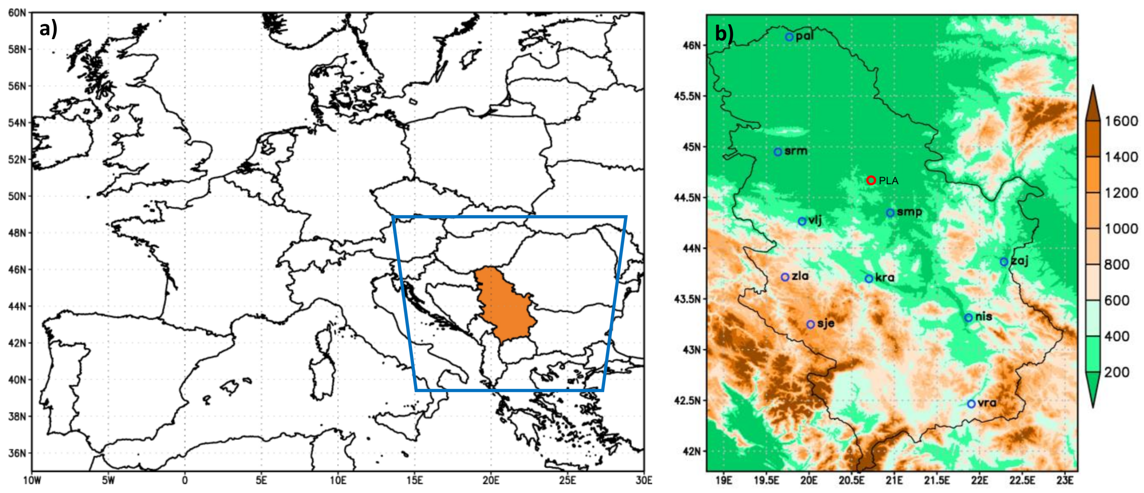
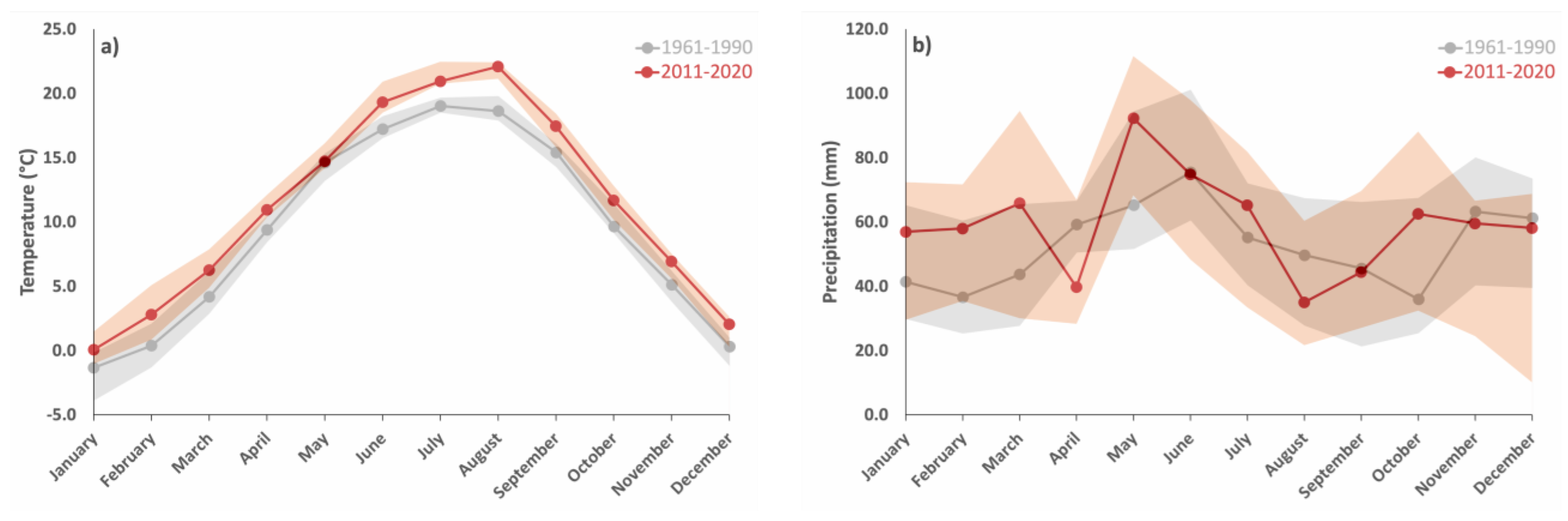
2.1. Description and Capacity of the Study Region

Serbia is in southeast Europe on the Balkan Peninsula and covers approximately 88,500 km2 (Figure 1). It has a population of 6.9 million people. The main terrain features are as follows: the northern area (Vojvodina) is made up of low-land regions and is relatively flat; the central and southern areas are hilly and mountainous, interspersed with low-altitude river basins. The usual climate conditions are a warm temperate continental climate in the lower regions with colder mountain climate features at higher altitudes. Serbia is relatively near to the sea, but the intrusion of maritime climate characteristics is limited by high mountain ranges. The continental climate characteristics include hot summer temperatures and colder winters and in terms of annual precipitation distribution, the highest accumulations occur during the late spring and early summer [2]. Climate change in Serbia has caused significant disturbances in the functioning of different sectors and agriculture has been recognized as one of the most vulnerable sectors, with an urgent need for the adaptation implementation [5,8].
The institution that is responsible for climate services is the Republic Hydrometeorological Service of Serbia (RHMSS). It has a department for agriculture, which provides bulletins on the observed (past) weekly, monthly and annual agrometeorological parameters. The RHMSS is the host of the South East European Virtual Climate Change Center (SEEVCCC), to provide climate monitoring and operational long range forecast (LRF) for the region of South-East Europe (SEE). The RHMSS is also a participant in the SEECOP (South East European Climate Outlook Forum), which provides a consensus (with the participation of other SEECOP parties) on the summer and winter forecasts for the SEE region in textual form, although the information and vocabulary are not fitted for use in decision-making in agricultural production. Improving the climate services of the RHMSS requires an enhanced capacity for technical and human (expert) resources, including upgrading of processing and sharing observed and projected climate data, and building advisory/warning systems, especially those that are user oriented.

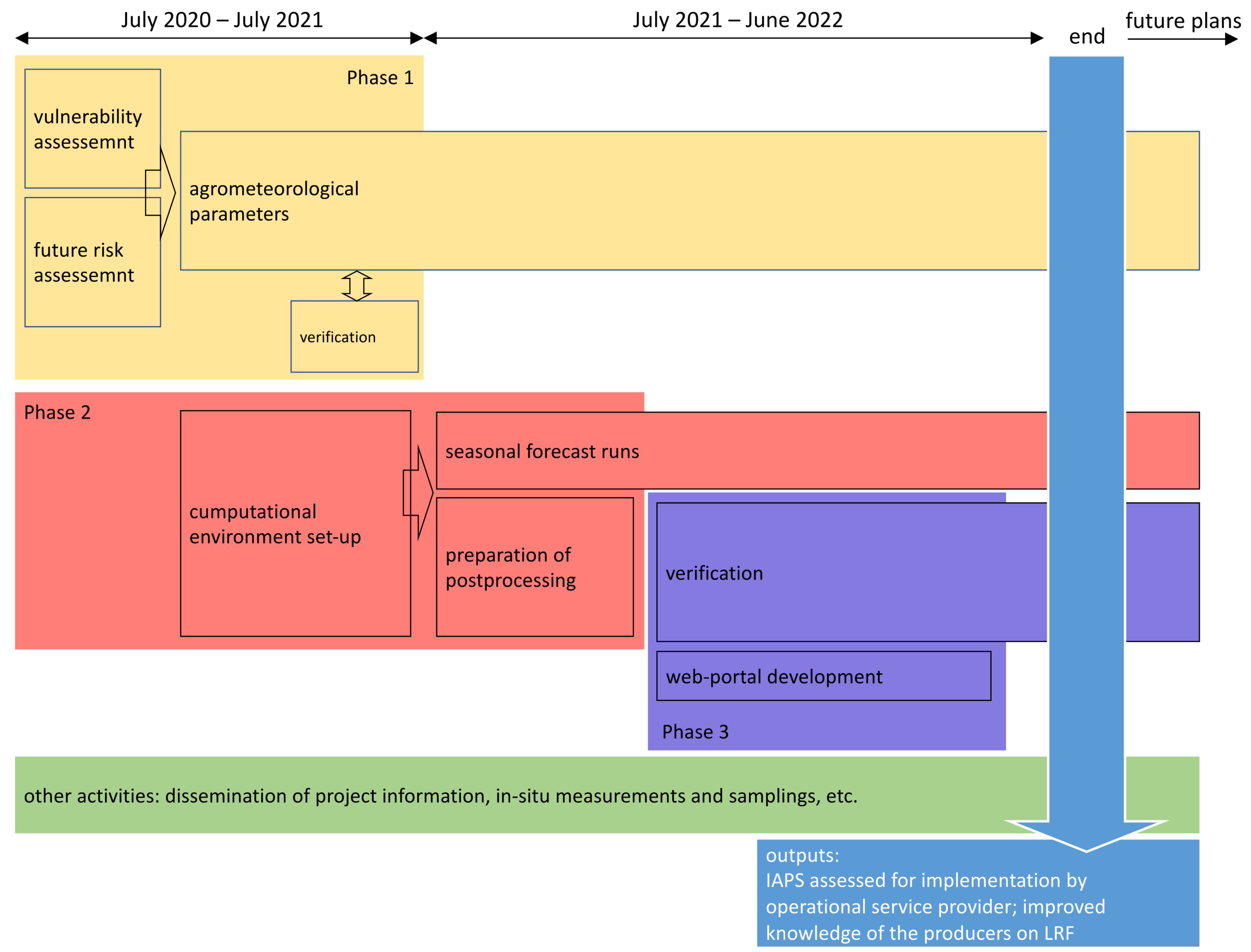
2.2. IAPS Background Information

The Integrated Agrometeorological Prediction System (IAPS) project was granted within national call for early career scientists. A maximum of five early career scientists participated in the project, with one senior scientist who was engaged part time. The duration of the project was 2 years (July 2020–June 2022). During the project, several PhD students were also engaged to help with data collection and learn about the use of long range forecast products and their processing.
The project participants are skilled in weather and climate modeling, climate change impact assessments for different sectors of the economy, agricultural production (fruit, viticulture and wine, crops, etc.) and soil and water management. They had previously been engaged with works that were related to the creation of national documents on climate change and projects that were related to the zoning of agricultural production in the Republic of Serbia, and they had already established connections with agricultural producers. Bearing in mind the project duration and the human and technical resources, project focused on (a) understanding the needs of the users and how to bridge the gap in communication between service providers and service users, (b) assessing whether products could be operational and available for decision-makers and (c) the collection of new in situ data for the selected locations for future studies.
The rapid development of the computational abilities of processors has reached a level that enables ensemble seasonal forecast for the region size such is Serbia to be feasible in a reasonable computational time using desktop computers with the best available processors (i.e., 64-core processors by the time of the project application). This was a major factor that enabled the implementation of the project without previously existing HPC facilities or high levels of IT expertise.
The total budget for the project was EUR 200,000. About half of the total budget was for the salaries of the scientists. The high-performance computing system was about EUR 16,000. The remaining budget was spent on other technical equipment (personal computers, sensors for additional measurements, travel, the dissemination of the project information, etc.).
Figure 2 shows a scheme of the main project activities. Initially, the project activities were designed according to the planned start time of the project, which was at the beginning of the year, but they had to be adapted to the delayed start time, at the middle of the year, because of the COVID-19 pandemic lockdowns. Figure 2 represents the adjusted timetable for the project. The first year of the project was spent assessing the vulnerabilities and risks for agricultural production, based on the most recent climate data (observed and projected). In this phase, climate risk factors were determined, which served as inputs for defining the initial set of seasonal forecast products (agrometeorological parameters). The risk factors were verified with the producers. A questionnaire was conducted among producers to collect information about their practical experience and assess their knowledge and opinions about forecast data (availability and quality). In the meantime, the second phase of the project also began, in which the computational environment was set up for the seasonal forecast operations. In the second year of the project, the seasonal forecast runs began, hindcast tryouts for the test year 2017, and continued with the operational forecast during the project duration. Postprocessing codes were developed to provide forecasts for a defined set of agrometeorological parameters and prepare the outputs for the web portal. In the third phase of the project, the web portal for data dissemination started to be developed (which is currently under construction, along with the verification of the reliability of the forecasts that were performed for the previous period).
Parallel to the above phases, the project also included other activities that served the purposes of disseminating project information to the public, scientific community and producers and providing in situ measurements of the meteorological parameters along with a quality analysis of the products for future work on the development of new agrometeorological parameters that relate weather and yield quality.
There were some setbacks that slowed down the project activities, including the lockdowns in 2020 due to the COVID-19 pandemic and delays in financing and equipment acquisition. For this reason, the second phase of the project started in the first half of 2021 and the seasonal forecast runs were conducted in mid-2021, which was about half a year later than planned. These delays shortened the available time for the preparation and assessment of the seasonal forecast products designed for agriculture and impacted the first year of in situ observations.

2.3. Setup of the Numerical Weather Prediction Model

The regional numerical weather prediction model (NWPM) that was used for this study was a Non-hydrostatic Multiscale Model on a B-grid (NMMB) [26,27]. It was set to run over the domain that was presented in Figure 1 and to provide outputs on every 6 h of the forecast. The initial and boundary conditions were derived from the European Centre for Medium Range Weather Forecasts (ECMWF). It was decided to run the seasonal forecasts for the months of February to September (updated each month) but limit all forecast durations to November, i.e., focus on the conditions that related to the growing season. The seasonal forecast consist of 51 forecasts that form an ensemble and provide a probability assessment of future weather conditions. The forecasts were conducted at a resolution of 0.095° × 0.095° using the best possible computational and time resources that were available. This setup of the forecasting system was assumed to be sufficient for the verification of the quality of the predictions for the identified weather-related risks and for the provision of high-resolution results that correspond to user needs, bearing in mind the relatively small-scale structures of the farms [4].
As the test year, 2017 was chosen as it was the most recent year with high temperature extremes and drought, which were identified as causing the second largest losses in agricultural production after the weather events of 2012 [7]. Hindcasts were carried out for 2017 and afterward, the forecasts continued for the full time period of the project (2020–2022), but only the data from 2017 were analyzed at this point.
The selected postprocessed outputs of the seasonal forecasts were 2-m air temperature, daily accumulated precipitation, soil surface temperature, soil temperature and moisture on 4 depths, 10-m wind, variables that were related to radiation and some other atmospheric variables that were not relevant to this application. Not all of the outputs were required for this study but we chose to store them in case they are needed in future work because the re-runs of seasonal forecasts are computationally expensive. The computational time that was required for the ensemble forecast for 7 months was about 2.5 days, which made it feasible for the computing resources that were available.

2.4. Source of Verification Data

For the climate change analysis, the daily temperature and precipitation data for the period of 1961–2020 were used from the EOBS database [28]. For the verification of the long range forecast products, data from the 10 selected RHMSS meteorological stations (which are distributed across Serbia, as shown in Figure 1) were used. The locations, full names and acronyms of the selected stations are presented in Table 1. The observed dates of the phenophases that were used are from the location of the Plavinci winery. The following phenophases were used for the domestic grapevine variety Panonia: budburst, flowering, veraison and harvest.
The verification of the main risks to agricultural production that are caused by weather extremes was conducted by implementing a questionnaire among producers at the beginning of 2021. More details about this questionnaire are presented in the analysis of our results.

3. Results

The results of the project are discussed in this section, including the climate change vulnerability and risk assessments, the prioritization of the identified risks, the verification of the identified risks by producers and the verification of the LRF results for the test year of 2017. These results led to the initial design of the IAPS and the defining of the gaps and needs for future research.

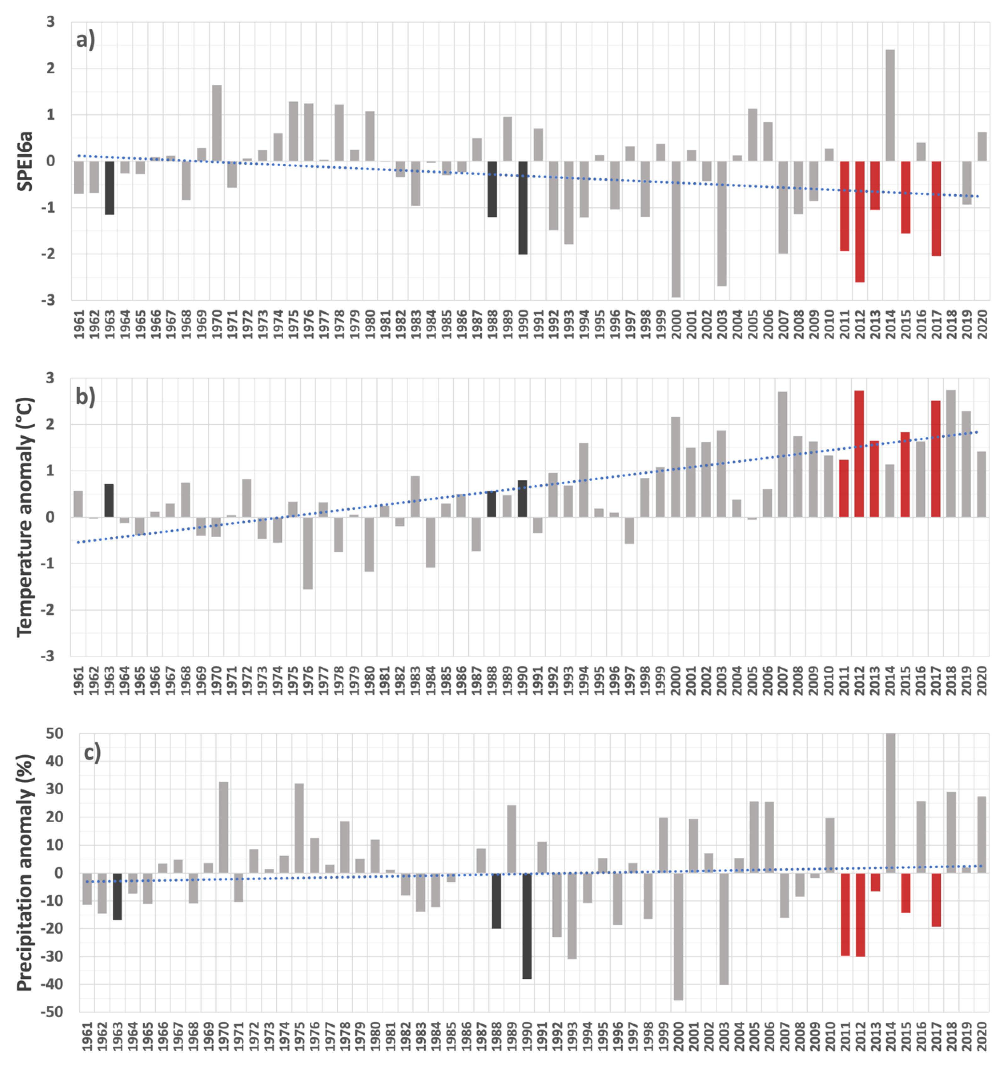
3.1. Selection of Climate Change Risks for Long Range Forecast

Previous climate change analyses on a national level have recognized that climate- and weather-related risks in agricultural production stem from increasing temperatures, heat waves, droughts, the early onset of growing seasons followed by frost, extreme precipitation, hail, strong winds, floods, etc. [4,5]. A more detailed analysis of the vulnerability of fruit production to climate change was conducted during the IAPS project and published in [29]. Increasing temperature conditions have caused climatic category changes in grape growing (the categories are defined by the range of values for specific indices [29]) and a shift in climatic conditions to about 200 m higher in altitude. Climatic categories have changed to more favorable conditions for producing high quality wine and the area that is suitable for grape growing has expanded. This is a single positive example of the impact of climate change in Serbia. The risks that were identified for fruit and wine production are extreme heat during the summer, heat waves in winter and spring that trigger the early onset of growing seasons and increase the risk of frost damage, heavy precipitation and droughts. Most of the areas that have been affected by hot summer temperatures are in the lowlands of Serbia. Areas below 500 m occupy 61% of the territory of Serbia and are mostly cropland. From the more extensive impact analyses for the different subsectors of agriculture, a common problem that is caused by climate change was identified: the disturbance of phenological plant development [30,31].
The rate of temperature change and the problems with droughts have increased during the recent past period. According to the latest results, the average temperature for the period of 2011–2020 (which was the warmest decade in Serbia) was 1.8 °C higher than for the period of 1961–1990. The highest increase in temperature (2.4 °C) occurred in the summer (i.e., June, July and August, JJA). Figure 3 shows the average monthly temperature and accumulated precipitation for both periods (median values and envelope with the range of 25th–75th percentile). The JJA temperature increase could be considered as the most severe since there was no overlapping between the areas of the most probable values (within the interquartile range). This means that the majority of summers in 2011–2020 were warmer or as warm as the hottest summers in 1961–1990. Summer heat waves are recognized as a threat for the agricultural production, causing sunburns on yield, drying of crops, etc. [4]. According to more recent results, it is very likely that previous assessments have underestimated future temperature increases. More likely, the increase in average annual temperature that is expected for 2041–2060 is 3.1 °C compared to 1961–1990 and 3.9 °C for the summer (JJA) average temperature [32]. The monthly precipitation averaged over Serbia do not show any such severe change, and these 10-year averages are highly impacted by the extremes. The precipitation increase in May for the period 2011–2020 is the consequence of the exceptionally high precipitation in May 2014 which caused the severe flood in Serbia. In addition to the increasing temperatures, also happens increasing frequency and severity of the droughts [5].
Figure 4 shows the values of the SPEI6a (the Standardized Precipitation Evapotranspiration Index for a 6 month-period ending with August, which was calibrated for the reference period of 1961–1990) [33], averaged for Serbia, for each year in the period of 1961–2020. The SPEI6a showed a good agreement with the other evidence for the impact of droughts in Serbia. Its variations showed a good agreement with the variations in the total annual corn yield, which is very vulnerable to droughts [7]. SPEI6a values that are less than −1 represent years with drought in Serbia. The results show that during the period 1961–1990 only 3 years were with drought (dark grey), according to this criterion, and during the decade 2011–2020 5 years were with drought (red). More frequent and more severe droughts have occurred since 2000. To better understand the main cause of these increasing droughts, the anomalies for the average temperature and accumulated precipitation for the period of March–August are also shown in Figure 4, compared to the average values for the period of 1961–1990. The increasing trend of temperature change is evident, while the trend of the precipitation change shows small increasing, which was not significant.
During the late 20th century and the beginning of the 21st century, Serbia was affected by a lack of precipitation, which caused drier conditions. Afterward, the average annual accumulated precipitation increased, but the temperature increase continued at a higher rate and caused drier average conditions besides the fact that average total precipitation also have increased [32]. This means that under warmer conditions the same amount of precipitation as in the reference period was insufficient to maintain the same humidity of the climate. Additionally, as shown in Figure 4 and discussed in [2], the variability of precipitation increased (i.e., the accumulated precipitation deviate more from the average climate values) compared to that during the reference period. This produced higher frequency of the years with larger precipitation deficit, which combined with the temperature increase as an amplifier caused more years with drought.
Comparing values of temperatures and precipitation for the years with drought during the recent period, for example 2011–2020, with drought years in the 20th century, it can be concluded that increased temperature has significant contribution to the drought events.
Bearing in mind all of the impacts of climate change, a questionnaire was conducted among producers to identify the most important risks to address by using long range forecast products. Replies were received from 268 agricultural producers. The amount of agricultural land that was worked by the respondents was about 1% of the total agricultural (arable) land in Serbia (about 70% of the Serbian territory is agricultural land) and their farms were in all 24 counties in Serbia (without Kosovo).
The most relevant information, which was derived from the questionnaire, is presented in Figure 5. More details about the questionnaire are included in Appendix A. Over 50% of the respondents had farms (total property) of 1–10 ha, almost 30% of the respondents had farms of 10–100 ha and six respondents had farms of over 1000 ha. Almost 50% of the producers had farms that were below 200 m of altitude and almost 40% of the farms were in the range of 200–500 m of altitude. Only 13 respondents had farms that were over 800 m of altitude. The questionnaire was conducted to collect feedback from the producers regarding which weather hazards impacted their production the most. They were asked to assess the levels of damage that weather hazards had caused to their production.
The highest average grades were for high summer temperatures, frost in growing season, high wind, hail and drought. Low winter temperatures, showers (extreme rainfall), floods and others had much lesser impacts (as shown in Appendix A). The causes of high levels of vulnerability for production below 200 m (not shown in this paper) were indicated as follows: 28% of the respondents identified drought, 23% identified high summer temperatures, 22% identified hail and frost in growing season and high wind were identified by 15% of the respondents each. In total, the medium and the high vulnerability of production below 200 m, 69% of the respondents identisied for the high summer temperatures, 69% for the drought, 66% for hail, 63% for frost in growing season and 52% for high wind. Accounting all the respondents’ assessments (with farms in all altitudes, Figure 5), high level of vulnerability for drought is identifies by 27% of the respondents, for high summer temperatures by 18%, for hail by 26%, for frost in growing season by 16% and for high wind by 13%. In total, the medium and the high vulnerability of production of all respondents, 68% of the respondents identified for high summer temperatures, 73% for drought, 69% for hail, 62% for frost in growing season and 51% for high wind.
Since hail and wind gusts are local and short-term events, they are possible to predict using high-resolution short-term forecasts and nowcasting; therefore, they were not topics of interest in this project. Meteo-alarm, which is the service that is provided by the RHMSS, regularly issues warnings about these events. Development of the prediction of frost in growing season is highly dependable on the crop variety because of the different heat demands for the onset of growing season, and the required knowledge on plant phenology. Predictions for risk from frost in growing season were not analyzed in this study.
The producers confirmed that the prediction of the priority risks well in advance would enable them to implement on-time measures for short term adaptation (adjustments) of the production. The rest of the information that was derived from the questionnaire is shown in Appendix A.
From previous studies and the presented analysis, we decided to focus the LRF evaluation on summer heat conditions and droughts during 2017. A case study was also conducted at one location to evaluate the prediction of the dates of the phenophases.

3.2. Long Range Forecast Results and Evaluation

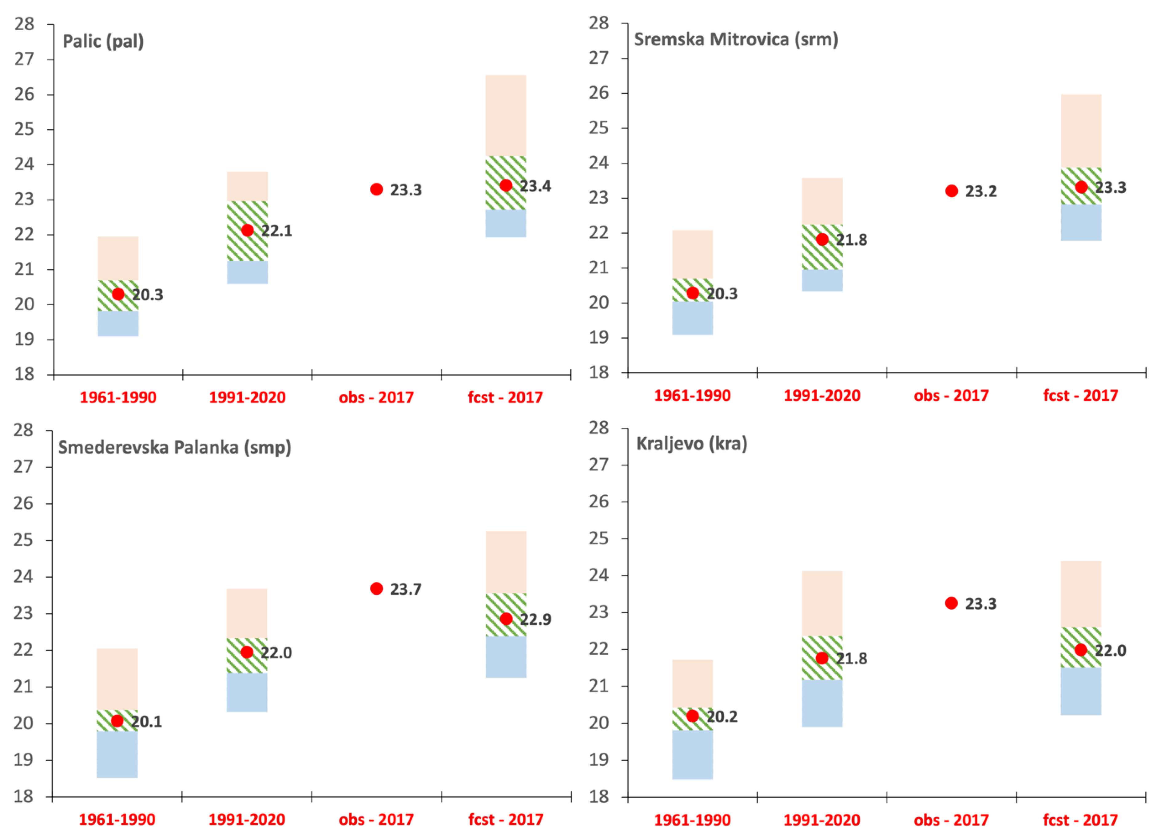
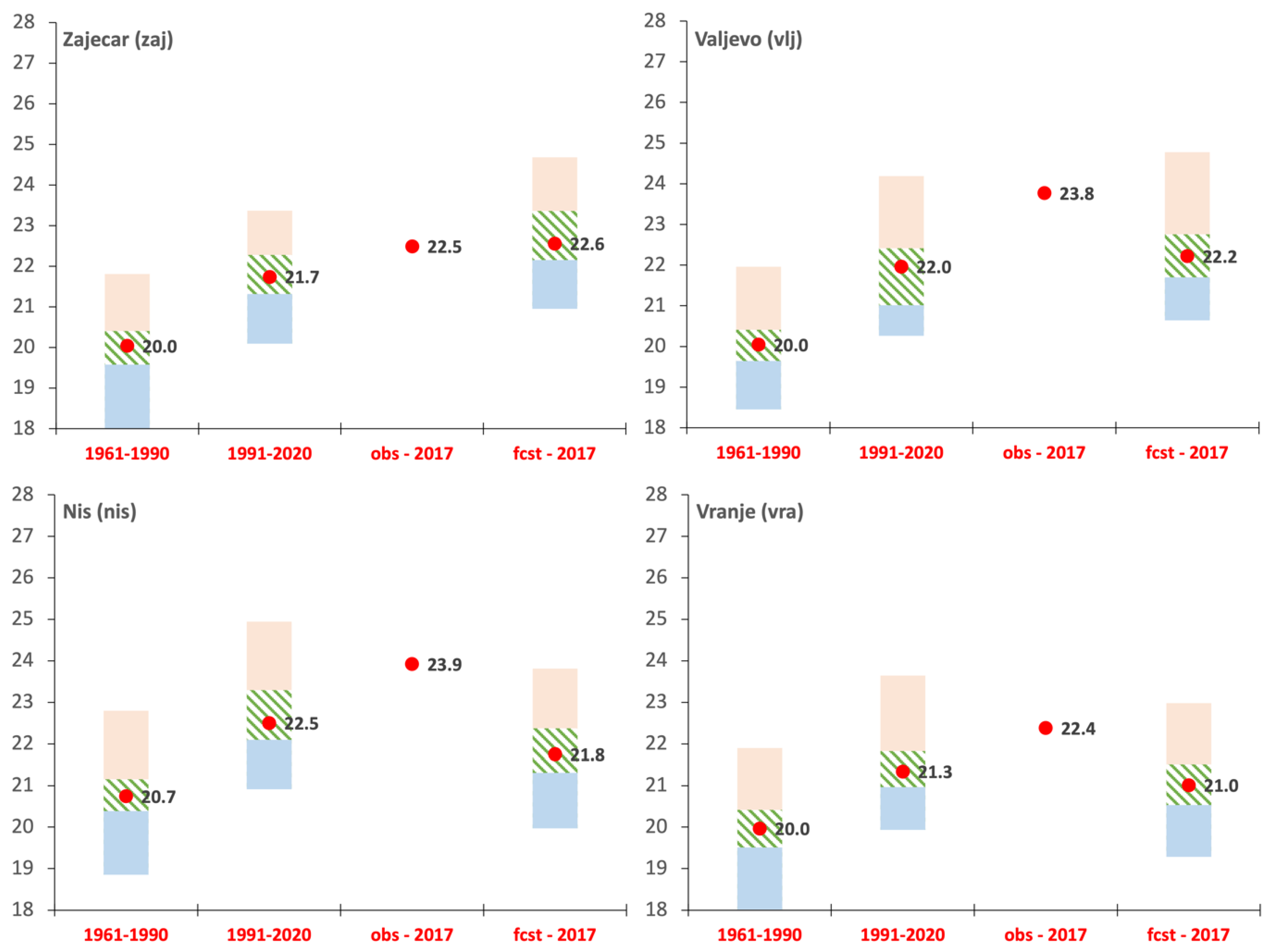
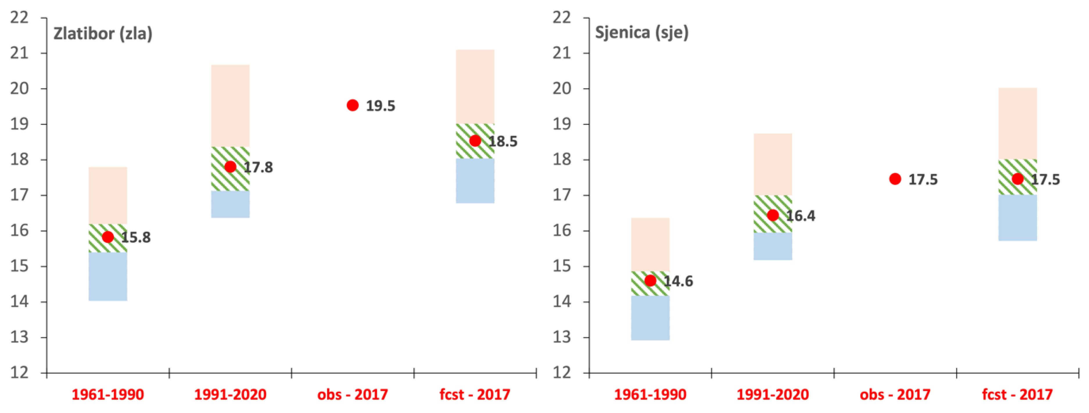
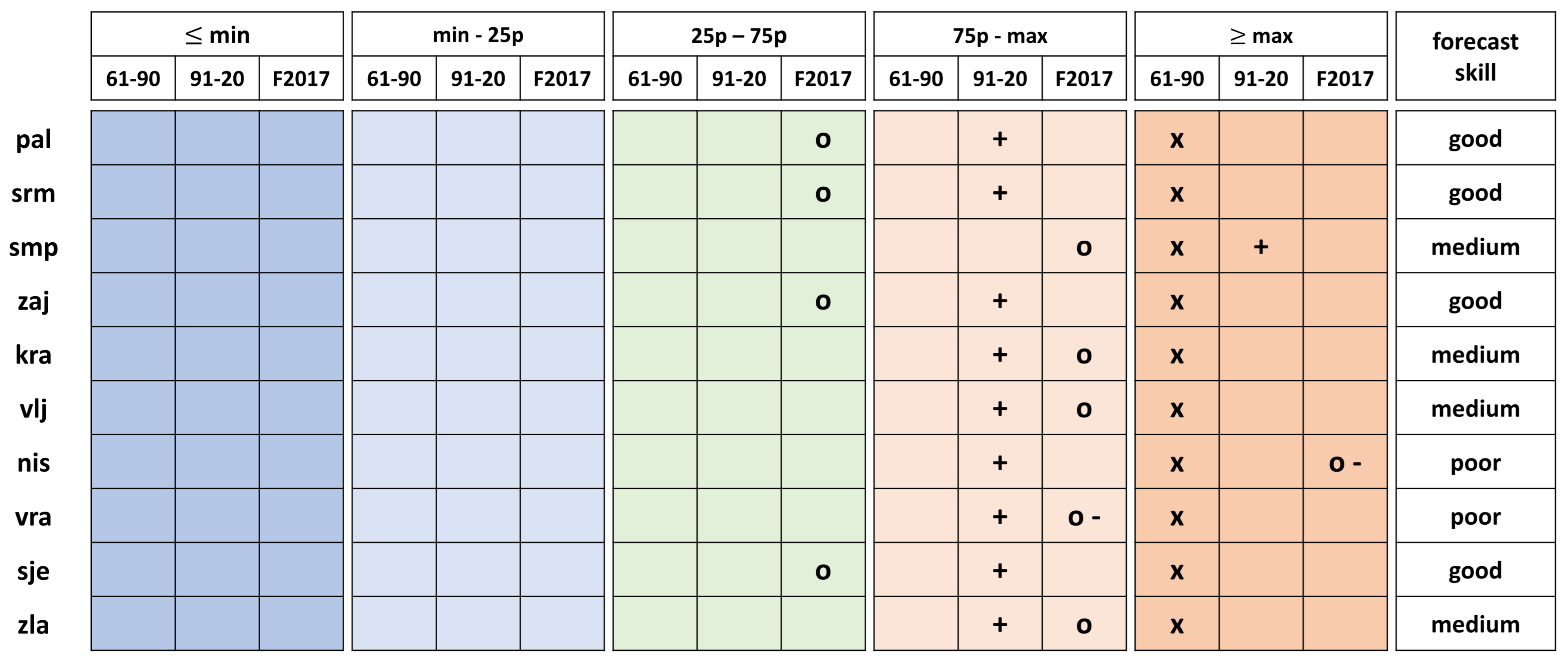
3.2.1. Forecast of Average Summer Temperature

For the summer (JJA) of 2017, the LRFs from February and March (not presented in this study) did not predict such extreme warm conditions, as did the forecast initiated on 1 April 2017. The results of the ensemble LRF forecast were compared to the observations from the 10 selected stations (Figure 1 and Table 1). The reason that we decided to compare the forecasts to in situ meteorological observations rather than for the whole Serbia using, for example, EOBS database, was that we did not want to add another uncertainty into the assessment. In this way, the results were compared to values that were observed and were the most accurate. All of the selected stations conducted continuous measurements for the whole period that was needed for this assessment, i.e., 1961–2020. The summer of 2017 was ranked as one of the six warmest summers on record at the selected locations during the period of 1961–2020 (first place at one location and second place at four locations).
Only information publicly available from the climate service (easily accessible) for the producers are average climate values for the period 1991–2020. This climate period was considered to be representative of the current conditions, besides the fact that each decade within this period was notably warmer than the previous. We wanted to assess whether LRF could provide better information about summer temperatures than climatology. This meant assessing whether the LRF results were closer to the observed average summer temperature than the average climate value and whether they showed a good sign of anomaly (above/lower than average climate value). If this is fulfilled, we consider that the forecast provided useful information. To better understand the severity of forecasted event, the analysis also included observed values from the reference period 1961–1990.
For each climate period (1961–1990 and 1991–2020), for the average summer temperatures, besides average values, are calculated minimum, 25th and 75th percentile, and maximum values. The same values were calculated from the ensemble seasonal forecasts. Figure 6 shows in which range of values belongs observed average summer temperature, for the two climate periods and for the ensemble forecast. The results that were obtained for each station separately are provided in Appendix B.
The forecast skill that is shown in Figure 6 is defined according to following:
  • “Good”: when the observed value is within the interquartile range (25th–75th percentile) of the ensemble forecast and the forecasted (ensemble median) anomaly (warmer/colder) compared to the average climate value has the same sign as the observed anomaly;
  • “Medium”: when the observed value is closer to the forecasted (ensemble median) value than to the climate value; the observed value is outside of the most probable range of the ensemble forecast results (25th–75th percentile) but within the ensemble total range of values (min-max); the forecasted (ensemble median) anomaly (warmer/colder) compared to the average climate value has the same sign as the observed anomaly;
  • “Poor”: when the forecasted (ensemble median) anomaly has the opposite anomaly sign compared to the average climate value to the observed anomaly and/or the forecasted value is outside of the ensemble values.
Considering the above, when the forecast skill is ranked as “good” it provides reliable information to the users than the climatology, and when it is ranked as “medium” it provides more useful information than climatology
The summer of 2017 was warmer than warmest summer during the period 1961–1990 (marked with an “x” in Figure 6) at all stations, which shows that the temperature conditions were exceptionally warm with the respect to the summer conditions in the 20th century.
Average JJA temperature for the year 2017 compared to the 1991–2020 was significantly warmer than average. At nine stations, it was between the 75th percentile and the maximum value (marked with a “+” in Figure 6) and it equals the maximum value at one station. At eight stations, the median of the forecast was closer to the observed value than the climate average and indicated warmer than average conditions (“medium” and “good” forecast skill), out of which in four stations the forecast skill was “good”. In two stations the forecast skill was “poor”, since it showed colder than average values and in one the full ensemble range (max-min) was lower than the observed value.
Lesson learned from this case study is that the forecast skill is best in the flat terrain in north Serbia (pal, srm), in east Serbia (zaj) and in flatter high altitudes in west Serbia (sje). In other areas forecast bias is higher, especially in south and southern part of Serbia (nis, vra). There are many possible reasons that may cause the forecast bias. For example, the environmental conditions in which the measurements are performed may differ from the input information available to the model. Considering that the long range forecast did not use model climatology to reduce the model bias and, besides that, in the majority of investigated locations forecast skill was satisfactory, the conclusion is that such agrometeorological seasonal prediction system can be of use to the producers in some regions of Serbia. Further work should be implemented to evaluate the model performance for other years, and to learn more about the model bias.

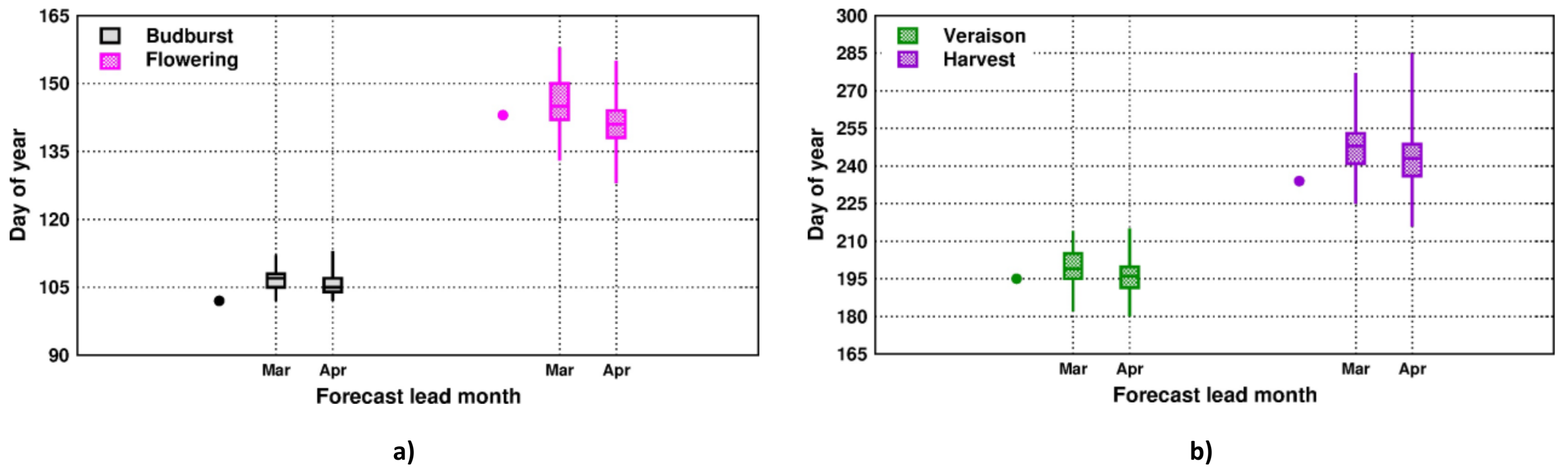
3.2.2. Forecast of Phenological Development

To assess the capacity of the LRF to predict certain events that are relevant for agriculture, a case study was conducted for the grapevine growing season phenology at the Plavinci winery (the location of which is shown in Figure 1 and Table 1) for 2017. Only this location provided enough data to implement this calculation. The case study was conducted on the domestic grapevine variety Panonia. The producer installed a meteorological station and provided the phenology data for the period of 2015–2021. Using the observed temperature data and the observed dates for budburst, flowering, veraison and harvest, the criteria were determined for the average growing degree days for each phenophase.
Figure 7 shows the observed dates of the phenophases and the forecasted dates from the ensemble LRF forecast, which were obtained from the forecasts that were initiated in March (leading month 3, LM03) and April (leading month 4, LM04) 2017. The median values of the ensemble forecast were considered to be representative. The results showed the following differences between the forecasted and observed dates:
  • Budburst: 5 days in the March forecast and 3 days in the April forecast;
  • Flowering: 2 days in the March forecast and −2 days in the April forecast;
  • Veraison: 4 days in the March forecast and 1 day in the April forecast;
  • Harvest: 14 days in the March forecast and 9 days in the April forecast.
Figure 7. The observed (dots) and forecasted dates (ensemble spread: minimum, 25th percentile, median, 75th percentile and maximum) for budburst and flowering (a) and veraison and harvest (b) at the Plavinci winery in 2017; the forecasts were initiated in March (Mar) and April (Apr) 2017.
Atmosphere 13 01337 g007
The April forecast gave somewhat improved prediction compared to the March forecast. Forecasted dates show difference compared to the observed dates in the range 1–3 days for budburst, flowering and veraison. Both forecasts predicted later harvest dates than were observed. The producer did not wait for physiological ripening to occur and instead harvested the yield when there were enough sugars for the production of wine. This was the reason that the predicted harvest dates and the observed harvest dates differed more than the dates for the other phenophases.
This case study showed the great potential of the use of forecasted growing degree days in the prediction of phenophases well before their occurrence. Other results, related to this case study, are presented in Appendix C.

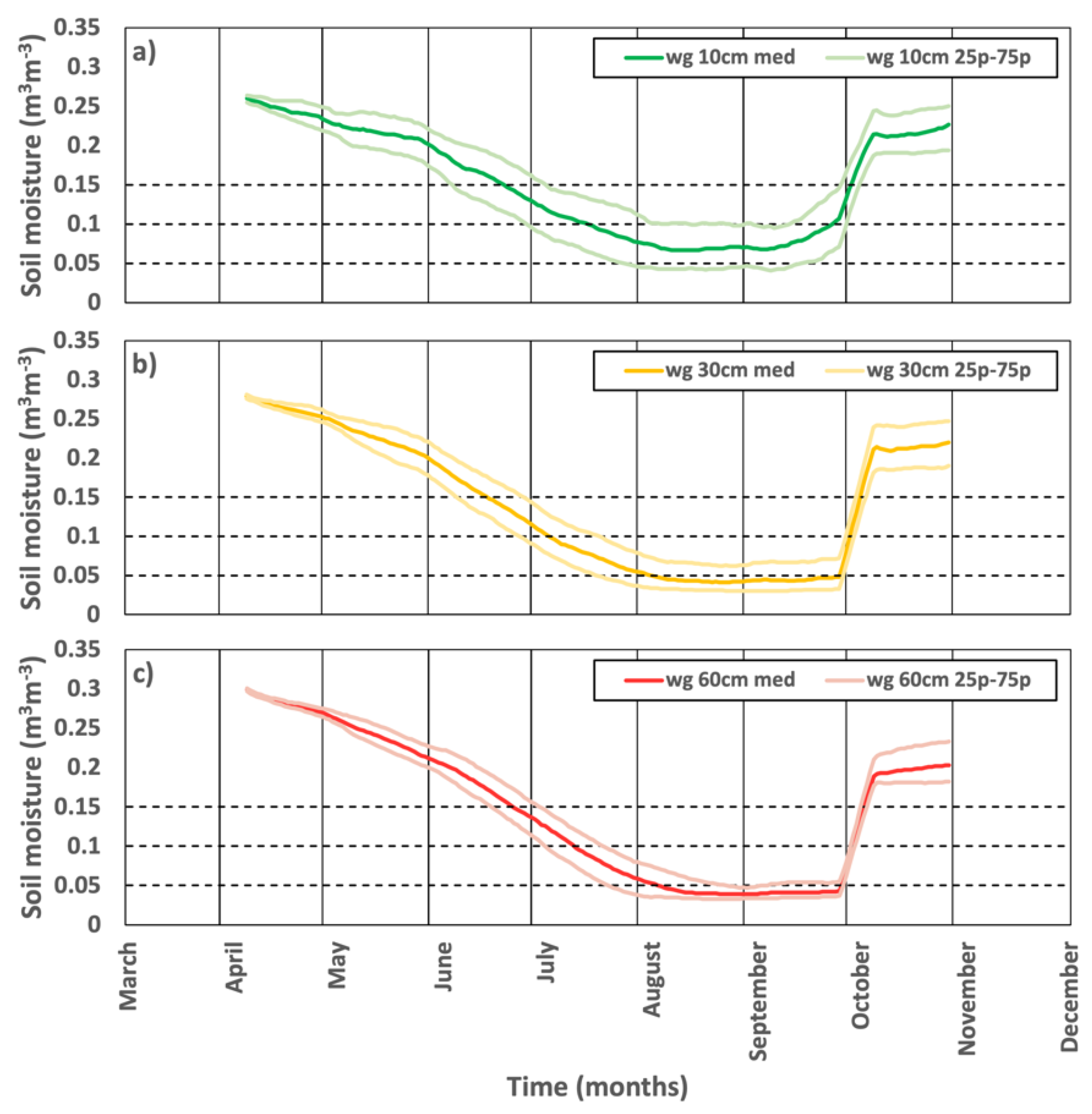
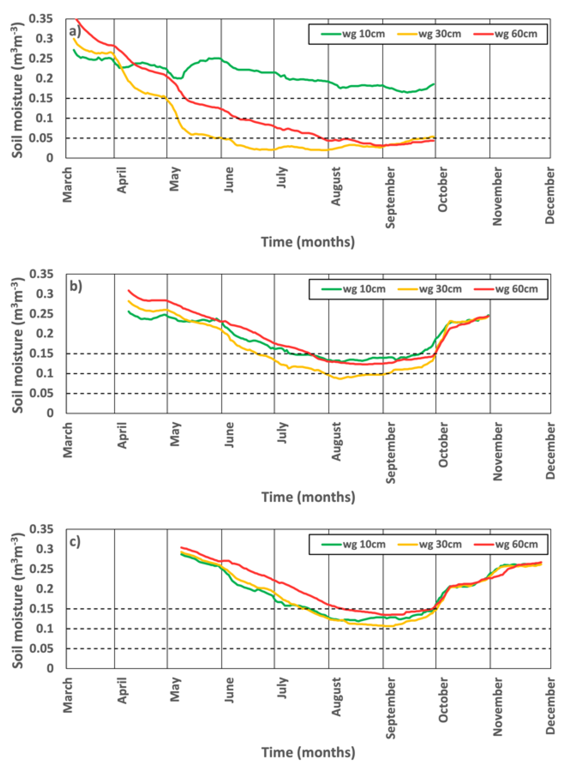
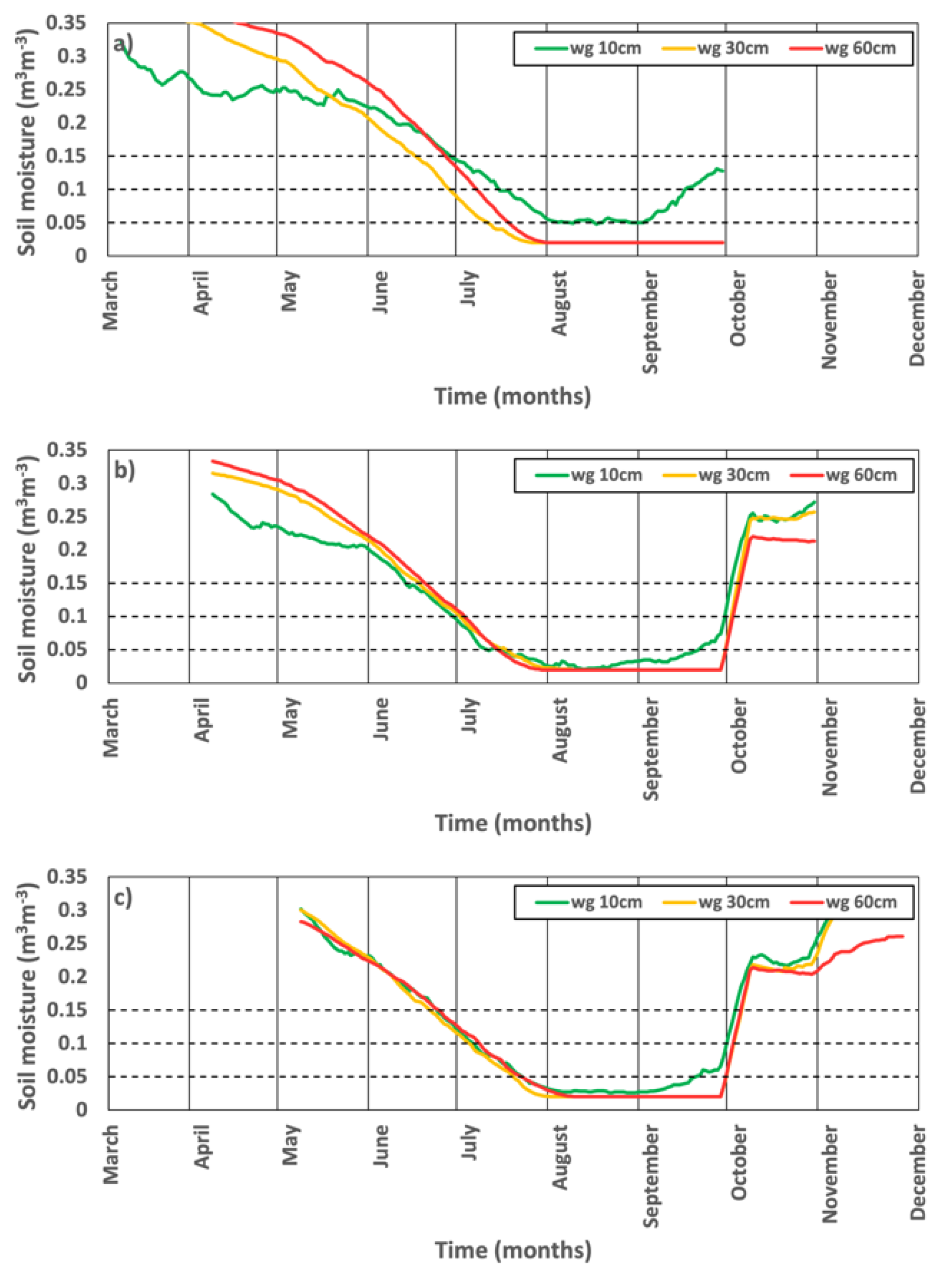
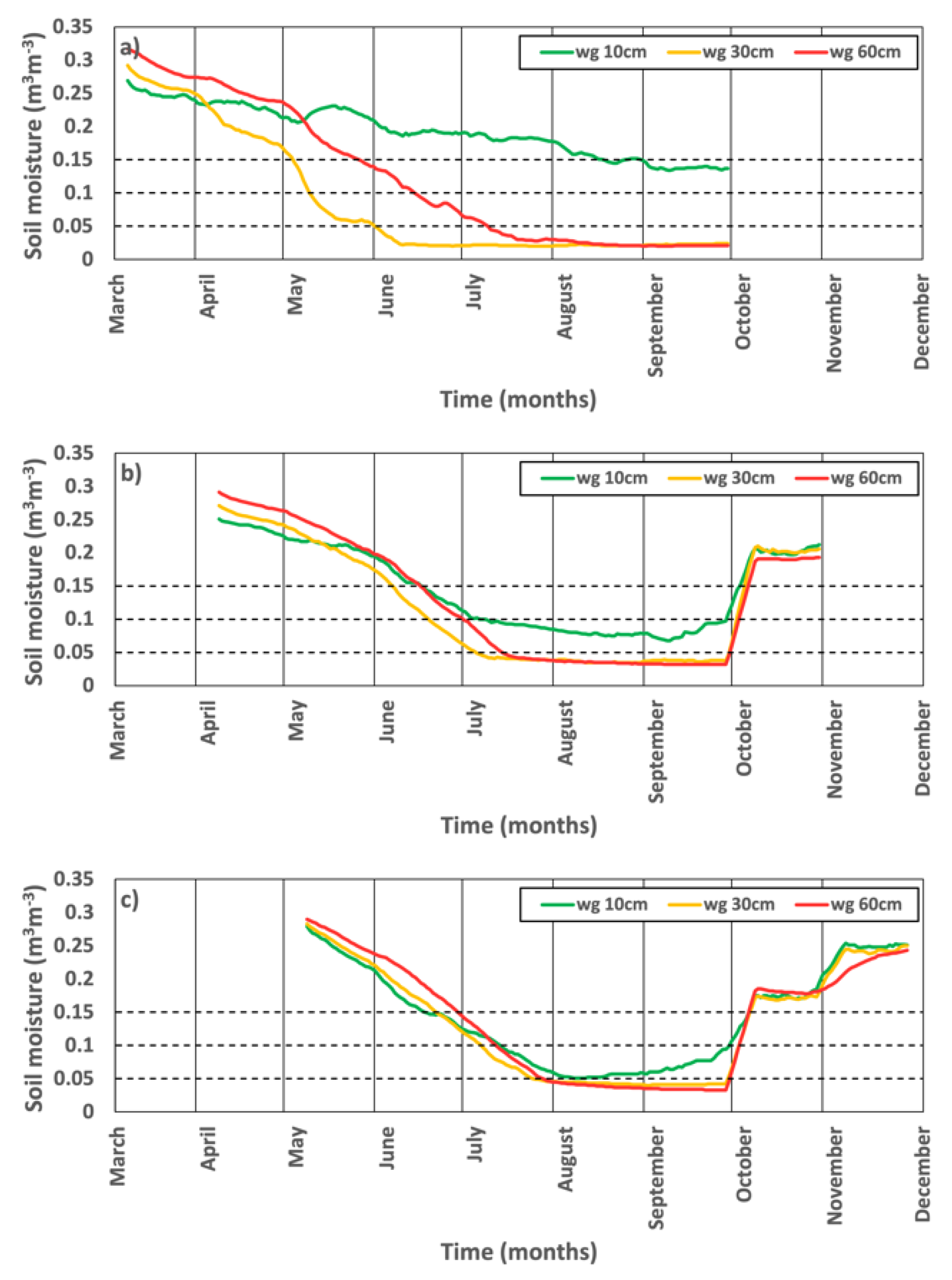
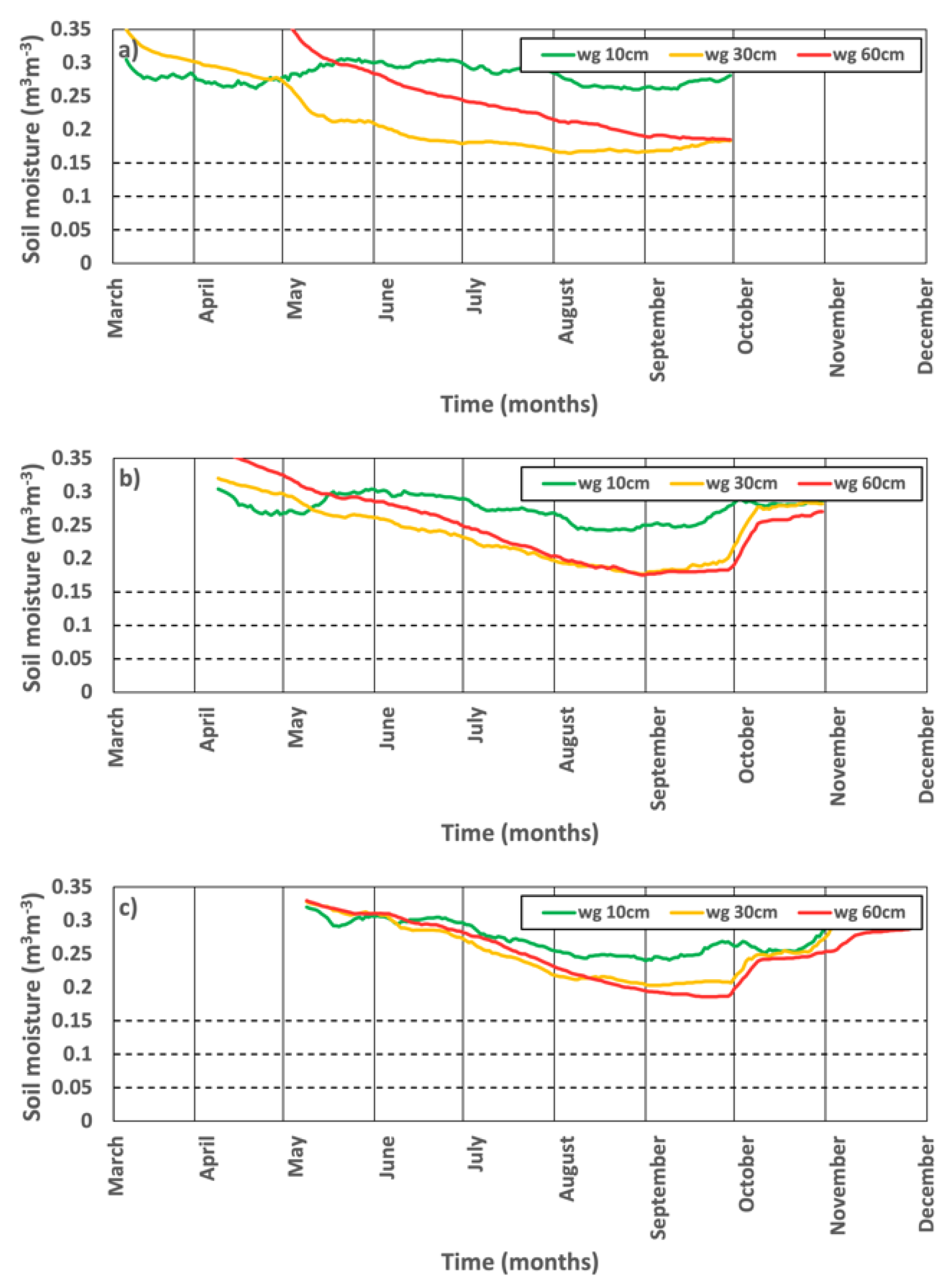
3.2.3. Drought Forecast

In agriculture, drought means that there is not enough water available in the soil for the development of plants Soil moisture on different depths in the models are the prognostic variables and depend on the heat- and water-related conditions, characteristics of the land cover and soil properties. While the seasonal precipitation prediction has large uncertainties, for the prediction of the soil moisture is considered to have the ability to transform less predictable precipitation signal, including the impact of heat conditions and other land surface processes, into more predictable soil moisture signal [34]. Also, the soil moisture, especially in deeper levels, beara a memory of the moisture conditions during the longer period. It is not very sensitive to short term high precipitation which do not infiltrate the soil as much but can cause the false conclusion for the analyzed period (month, growing season) that there was sufficient water available for the plants development. LRF forecast uncertainty is much larger for precipitation than for temperature (not shown in this paper), so it is best to avoid their use, when possible, for assessing agricultural drought conditions. Another significant factor for droughts is high temperature conditions that evaporate the available water faster. During growing seasons, root extraction of water is another significant factor In the model, soil moisture prediction includes the physics of the processes which impact water availability in the soil. Therefore, it is expected that the predicted soil moisture will provide much more reliable information on drought than drought indices.
LRF results were obtained for soil moisture contents at the following depths: 10 cm (representative for the layer of 0–20 cm), 30 cm (representative for the layer of 20–40 cm) and 60 cm (representative for the layer of 40–80 cm). The latter two depths (deeper soil) were more important for assessing agricultural droughts because the root systems of the cultivated varieties are on those depths. An analysis was carried out for the forecasts from March, April and May 2017 for the same locations as the summer temperature analysis (Figure 1 and Table 1). There were no measurements of soil moisture, so the verification of the LRF skill only relied on the following criterion: when the LRFs for soil moisture produced dry soil conditions (no available water for plant development), the forecast skill is good. Dry soil was expected to be forecasted at the majority of the selected locations.
The results for all locations and additional comments on this case study are provided in Appendix D. The forecast that was initiated on 1 March 2017 predicted that dry soil conditions will happen during the summer, in the second part of July and will last during the August and September. The same signal was observed in the forecasts from April and May. In eight out of the ten locations, soil moisture values were below 0.05 m3m−3 (equal or close to the so-called “wilting point”). The forecasts that were initiated later predicted that the onset of dry soil conditions will occur later, which was related to the initial conditions of the soil moisture and the time that was needed for the soil physics in the model to reduce the soil moisture at deeper layers (the results are shown in Appendix D). The quality of the initial soil moisture values is affected by the lack of soil moisture observations from Serbia.
As an example, the results from the forecast that was initiated on 1 April 2017 are presented in Figure 8. They represent moving 10-day averages (the values were assigned on the fifth day of the 10-day period) for the locations at lower altitudes (eight locations) because agricultural production mostly occurs at lower altitudes. Three threshold values are marked with a dashed line, which represent the threshold values for dry soil conditions for different soil types (as explained in Appendix D). Soil moisture content in the range 0.1–0.15 m3m−3 means that the soil is “dry” for the soils with more clay content. Soil moisture content lesser than 0.05 means dry soil for the soils with more sandy content. The results showed that there is a 75% probability that the soil will be close to dry or completely dry (without any available water) at lower altitudes and most probably (median values) will reach exceptional drought in deeper levels in August and September. As mentioned before, the threshold values varied depending on the soil properties. For some soils, the wilting point is larger than the 0.05 threshold. So, in the future development of this forecast system, the threshold values should be revised and adjusted for specific locations (a related discussion is presented in Appendix D).

4. Discussion

The Integrated Agrometeorological Prediction System (IAPS) project was designed according to identified needs to enhance the national capacity for improved climate services for agricultural production. Its main goal was to create a forecasting system that could provide real-time information for decision-making among agricultural producers regarding the implementation of the actions that could reduce the losses and costs that are caused by increasingly unfavorable (extreme) weather conditions. While most agricultural production involves annual crops, fruit production and viticulture are much more affected by climate change because of the constant exposure to weather conditions and the transferable damages to the next year.
According to our analysis of the climate change impacts on agriculture and the feedback from producers, the main risk factors for agricultural production that could be predicted with LRF are high summer temperatures and drought. According to previous studies and observed climate change impacts, the disturbance of phenological plant development is also of great interest for producers. When this project started, 2017 was the most recent year that had extremely warm summer temperatures and droughts and resulted in a great loss of agricultural production, so it was chosen for the initial evaluation of LRF capacities in terms of producing useful information for producers.
Long range forecasts were produced using the regional NMMB model at about a 10 km resolution for a period that includes the growing season of plants that are cultivated in Serbia (approximately April–October). The initial and boundary conditions were used from ECMWF IFS and they consist of 51 ensemble members. Ensemble forecasts provide the probability of the future weather conditions, which is an added value for the decision-makers.
The results show that the forecast can produce the quality results for the variables which bear the memory of the longer period. Those variables are the soil moisture content and related prediction of the agricultural drought, and growing degree days for the dates of the phenophases’ occurrences. The prediction of the summer temperature had a good skill over some, mostly flatter, terrains and provided usable information for producers at the majority of the analyzed locations. In southern parts of Serbia, the forecast significantly underestimated the observed values. Spatial variability of the forecast quality means that model bias should be more investigated. So far, model climatology has not been developed for LRF because of the limited timescale of the project.
Other findings that were not discussed in this manuscript included the following: the prediction of seasonal precipitation had large uncertainty (large range of the ensemble forecast results) and the model could not provide quality information about the number of days with high temperatures. The model outputs were the temperature every six hours. We used the lowest value out of the four daily values as the daily minimum and the highest as the daily maximum and found that the model severely overestimated the number of days with tropical nights and underestimated the number of days with maximum temperatures above 35 °C. For this reason, the daily maximum and the daily minimum temperatures needed to be included as the model outputs because the daily extremes could be reached within the 6-h window (in the summer in Serbia, the minimum temperature is reached between 2 a.m. and 8 a.m. and the maximum temperature is reached between 2 p.m. and 6 p.m.).
According to our results, this LRF system can be used in the operational forecast for agricultural drought using soil moisture content and for the prediction of the phenological development in case data on phenological development are available. These capacities of the LRF system were also proven in [20,34]. For the prediction of summer heat conditions, the LRF system needs to be further tested by developing hindcast for longer period (for example 5 or 10 years) to evaluate the model bias and its consistency among the forecasts for other years.
To provide more LRF products for agricultural producers, the project participants, in collaboration with the PhD students, started field observations at 10 locations for grape growing, 19 locations for different fruit trees and 2 locations for annual crops. Those data will be used for the future development of new LRF products for different varieties and for the verification of the LRF performance.
During this project, information about the IAPS was disseminated through public media on multiple occasions. The Faculty of Agriculture at the University of Belgrade hosted a conference that was funded by the IAPS project and was open to all stakeholders. That was the first conference in Serbia that was fully devoted to climate change and agriculture and it was the first time that the results and capacities of IAPS were presented [35]. The producers expressed great interest in the IAPS products, even with its current limitations, and stated that this information would help them to plan their production, implement timely agrotechnical measures to reduce losses, implement optimal and timely irrigation and plan the employment of field workers, among other actions.
One of the largest obstacles to disseminating LRF information, even when they are conducted operationally, is how a producer accesses the information for the location of their individual farm. The development of a web portal that could provide this access was one of the tasks of this project, which was exceptionally limited by the allocated funds. The project reviewers required the cost of this component to be reduced to EUR 4000 from the initially planned EUR 10,000. To support the dissemination of seasonal forecasts to users with georeferenced geographical coverage, the web portal needs to be interactive, to be supported by a database of georeferenced data and to have a dynamical structure (in which it receives new forecasts and keeps old forecasts). Software developers who could create such a database and web portal are far beyond the funds for this project (approximately by one order of magnitude).
One of the major obstacles to the dissemination of weather- and climate change-related information to the public in Serbia is the poor levels of investment in IT support and software (web) development, which is similar for the technical support in scientific institutions. If this problem is not addressed, the dissemination of useful information and data to producers, scientists from different fields of expertise and other stakeholders will be inhibited and the system cannot be implemented for better future preparedness, and risk and costs reductions. The fact is that in only two years that had droughts (2012 and 2017), Serbia lost USD 3.5 billion in grain production because of the droughts [7] and investments in LRF development and dissemination are about 0.01% of that amount, when the costs of this project and additional costs for information dissemination are considered. The estimated total costs for enhancing the capacity of agrometeorological services (including measurements, forecasts and education) in Serbia (specifically in the RHMSS, as the responsible institution) are about EUR 11.6 million [8], i.e., 0.3% of the loss in agricultural production that was experienced during two extreme years.
Measures for the improvement of agrometeorological services are planned to be included in the National Adaptation Program and its first 3-year action plan (which is under construction), according to expert assessment and recommendations [8]. If adopted as expected by March 2023 (according to the Law on Climate Change), this could be an excellent basis for applications for the funding from the global and inferential funds that are dedicated to adaptation to climate change.

5. Conclusions

Seasonal agrometeorological predictions can provide real-time useful and quality information for agricultural producers, which can enable them to plan and implement actions for short-term adaptation to climate change (so called “adjustments”) of their production. These actions would mitigate the negative impacts of extreme weather conditions that are caused by climate change and enable producers to seize any potential opportunities.
In agricultural production in Serbia, priority climate change risks with increasing impact trends have been identified, which can be predicted using long range forecasts well in advance. These risks include agricultural drought, high summer temperatures and the disturbance of phenological development (including the risk of late spring frosts). Long range forecast of the variables which have the memory of the longer period have the best forecast performance. For this reason, for the drought is advised to use soil moisture prediction and for the phenological development prediction the growing degree days from the start date of the growing season. The forecasts can provide useful information for summer temperature conditions in some areas but require more study regarding bias identification and reduction. Considering the urgency of the problem of climate change impacts on agricultural production, the implementation of agrometeorological LRF prediction system is urgent and necessary to reduce losses. According to the feedback from producers, the current capacity of LRF results are of use to them to implement certain measures for the protection of their production.
Because the costs of the required technical equipment are affordable and the expertise that is required for forecast implementation exists in the RHMSS, the execution of operational forecasts should be achievable in short period; however, the dissemination of the forecast data to the agricultural advisory services and producers is another essential task that requires proper investment for the development of the web portal (and other tools for dissemination), promotions for raising awareness about the existence of the information and the education of stakeholders. The total costs that have been assessed for the improvement of agrometeorological climate services, including seamless forecasts and the dissemination of information, are approximately three orders of magnitude lower than the costs of the losses in agricultural production that were observed just in two extreme years.
Parallel to the operational dissemination of long range forecast data to users, further development of the system is necessary and require engaging the scientific community. The forecast system should be further tested to learn about the forecast bias when predicting different agrometeorological parameters and increase the forecast performance. Collecting and integrating more agricultural and meteorological data could serve the purpose of developing other forecast output data, such as other weather-related risks for different subsectors of agriculture, the probability of yield quality and quantity under upcoming weather conditions, etc.
This LRF system could be used for short-term adaptations in agriculture and could also provide benefits for other sectors that are impacted by climate change, such as forestry, water management, healthcare, energy production, etc.

Author Contributions

Conceptualization, A.V.V., M.V.M. and B.C.; methodology, A.V.V. and M.V.M.; software, V.D.; validation, A.V.V., M.Ć. and A.L.; analysis, A.V.V., M.V.M., M.Ć., D.S. and D.V.; resources, M.V.M.; data curation, B.C., Z.R.-V., D.N., D.S. and D.V.; writing—original draft preparation, A.V.V. and M.V.M.; writing—review and editing, M.Ć., Z.R.-V. and D.N.; visualization, A.V.V., M.V.M. and A.L.; supervision, Z.R.-V. and D.N.; project administration, M.V.M. All authors have read and agreed to the published version of the manuscript.

Funding

This research was funded by the Science Fund of the Republic of Serbia through the PROMIS “Integrated Agrometeorological Prediction System” (IAPS) project under grant number 6062629.

Institutional Review Board Statement

Not applicable.

Informed Consent Statement

Not applicable.

Data Availability Statement

Not applicable.

Conflicts of Interest

The authors declare no conflict of interest.

Appendix A. Supplement to the Analysis of the Questionnaire for Producers

In this appendix, we present additional information about the questionnaire that was conducted by the IAPS project in order to collect knowledge from producers regarding their awareness of the severity of weather hazards, their activities and opinions related to the monitoring and forecasting of meteorological parameters, their awareness of the potential benefits that they could receive from long range forecasts (LRFs), and their trust in the forecast data and willingness to use this information in decision-making to reduce the risk of damage from extreme weather events.
The questionnaire comprised 22 questions, which provided the following information:
  • County of residence;
  • Municipality of residence;
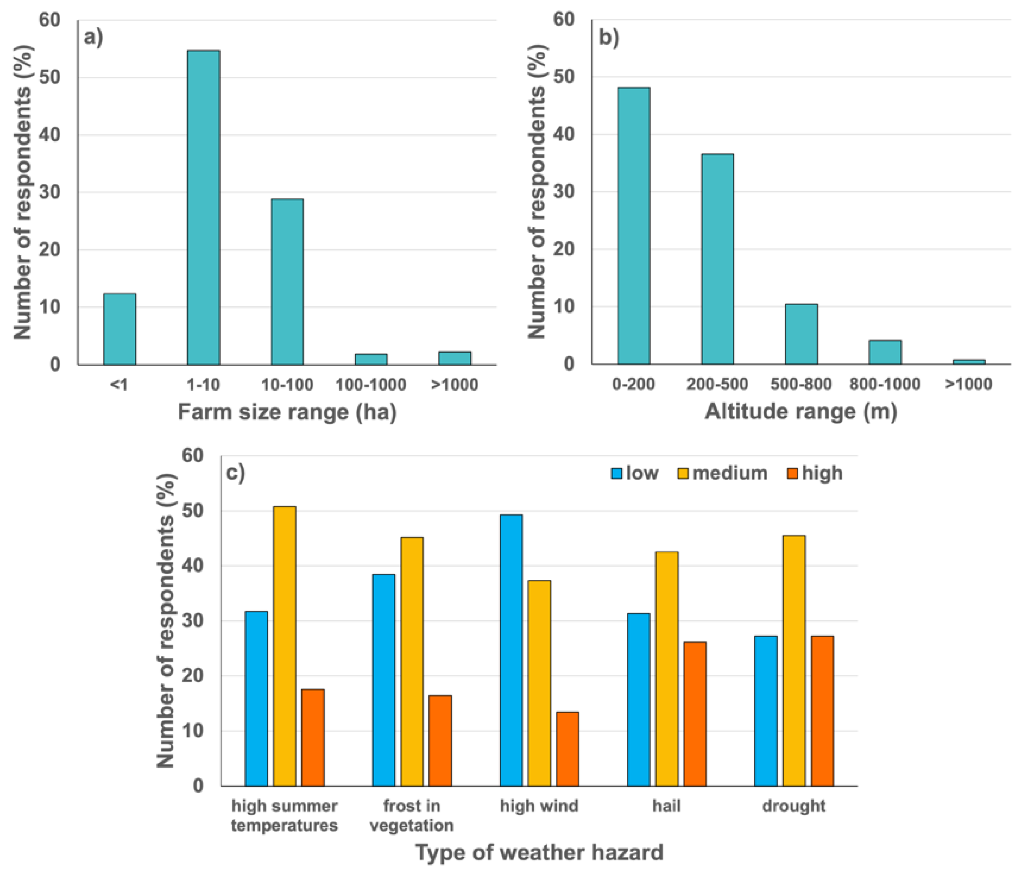
  • Surface area of farm;
  • Legal status of producer;
  • Altitude range of farm;
  • Type of production (annual crops, fruit, grapes, vegetables, etc.);
  • Five most represented varieties;
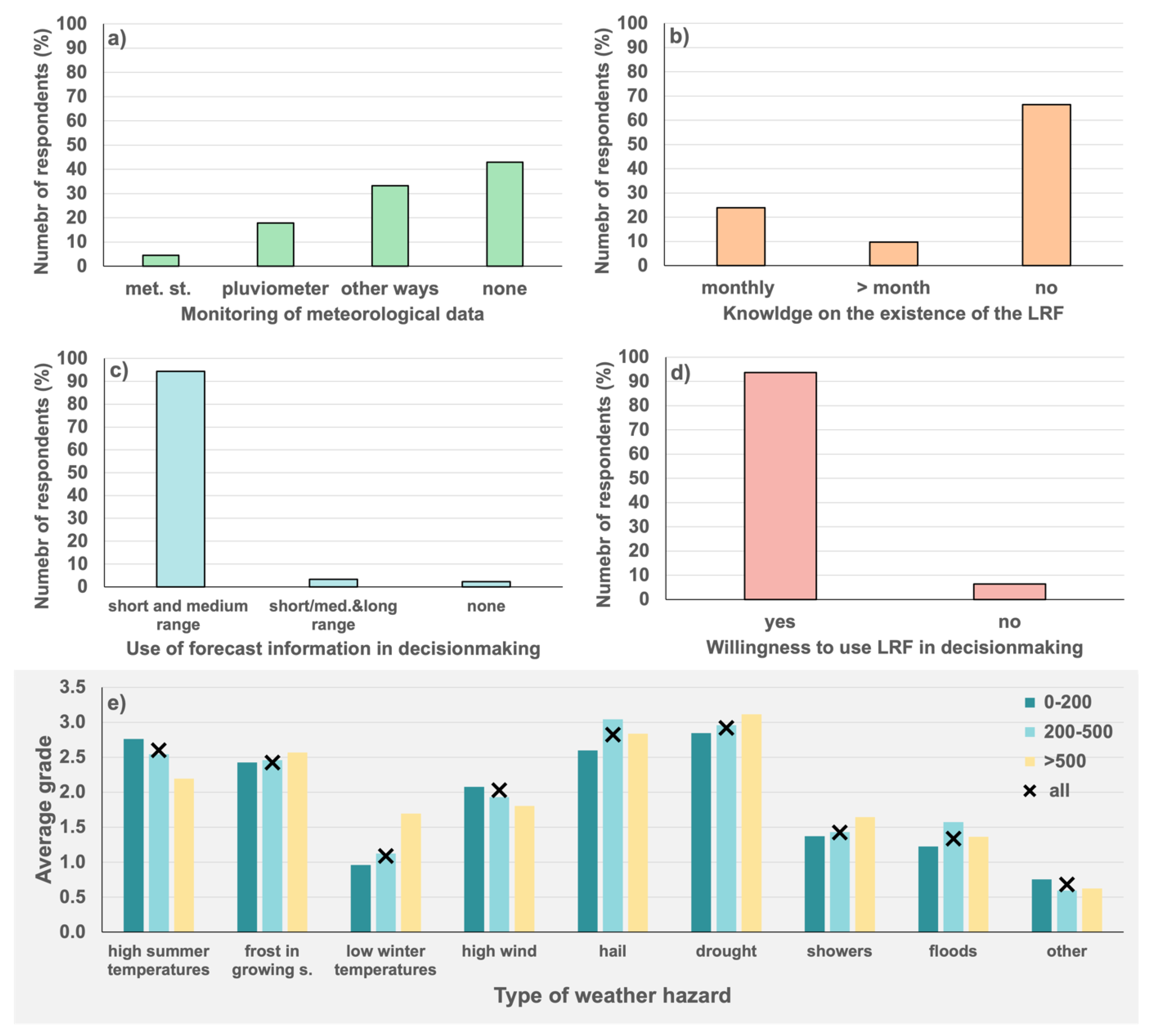
  • Grade for the level of damage (0–6) from: high summer temperatures, frost in the growing season, low winter temperatures, high wind/wind gusts, hail, drought, showers/extreme rain, floods and other extreme weather events (not listed);
  • Use and monitoring of meteorological measurements in production;
  • Knowledge about the existence of long range forecasts;
  • Implementation of forecast knowledge in the planning of production;
  • Media used for the retrieval of forecast information (TV, internet, etc.);
  • Source of weather forecasts (websites, applications, institutions, etc.);
  • Form of forecast that is most understandable (graphs, text, etc.);
  • Level of trust (1–10) in forecasts 1–2 days in advance;
  • Level of trust (1–10) in forecasts up to 7 days in advance;
  • Level of trust (1–10) in forecasts for one or more months in advance;
  • Level of usability (1–10) of forecasts 1–2 days in advance for planning production activities;
  • Level of usability (1–10) of forecasts up to 7 days in advance for planning production activities;
  • Level of usability (1–10) of forecasts for one or more months in advance for planning production activities;
  • Willingness to implement risk reduction measures according to information from seasonal forecasts; for example: if the forecast predicts that there is a 70% probability that an extreme weather event will occur during the growing season that could damage production, would the producer implement measures to reduce the risks (for annual crops change of variety or hybrid, change of crop rotation, reduction of surface with vulnerable crop; for perennial implementation of some protection measures, or nothing);
  • Additional comments on seasonal forecasts and their implementation in agricultural production planning.
The questionnaire was conducted in the period of February–March 2021. The weather conditions during the previous growing season did not involve significantly high summer temperatures or drought episodes, which could have affected the grading of the risks from the different types of weather hazards. The number of respondents was 268. The total surface area of their farms was 49,151.41 ha, which is about 1% of the total agricultural land in Serbia. The respondents were from all 24 counties in Serbia (without Kosovo). The distributions of the farm surface areas and the altitudes of the farms were presented in the main text. Out of the 268 respondents, 235 had family farms, 24 had legal entities and 8 classified their legal status as “other”.
The findings from the questionnaire which supplement the analysis in the main text are given in the Figure A1. General conclusion is that the respondents do not sufficiently coordinate their activities with weather conditions, probably because of the lack of knowledge how to do so and how to retrieve the needed information from the forecast data or to find the reliable source of the forecast information. Only 4% of the respondents had meteorological stations and 18% had pluviometers, but 43% did not perform any monitoring of weather conditions at their farms or in the vicinity (Figure A1a). Only 24% of the respondents were aware that the only form of LRFs that exists is monthly forecasts and 10% had heard about forecasts for longer periods, while the majority (66%) were not aware of the existence of long range forecasts (Figure A1b). It was highly likely that the respondents who knew about the monthly forecasts were informed by the daily newspaper Politika, which issues monthly forecasts for each day during the month at the beginning of each month. This forecast is made using a methodology in which analogies are found between current meteorological parameters and those from the past periods and are delivered as forecasts, based on similar cases that have been observed in the past. This approach is not eligible in the age of numerical weather prediction. For this reason, it was very likely that the producers were not well informed about monthly forecasts and had low expectations for the quality of long range forecasts.
Figure A1. The results from the questionnaire: the number of respondents (%) who monitored meteorological parameters (a); the number of respondents (%) who had knowledge about the existence of long range forecasts (b); the number of respondents (%) who used different types of forecasts (c); the number of respondents (%) who were willing to use long range forecast information if available in an understandable form (d); the distribution by altitude of average grades for the damages from different types of weather hazards with total average grade of damage (e).
Atmosphere 13 01337 g0a1
Over 90% of the respondents used the information from forecasts for up to 7 days in advance in their decision making (i.e., planning production activities), but only 3% also used the information from long range forecasts and 2% did not use any forecast information at all (Figure A1c). The respondents expressed a great interest (94%) in the use of long range forecast products (Figure A1d) if they were available and expressed in an understandable form, stating that it could help in their decision-making and in reducing the risks to production from extreme weather events.
Most importantly, the respondents assessed the level of damage (using grades 0–6) that had been caused to their production by different types of weather hazards (Figure A1e). The average grades were higher for high summer temperatures, frost in the growing season, high wind, hail and drought. Those hazards were further discussed in the main text. The highest grades were mostly in the range of 2–3 out of 6 because the respondents were a mixture of producers whose production had different vulnerabilities (depending on the crops that they grow). The grading according to the cultivated crops is not presented in this paper because most of the producers cultivated diverse crops on their farms, and they just provided a general assessment. To present the results more simply in the main text, the grades were categorized into the following levels of damage: “low” (grades 0 and 1), “medium” (grades 2, 3 and 4) and “high” (grades 5 and 6).

Appendix B. Supplement to the Long Range Forecast Analysis for Summer 2017

Here, we present the data that were used for the verification of the long range forecasts (LRFs) using the case study for the summer (June, July and August, JJA) of 2017 with the forecast run that started on 1 April 2017 (i.e., the leading month of the LRF was April). An assessment was conducted on the average JJA temperatures at 10 selected sites, for which regular meteorological measurements for the period of 1961–2020 were available. The locations and forecast assessment that was derived from these data were presented in the main text. Figure A2, Figure A3 and Figure A4 show the values for the average summer temperature at each station during the climate periods of 1961–1990 and 1991–2020, the observed average JJA temperatures for 2017 and the forecasted average JJA temperatures for 2017, respectively. As well as the average values, the minimum, 25th percentile, 75th percentile, and maximum values are also marked.
Figure A2. The average JJA values for the climate periods of 1961–1990 and 1991–2020, the average observed (obs) JJA value for 2017 and the median of the ensemble forecast (fcst) from April for the average JJA temperature for 2017 (red dots): the range of minimum to 25th percentile values is colored in light blue; range of 25th–75th percentile values is shaded in green; the range 75th percentile to maximum values is colored in light red; the values are given for Palic (upper left), Sremska Mitrovica (upper right), Smederevska Palanka (lower left) and Kraljevo (lower right).
Atmosphere 13 01337 g0a2
Figure A3. Same as Figure A2 but for Zajecar (upper left), Valjevo (upper right), Nis (lower left) and Vranje (lower right).
Atmosphere 13 01337 g0a3
Figure A4. Same as Figure A2 but for Zlatibor (left) and Sjenica (right).
Atmosphere 13 01337 g0a4

Appendix C. Supplement to the Long Range Forecast Analysis of the Prediction of Phenophases at the Plavinci Winery for 2017

Here, we present the data that supplemented our analysis of the quality of the long range forecasts (LRFs) for the case study at the Plavinci winery for the grapevine variety Panonia (white grape variety) in 2017.
To calculate the dates of the phenological phases (budburst, flowering, veraison and harvest), the growing degree days for each phenological stage were calculated. For budburst, the dates were calculated as the sixth day after the first occurrence of 5 consecutive days with average daily temperatures above 10 °C.
In Table A1, the dates that were derived from the ensemble LRFs that were initiated in March (leading month 3, LM03), April (LM04), May (LM05), June (LM06) and July (LM07) are presented. For the latter forecasts, for the period before the initialization of the forecast were used observed data and calculation continued with the predicted data after the initialization of the forecast.
Table A1. The observed (OBS) and predicted dates of budburst, flowering, veraison and harvest for the garpevine variety Panonia at the Plavinci winery in 2017; the predicted dates are presented for the ensemble LRFs that were initiated in March (LM03), April (LM04), May (LM05), June (LM06) and July (LM07); the results of the ensemble forecasts are presented as follows: minimum ensemble value (min), 25th percentile of ensemble values (p25), median (p50), 75th percentile of ensemble values (p75) and maximum ensemble value (max); the median (p50) was considered to be a representative ensemble value when compared to the observed values; note that the latter forecasts did not produce predicted dates for budburst and/or flowering because those phenophases occurred before the forecasts were initiated; the dates are presented as the “day of the year” and the observed values are also in the format of MM/DD.
OBS
Budburst 102 (4/12)
Flowering 143 (5/23)
Veraison 195 (7/14)
Harvest 234 (8/22)
LM03Minp25p50p75Max
Budburst102105107108112
Flowering133142145150158
Veraison182195199205214
Harvest225241248253277
LM04Minp25p50p75Max
Budburst102104105107113
Flowering128138141144155
Veraison180192196200215
Harvest216236243249285
LM05Minp25p50p75Max
Budburst
Flowering137143146149153
Veraison190197201204210
Harvest233241247252272
LM06Minp25p50p75Max
Budburst
Flowering
Veraison187196198201207
Harvest225237242245256
LM07Minp25p50p75Max
Budburst
Flowering
Veraison190194197199202
Harvest225236239242249
The predicted dates were relatively similar for all forecasts. Harvest dates were predicted to occur later than observed in all forecasts because of the decision of the producer to harvest the grapes when they had enough sugars for wine production, which was not necessarily at the time of physiological ripening, as mentioned in the main text. This decision was related to high temperatures during the harvest period, when the risk from drying of berries was high. One exception was the prediction of the harvest that was initiated in July, which predicted (according to the median value) the harvest only 5 days later the harvest date that was observed; however, the real harvest date was still below the 25th percentile value of this forecast, which confirmed that forecast bias (deviation from observation) was a consequence of producer intervention.
Table A2 shows the climate values of the dates of the phenophases for the case study location, which were derived from the temperature data using the same criteria as those in forecasts for their calculation. Since there were no long term meteorological observations for this site, the data were extracted from the high-resolution interpolated dataset that is available for up to 2017 in Serbia [29]. The difference in the average dates of the phenophases between the two climate periods demonstrated the large impact of increasing temperatures. During the climate period of 1961–1990, growing this grapevine variety was not possible because the heat conditions were suitable to reach harvest in only 6 out of the 30 years. During the 1991–2017 period, harvest was reached in 24 out of the 27 years. However, since this variety has only been grown at the Plavinci winery for the last decade (ending in 2021), the ripening was successful according to the producer statements. By comparing the observed dates for 2017 and the average (same as median) values that were derived from the climate period of 1991–2017, it was evident that the high temperatures in 2017 impacted early phenophase development, as was expected according to the climatology data. Budburst started 3 days later than expected, according to the average climate values, but flowering and veraison arrived early by 7 and 14 days, respectively. Harvest occurred 24 days before the climate average dates but, as mentioned before, this stage can be influenced by the producers’ decision to harvest the yield like in this case.
Table A2. The dates of budburst, flowering, veraison and harvest at the Plavinci winery for the climate periods 1991–1960 and 1991–2017, which were derived from interpolated temperature data; the values are given as the minimum (min), 25th percentile (p25), median (p50), 75th percentile (p75) and maximum (max) from the data for each year within the climate period.
Climate Period 1961–1990 (GDD Managed to Reach Harvest Date in Only 6 of 30 Years)
Minp25p50p75Max
Budburst8198109 (4/19)116127
Flowering145152158 (6/7)164171
Veraison212219224 (8/12)230248
Harvest272279292 (10/19)308331
Climate Period 1991–2017 (GDD Managed to Reach Harvest Date in 24 of 27 Years)
Minp25p50p75Max
Budburst809199 (4/9)107121
Flowering139146150 (5/30)156168
Veraison198204209 (7/28)214224
Harvest240252258 (9/15)273310

Appendix D. Supplement to the Analysis of Soil Moisture Seasonal Forecasts for 2017
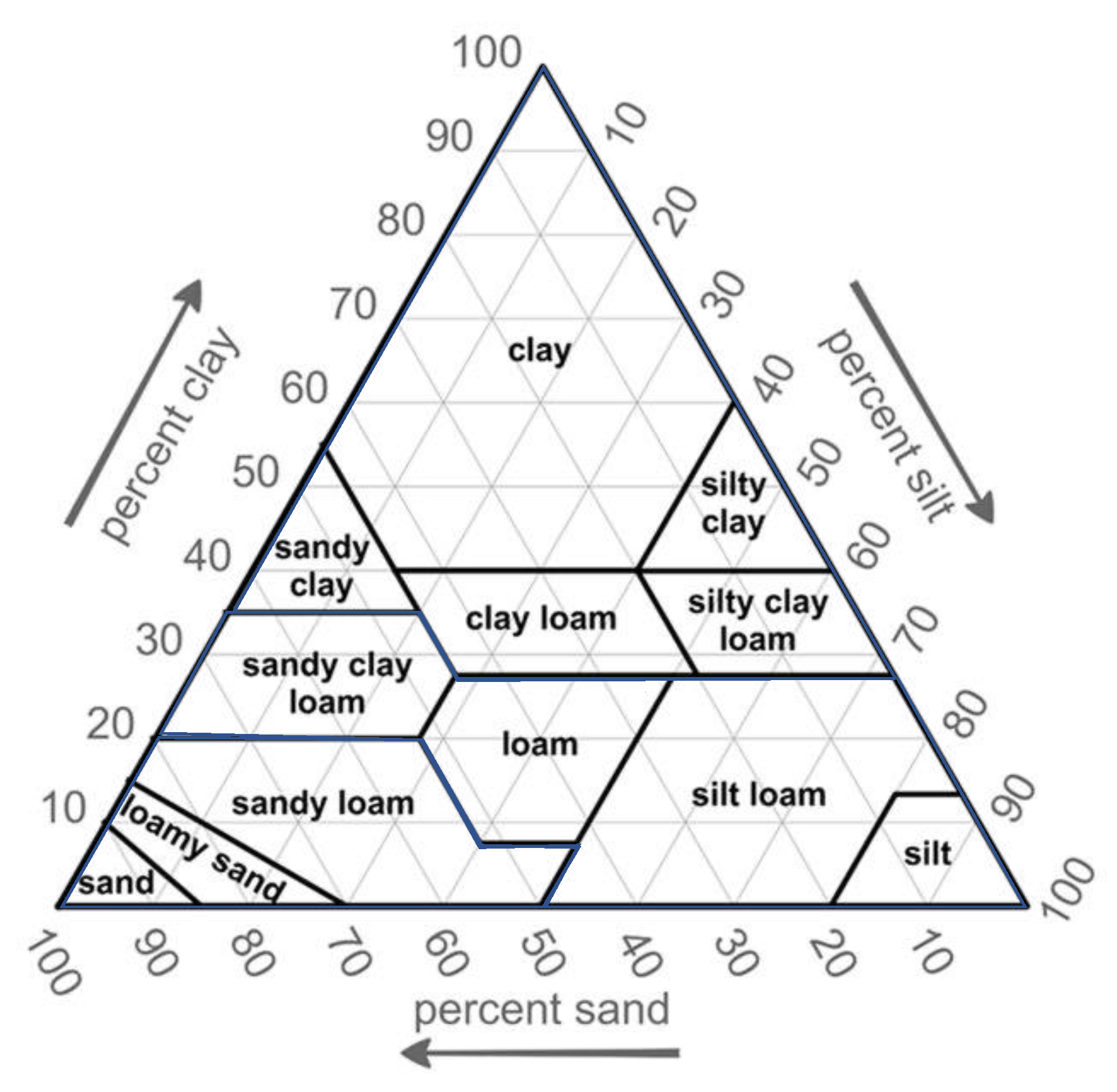
Soil moisture forecasts are used for long term forecasts (LRFs) for agricultural drought. An analysis was carried out for the forecasts that were initiated at the first day in March, April and May 2017. According to the SPEI6a (SPEI for a period of 6 months, ending with August), averaged for Serbia, 2017 was a year with drought (as discussed in the main text). During the period of March–August 2017, the average deficit of precipitation was almost 20% and the temperature anomaly was 2.5 °C compared to the values for the reference period 1961–1990.
In the numerical weather prediction model NMMB (which was used for the LRF), a NOAH land surface model was active for these simulations, in which soil types are divided into categories according to the USDA soil texture categorization and soil data from the STATSGO-FAO database were used. In Table A3, the most important parameters that are related to soil types are presented, which were extracted from the model. MAXSMC represents the maximum possible soil moisture for the given soil type. REFSMC represents the reference soil moisture (more commonly known as “field capacity”), which is the amount of the water in soil after excess water has drained away. WLTSMC represents the “wilting point”, which is the soil moisture at which the root extraction of water stops and the soil is considered to be a “dry soil”. Available water in the soil is with values of soil moisture content between wilting point and field capacity. As can be seen from Figure A5, the soil texture classes that contain the highest percentage of sand and the lowest percentage of clay have wilting point values below 0.05 m3m−3 and soils that have more clay have larger wilting point values, mostly above 0.1 m3m−3. So, soil with more clay reaches the dry condition at higher minimum soil moisture content. The reason for this is that it is harder for plants to extract the water from the soils with finer texture, and they reach wilting point at somewhat higher soil moisture content.
Table A3. The USDA soil types (soil texture) and related parameters as are defined in the model: in yellow are soils with wilting point below 0.05 m3m−3, in green larger than 0.05 m3m−3 and less than 0.1 m3m−3, and in blue with wilting points equal or above 0.1 m3m−3.
MAXSMCREFSMCWLTSMC
Sand0.3950.2360.023
Loamy Sand0.4210.2830.028
Sandy Loam0.4340.3120.047
Silty Loam0.4760.3600.084
Silt0.4760.3600.084
Loam0.4390.3290.066
Sandy Clay Loam0.4040.3150.069
Silty Clay Loam0.4640.3870.120
Clay Loam0.4650.3820.103
Sandy Clay0.4060.3380.100
Silty Clay0.4680.4040.126
Clay0.4570.4030.135
Figure A5. The USDA soil texture classification (as in Table A3) showing the clay, silt and clay contents in each category; the meaning of the colors is the same as in Table A3. (Figure adapted from the original that was authored by Derek G. Groenendyk, Ty P.A. Ferré, Kelly R. Thorp and Amy K. Rice, named the “USDA Soil Texture Triangle”).
Atmosphere 13 01337 g0a5
According to the soil-related parameters in the model, it is possible for dry soil conditions (no available water for plants) to be reached when the values are below 0.15 m3m−3, depending on the soil texture (soil type). Different plants have different demands for water and the model only recognizes a limited number of land cover types (cropland, pasture, two types of forest, water, bare, etc.). So, there is no division between cropland plants. In the land surface model, which is part of the numerical weather prediction models, all relevant heat- and water-related processes were included, but it is not possible to include fully accurate information on the real land cover and soil characteristics in the model. Nonetheless, the sensitivity of the forecasts was not significant to this approximate representation of the land surface characteristics, especially in the prediction of weather conditions over longer periods, such as droughts. This is valid in in case the categories of land covers and soil textures are not completely inaccurate.
For this case study, since the target was the prediction of agricultural droughts months in advance, we hypothesized that when soil moisture drops below 0.15 m3m−3, the soil is dry if it contains a significant portion of clay. If the values are below 0.1 m3m−3, and especially below 0.05 m3m−3, for soils that have less clay, the soil is dry. The details about soil texture and land cover seen by the model at the selected locations were not considered (though it was possible) since it was not of the significance for this work and is more in the domain of the verification of the model itself and not the verification of the usability of its results.
The average soil moisture values were presented in the main text. Figure A6, Figure A7, Figure A8, Figure A9, Figure A10, Figure A11, Figure A12, Figure A13, Figure A14 and Figure A15 show the results obtained for each location separately. The results are presented for three depths (10 cm, 30 cm and 60 cm) and from three LRFs (those that were initiated in March, April and May). The values are of the forecast ensemble median, which is considered as the most probable forecasted value.
Figure A6. The ensemble medians of the 10-day running averages of soil moisture content (wg, in m3m−3) at different depths at Palic (pal), obtained from forecasts that were initiated in March (a), April (b) and May (c) 2017.
Atmosphere 13 01337 g0a6
Figure A7. The ensemble medians of the 10-days moving averages of soil moisture content (wg, in m3m−3) at different depths at Sremska Mitrovica (srm), obtained from forecasts that were initiated in March (a), April (b) and May (c) 2017.
Atmosphere 13 01337 g0a7
Figure A8. The ensemble medians of the 10-day moving averages of soil moisture content (wg, in m3m−3) at different depths at Smederevska Palanka (smp), obtained from forecasts that were initiated in March (a), April (b) and May (c) 2017.
Atmosphere 13 01337 g0a8
Figure A9. The ensemble medians of the 10-day moving averages of soil moisture content (wg, in m3m−3) at different depths at Kraljevo (kra), obtained from forecasts that were initiated in March (a), April (b) and May (c) 2017.
Atmosphere 13 01337 g0a9
Figure A10. The ensemble medians of the 10-day moving averages of soil moisture content (wg, in m3m−3) at different depths at Zajecar (zaj), obtained from forecasts that were initiated in March (a), April (b) and May (c) 2017.
Atmosphere 13 01337 g0a10
Figure A11. The ensemble medians of the 10-day moving averages of soil moisture content (wg, in m3m−3) at different depths at Valjevo (vlj), obtained from forecasts that were initiated in March (a), April (b) and May (c) 2017.
Atmosphere 13 01337 g0a11
Figure A12. The ensemble medians of the 10-day moving averages of soil moisture content (wg, in m3m−3) at different depths at Nis (nis), obtained from forecasts that were initiated in March (a), April (b) and May (c) 2017.
Atmosphere 13 01337 g0a12
Figure A13. The ensemble medians of the 10-day moving averages of soil moisture content (wg, in m3m−3) at different depths at Vranje (vra), obtained from forecasts that were initiated in March (a), April (b) and May (c) 2017.
Atmosphere 13 01337 g0a13
Figure A14. The ensemble medians of the 10-day moving averages of soil moisture content (wg, in m3m−3) at different depths at Zlatibor (zla), obtained from forecasts that were initiated in March (a), April (b) and May (c) 2017.
Atmosphere 13 01337 g0a14
Figure A15. The ensemble medians of the 10-day moving averages of soil moisture content (wg, in m3m−3) at different depths at Sjenica (sje), obtained from forecasts that were initiated in March (a), April (b) and May (c) 2017.
Atmosphere 13 01337 g0a15
The main conclusions from these results are:
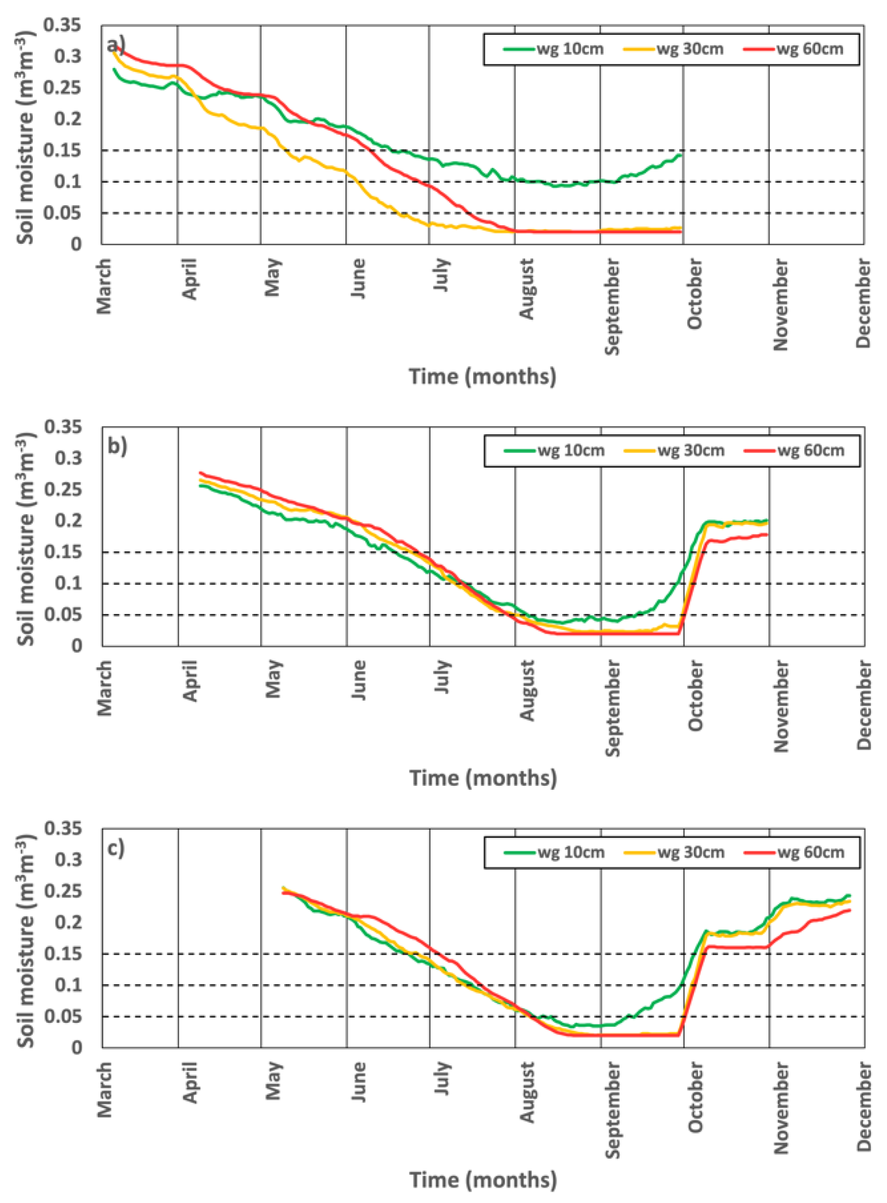
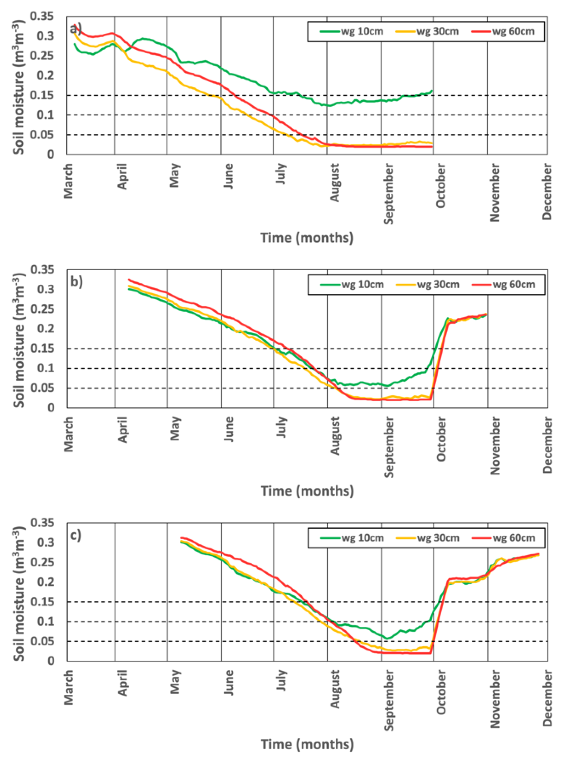
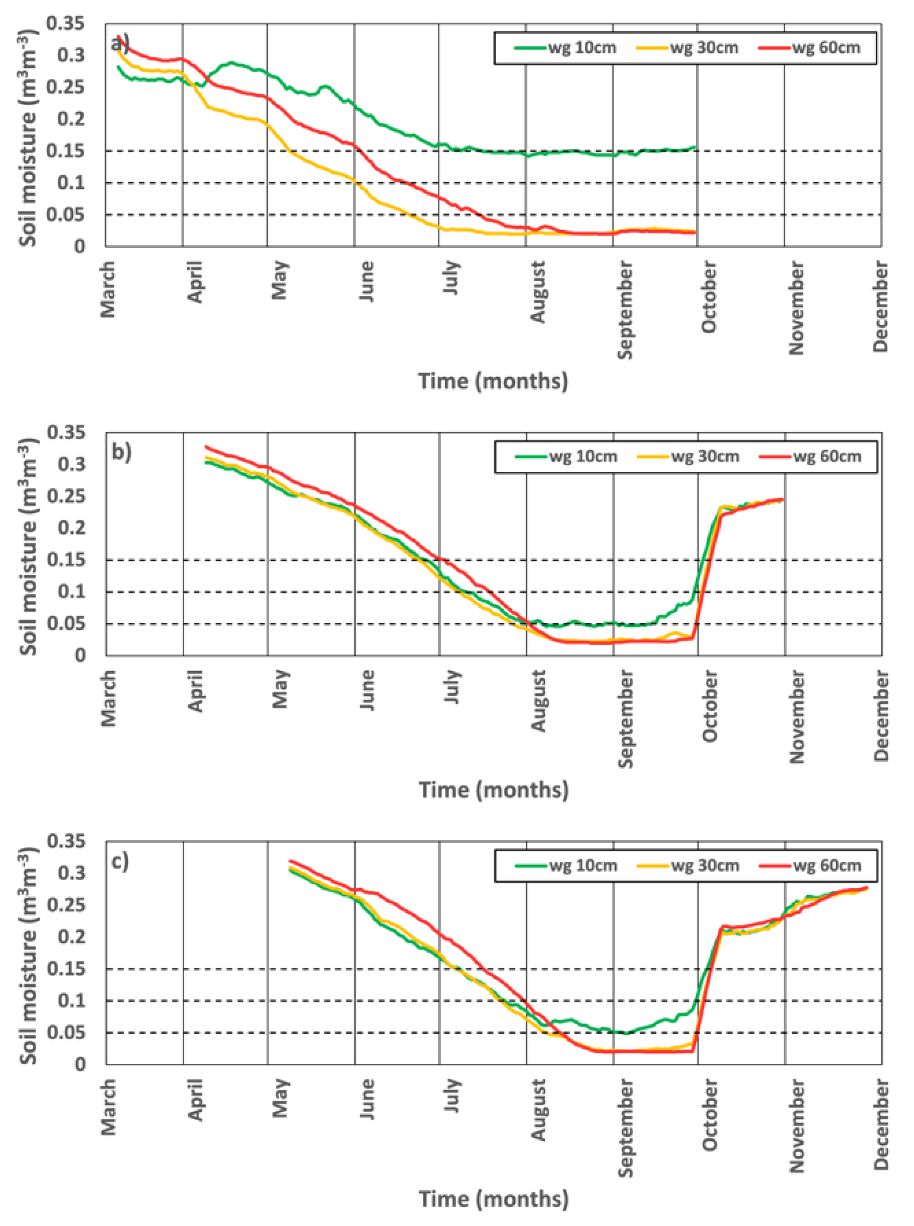
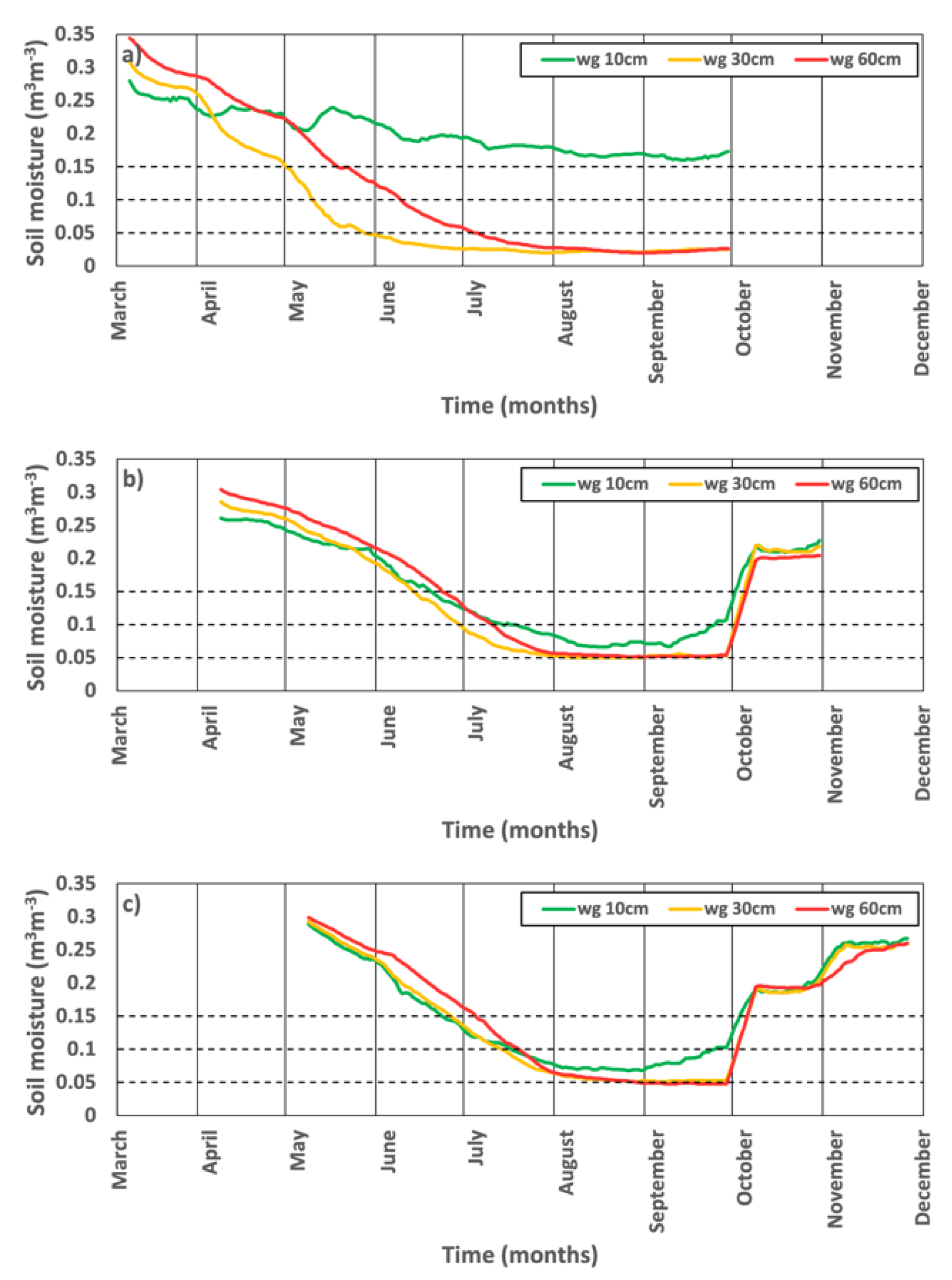
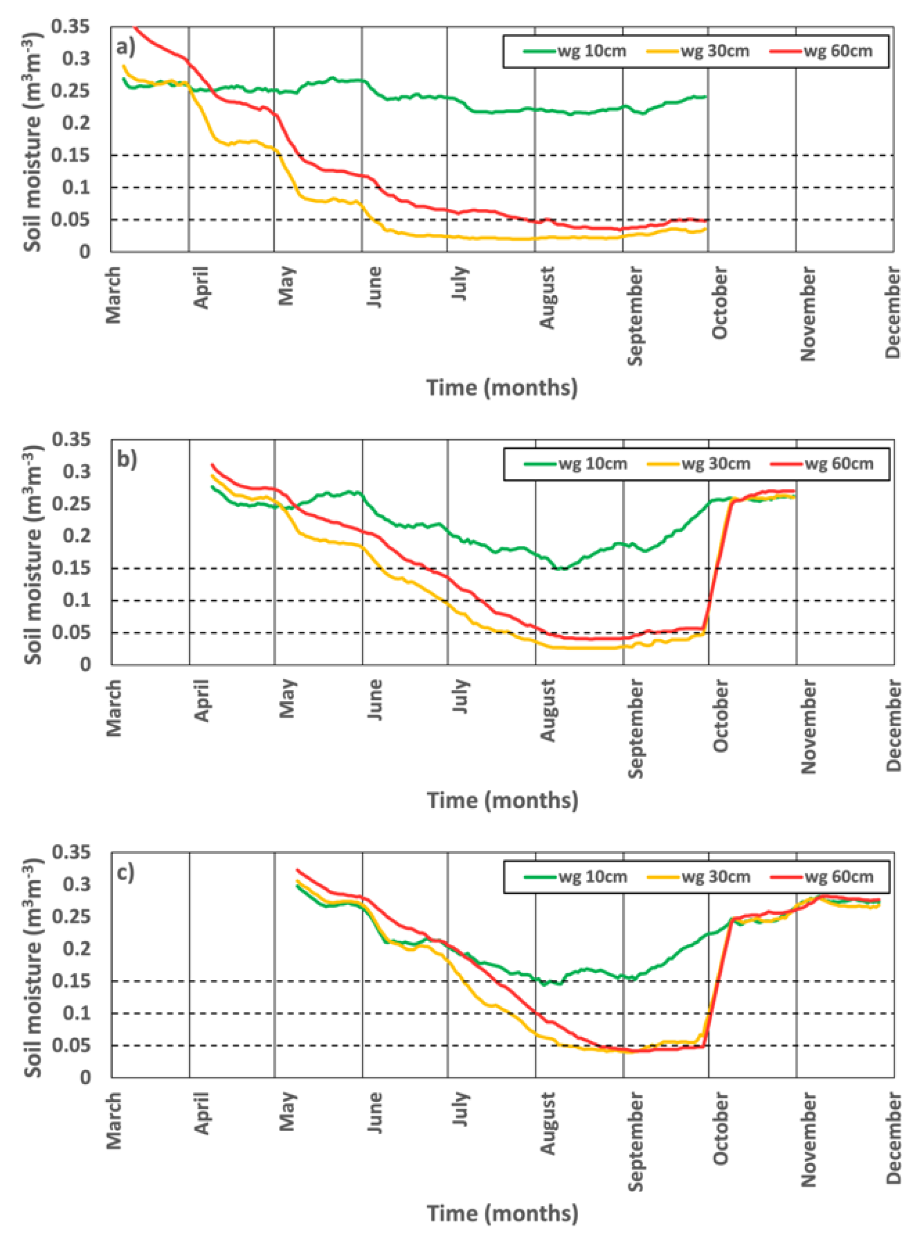
  • Dry soil was forecasted at eight of the ten locations;
  • Soil moisture reached its minimum possible value (no available water) in deeper soil (30 cm and 60 cm) at most locations, but at some locations also in shallow parts;
  • The major root mass of the cultivars is in deeper soil and, therefore, the deeper soil forecasts are more relevant, which means that the drought forecasts produced by using the long term prediction of soil moisture is a good approach;
  • In the latter forecasts, the onset of dry conditions was predicted to occur later, possibly due to the spin-up of the soil conditions in the model because the initial soil moisture conditions were not appropriate and probably overestimated, which means that the model needed time to adjust the soil conditions to the weather conditions; for this reason, it is better for the prediction of soil moisture to use forecasts that are initiated earlier.
We were not able to perform quantified verifications at the selected locations because there were no soil moisture measurements available.

References

  1. Vuković, A.; Vujadinović Mandić, M. Study on Climate Change in the Western Balkans Region; Regional Cooperation Council Secretariat: Sarajevo, Bosnia and Herzegovina, 2018; p. 76. ISBN 978-9926-402-09-9. [Google Scholar]
  2. Vukovic, A.; Vujadinovic, M.; Rendulic, S.; Djurdjevic, V.; Ruml, M.; Babic, V.; Popovic, D. Global warming impact on climate change in Serbia for the period 1961–2100. Therm. Sci. 2018, 22, 2267–2280. [Google Scholar] [CrossRef]
  3. Đurdjević, V.; Vuković, A.; Vujadinović Mandić, M. Observed Climate Change in Serbia and Projections of Future Climate Based on Different Scenarios of Future Emissions; United Nation’s Development Program: Belgrade, Serbia, 2018; p. 24. (In Serbian) [Google Scholar]
  4. Stričević, R.; Prodanović, S.; Đurović, N.; Petrović Obradović, O.; Đurović, D. Climate Change Impacts on Serbian Agriculture; United Nation’s Development Program: Belgrade, Serbia, 2019; p. 52. [Google Scholar]
  5. Stričević, R.; Lipovac, A.; Prodanović, S.; Ristovski, M.; Petrović Obradović, O.; Djurović, N.; Djurović, D. Vulnerability of agriculture to climate change in Serbia–Farmer’s assessment of impacts and damages. J. Agric. Sci. 2020, 65, 263–281. [Google Scholar]
  6. Revision of the Nationally Determined Contributions of Republic of Serbia for Paris Agreement–Climate Change Adaptation. Available online: https://www.klimatskepromene.rs/wp-content/uploads/2020/10/CCA-revised-NDCs-DRAFT-OCT-2020.pdf (accessed on 31 July 2022).
  7. Đurđević, V. Drought Initiative–Republic of Serbia, UNCCD. Available online: https://www.unccd.int/sites/default/files/country_profile_documents/NDP_SERBIA_2020.pdf (accessed on 31 July 2022).
  8. Vujadinović Mandić, M.; Ranković-Vasić, Z.; Ćosić, M.; Simić, A.; Đurivić, D.; Dolijanović, Ž.; Vuković Vimić, A.; Životić, L.; Stanojević, D.; Lipovac, A. Report on the Impact of Climate Change on the Agriculture Sector, with Proposed Adaptation Measures. Activity 3: Proposed Adaptation Measures. Available online: https://adaptacije.klimatskepromene.rs/wp-content/uploads/2022/03/Agriculture-3.-Proposed-adaptation-measures.pdf (accessed on 31 July 2022).
  9. Calanca, P.; Bolius, D.; Weigel, A.; Liniger, M. Application of Long-Range Weather Forecasts to Agricultural Decision Problems in Europe. J. Agric. Sci. 2011, 149, 15–22. [Google Scholar] [CrossRef] [Green Version]
  10. Gunda, T.; Bazuin, J.T.; Nay, J.; Yeung, K.L. Impact of seasonal forecast use on agricultural income in a system with varying crop costs and returns: An empirically-grounded simulation. Environ. Res. Lett. 2017, 12, 034001. [Google Scholar] [CrossRef] [Green Version]
  11. Manzanas, R.; Gutiérrez, J.M.; Fernández, J.; van Meijgaard, E.; Calmanti, S.; Magariño, M.E.; Cofiño, A.S.; Herrera, S. Dynamical and statistical downscaling of seasonal temperature forecasts in Europe: Added value for user applications. Clim. Serv. 2018, 9, 44–56. [Google Scholar] [CrossRef]
  12. Nikulin, G.; Asharaf, S.; Magariño, M.E.; Calmanti, S.; Cardoso, R.M.; Bhend, J.; Fernández, J.; Frías, M.D.; Fröhlich, K.; Früh, B.; et al. Dynamical and statistical downscaling of a global seasonal hindcast in eastern Africa. Clim. Serv. 2018, 9, 72–85. [Google Scholar] [CrossRef]
  13. Gregow, H.; Lehtonen, I.; Pirinen, P.; Venäläinen, A.; Vajda, A.; Koskiniemi, J. Preparing for peat production seasons in Finland and experimenting with long range impact forecasting. Clim. Serv. 2019, 14, 37–50. [Google Scholar] [CrossRef]
  14. Iizumi, T.; Shin, Y.; Kim, W.; Kim, M.; Choi, J. Global crop yield forecasting using seasonal climate information from a multi-model ensemble. Clim. Serv. 2018, 11, 13–23. [Google Scholar] [CrossRef]
  15. Streefkerk, I.N.; van den Homberg, M.J.C.; Whitfield, S.; Mittal, N.; Pope, E.; Werner, M.; Winsemius, H.C.; Comes, T.; Ertsen, M.W. Contextualising seasonal climate forecasts by integrating local knowledge on drought in Malawi. Clim. Serv. 2022, 25, 100268. [Google Scholar] [CrossRef]
  16. Kumar, P.; Shah, S.F.; Uqaili, M.A.; Kumar, L.; Zafar, R.F. Forecasting of Drought: A Case Study of Water-Stressed Region of Pakistan. Atmosphere 2021, 12, 1248. [Google Scholar] [CrossRef]
  17. Miller, S.; Mishra, V.; Ellenburg, W.L.; Adams, E.; Roberts, J.; Limaye, A.; Griffin, R. Analysis of a Short-Term and a Seasonal Precipitation Forecast over Kenya. Atmosphere 2021, 12, 1371. [Google Scholar] [CrossRef]
  18. Cowan, T.; Stone, R.; Wheeler, M.C.; Griffiths, M. Improving the seasonal prediction of Northern Australian rainfall onset to help with grazing management decisions. Clim. Serv. 2020, 19, 100182. [Google Scholar] [CrossRef]
  19. Gbangou, T.; Ludwig, F.; van Slobbe, E.; Hoang, L.; Kranjac-Berisavljevic, G. Seasonal variability and predictability of agro-meteorological indices: Tailoring onset of rainy season estimation to meet farmers’ needs in Ghana. Clim. Serv. 2019, 14, 19–30. [Google Scholar] [CrossRef]
  20. Ceglar, A.; Toreti, A. Seasonal climate forecast can inform the European agricultural sector well in advance of harvesting. NPJ Clim. Atmos. Sci. 2021, 4, 42. [Google Scholar] [CrossRef]
  21. Bedia, J.; Golding, N.; Casanueva, A.; Iturbide, M.; Buontempo, C.; Gutiérrez, J.M. Seasonal predictions of Fire Weather Index: Paving the way for their operational applicability in Mediterranean Europe. Clim. Serv. 2018, 9, 101–110. [Google Scholar] [CrossRef]
  22. Pope, E.C.D.; Buontempo, C.; Economou, T. Exploring constraints on the realised value of a forecast-based climate service. Clim. Serv. 2019, 15, 100102. [Google Scholar] [CrossRef]
  23. Vaughan, C.; Muth, M.F.; Brown, D.P. Evaluation of regional climate services: Learning from seasonal-scale examples across the Americas. Clim. Serv. 2019, 15, 100104. [Google Scholar] [CrossRef]
  24. An-Vo, D.-A.; Radanielson, A.M.; Mushtaq, S.; Reardon-Smith, K.; Hewitt, C. A framework for assessing the value of seasonal climate forecasting in key agricultural decisions. Clim. Serv. 2021, 22, 100234. [Google Scholar] [CrossRef]
  25. Born, L.; Prager, S.; Ramirez-Villegas, J.; Imbach, P. A global meta-analysis of climate services and decision-making in agriculture. Clim. Serv. 2021, 22, 100231. [Google Scholar] [CrossRef]
  26. Djurdjevic, V.; Janjic, Z.; Pejanovic, G.; Vasic, R.; Rajkovic, B.; Djordjevic, M.; Vujadinovic, M.; Vukovic, A.; Lompar, M. NCEP’s multi-scale NMMB model in the Hydrometeorological Service of Serbia: Experiences and recent model developments. In EGU General Assembly, Geophysical Research Abstracts; EGU2013-8217; EGU General Assembly: Vienna, Austria, 2013; Volume 15. [Google Scholar]
  27. Janjic, Z.; Gall, R.L. Scientific documentation of the NCEP nonhydrostatic multiscale model on the B grid (NMMB). Part 1 Dynamics (No. NCAR/TN-489+STR). Univ. Corp. Atmos. Res. 2012. [Google Scholar] [CrossRef]
  28. Haylock, M.R.; Hofstra, N.; Klein Tank, A.M.G.; Klok, E.J.; Jones, P.D.; New, M. A European Daily High-Resolution Gridded Data Set of Surface Temperature and Precipitation for 1950–2006. J. Geophys. Res. 2008, 113, D20119. [Google Scholar] [CrossRef] [Green Version]
  29. Vujadinović Mandić, M.; Vuković Vimić, A.; Ranković-Vasić, Z.; Đurović, D.; Ćosić, M.; Sotonica, D.; Nikolić, D.; Đurđević, V. Observed Changes in Climate Conditions and Weather-Related Risks in Fruit and Grape Production in Serbia. Atmosphere 2022, 13, 948. [Google Scholar] [CrossRef]
  30. Vujadinović Mandić, M.; Ranković-Vasić, Z.; Ćosić, M.; Simić, A.; Đurivić, D.; Dolijanović, Ž.; Vuković Vimić, A.; Životić, L.; Stanojević, D.; Lipovac, A. Report on the Impact of Climate Change on the Agriculture Sector, with Proposed Adaptation Measures. Activity 1: Risk and Vulnerability Assessment–Observed: Occurrences, Impacts, and Levels of Affectedness within. Available online: https://adaptacije.klimatskepromene.rs/wp-content/uploads/2022/03/Agriculture-1.-Risk-and-Vulnerability-assessment.pdf (accessed on 31 July 2022).
  31. Vujadinović Mandić, M.; Ranković-Vasić, Z.; Ćosić, M.; Simić, A.; Đurivić, D.; Dolijanović, Ž.; Vuković Vimić, A.; Životić, L.; Stanojević, D.; Lipovac, A. Report on the Impact of Climate Change on the Agriculture Sector, with Proposed Adaptation Measures. Activity 2: Assessing the Impact of Climate Change on the Agricultural Sector in the Future. Available online: https://adaptacije.klimatskepromene.rs/wp-content/uploads/2022/03/Agriculture-2.-Assessing-climate-change-in-teh-future.pdf (accessed on 31 July 2022).
  32. Životić, L.; Vuković Vimić, A. Soil Degradation and Climate Change in Serbia; United Nation’s Development Program: Belgrade, Serbia, 2022; p. 24. ISBN 978-86-7728-356-8. [Google Scholar]
  33. Beguería, S.; Vicente-Serrano, S.M.; Reig, F.; Latorre, B. Standardized precipitation evapotranspiration index (SPEI) revisited: Parameter fitting, evapotranspiration models, tools, datasets and drought monitoring. Int. J. Climatol. 2013, 34, 3001–3023. [Google Scholar] [CrossRef] [Green Version]
  34. Esit, M.; Kumar, S.; Pandey, A.; Lawrence, D.M.; Rangwala, I.; Yeager, S. Seasonal to multi-year soil moisture drought forecasting. NPJ Clim. Atmos. Sci. 2021, 4, 16. [Google Scholar] [CrossRef]
  35. Vuković Vimić, A.; Vujadinović Mandić, M.; Đurđević, V.; Ranković-Vasić, Z.; Ćosić, M.; Nikolić, D. Seasonal Forecast and Agricultural Production. In Proceedings of the Seasonal Forecast and Adaptation of Agriculture to Climate Change, Belgrade, Serbia, 19 May 2022; ISBN 978-86-7834-400-8. [Google Scholar]
Figure 1. The location of the Republic of Serbia in Europe (marked in orange) and the domain for long range forecasts (marked with the blue line) (a) and the topography of the Serbian territory and locations with observed meteorological data (in blue) and phenology data (in red) (b).
Atmosphere 13 01337 g001
Figure 2. A schematic diagram of the IAPS project activities.
Atmosphere 13 01337 g002
Figure 3. Mean monthly values, averaged for the territory of Serbia, for temperature (a) and accumulated precipitation (b) for the period 2011–2020 (in orange) and for the reference period 1961–1990 (in grey).
Atmosphere 13 01337 g003
Figure 4. The SPEI6a values for the period of March–August (a) and anomalies with respect to the values for the period of 1961–1990 for the average temperature (b) and the average accumulated precipitation (c) for the period March-August for each year in 1961–2020; in black are marked values for the years with drought in the reference period 1961–1990 and in red are marked values for years with drought in the period 2011–2020; blue dashed line is a linear trend; years with drought the ones with SPEI6a lower than −1.
Atmosphere 13 01337 g004
Figure 5. Information from the questionnaire that was conducted among agricultural producers: the distribution of the farm size of the respondents (a); the distribution of the altitudes of the respondents’ farms (b); the distributions of the levels of risk of the different types of hazards for production, as assessed by the respondents (c).
Atmosphere 13 01337 g005
Figure 6. The range of values lesser or equal to minimum value, between minimum and 25th percentile, between 25th and 75th percentile, between 75th percentile and maximum value, and higher or equal to maximum value) in which the observed value for the average summer temperature in 2017 fits: for: climate period 1961–1990 (x), climate period 1991–2020 (+), ensemble of long range forecast for 2017 initiated at 1 April 2017 (o); sign minus (−) imply that the forecasted anomaly was opposite than the observed, compared to the average values for the climate period 1961–1990; forecast skill is given for each station according to the criteria given in the text.
Atmosphere 13 01337 g006
Figure 8. Soil moisture (m3m−3) 10-day running average, averaged for 8 locations (at lower altitudes), for 2017, from the forecast initiated on 1 April 2017, at 10 cm depth (a), 30 cm (b) and 60 cm (c); values are given for the ensemble forecast median values (darker colors) and for the 25th and 75th percentile (lighter colors); dashed lines represent threshold for dry soil for different soil types, as explained in the text and in Appendix D.
Atmosphere 13 01337 g008
Table 1. A list of the locations of the meteorological observations and phenology data (last row): Acr., acronym; Long., longitude; Lat., latitude; Alt., altitude. The locations are also presented in Figure 1.
Acr.Long. (°)Lat. (°)Alt. (m)Name
pal46.1019.77102Palic
srm44.9719.6381Sremska Mitrovica
smp44.3720.95122Smederevska Palanka
vlj44.2819.92176Valjevo
kra43.7220.70215Kraljevo
nis43.3321.87197Nis
vra42.4821.90432Vranje
zaj43.8822.28144Zajecar
zla43.7319.721028Zlatibor
sje43.2720.021038Sjenica
PLA44.7020.69170Plavinci Winery
Publisher’s Note: MDPI stays neutral with regard to jurisdictional claims in published maps and institutional affiliations.

