Assessment of Temperature and Precipitation Forecasts of the WRF Model in the Bahía de Banderas Region (Mexico)

Abstract

The Centro de Ciencias de la Atmósfera at UNAM, in Mexico, uses the Water Research and Forecasting model to provide weather forecasts to the country. In this study, we downloaded the mean temperature and precipitation forecasts of the first 24 h generated by the WRF model in the center of the country. Only the time series of our study region (Bahía de Banderas) was processed from this database, from June to October 2010, and these data were compared with the data recorded in six stations to evaluate the performance of the model at a local level. Data from 12 stations were used to construct the observed temperature and precipitation maps for spatial validation. The results show that the model performance was partially acceptable. The correlation coefficient for hourly temperatures was an average of $r=0.84$. Errors were less than $2 °\mathrm{C}$ with a BIAS of $\pm 1 °\mathrm{C}$. For the accumulated 24 h precipitation, however, the results were not satisfactory $\left(r=0.26\right)$. The model predicted only 25.7% of the rainy days observed. In terms of spatial distribution, $~2.3$ times more rain was observed than had been predicted by the model.

1. Introduction

Precipitation is an important element in the Earth’s hydrological cycle and is dynamically linked to atmospheric circulation, redistributing latent heat throughout the troposphere [1].

The hydrometeorological phenomena that occur in Mexico directly affect the primary activities of its economy (agriculture, fishing, forestry, livestock, and mining) and its urban and rural populations [2,3,4]. In general, flood risk depends more on vulnerability, due to the poor urban planning of infrastructure exposed to meteorological phenomena [5]. Meanwhile, the amount of economic damage due to floods in primary activities is lower than in urban areas for the same level of exposure [4,6]. Forecasting is essential to prevent risk in the economic activities and urban sector [7].

Forecasting the weather can be carried out based on the analysis of synoptic maps, upper air data, satellite and radar images, and statistical analysis, to computational modeling [8,9]. Such studies promote numerical weather forecasting, leading to the development of atmospheric prediction models [7]. Numerical weather prediction (NWP) models, as a complement to the interpretation of conventional observations, can increase the certainty of the forecasting process [3]. There are three forecasting models: global, regional, and mesoscale [8,10]. In global modeling, most precipitation forecasts based on global NWP models are available at large spatial scales (28 km, GFS) [11]. Meanwhile, regional numerical weather prediction models can reproduce small-scale (20 km) phenomena, such as storms [8,11]. Mesoscale models can provide resolutions down to a few kilometers (2 km) [8]. A higher spatial and temporal resolution in the NWP model allows the evolution of a meteorological phenomenon to be observed in greater detail and thus provides a more detailed framework in which the actual observations can be interpreted [3,12].

Weather research and forecasting (WRF) is an atmospheric model designed for both research and numerical weather prediction [13]. The WRF model was the result of a multi-agency effort to provide a next-generation system for mesoscale forecast modeling [3].

Corrales et al. [3] evaluated the amount of rain accumulated by 24 h predicted in the WRF model in Mexico and compared it with the data registered in the Automated Stations National Network managed by the Instituto Nacional de Investigaciones Forestales, Agrícolas y Pecuarias (INIFAP, Mexico City, Mexico), from July 2012 to February 2013. They integrated the model at 120 h and configured a single domain with 13 km of mesh pitch and a 35-level vertical structure. However, the precipitation forecast given by the WRF model was not statistically significant to its study [3].

The present research focused on the Bahía de Banderas region (BB), located in the central zone of the western coast of Mexico, which has great tourist, ecological and economic importance at the national level. In addition, adequate and reliable spatial forecasts of precipitation and temperature are of interest in this region, due to the impact of these meteorological events in the agricultural areas of the Ameca River Valley, Tomatlán, and Talpa de Allende (Figure 1), as well as the problems of flooding in urban areas or the effect of landslides on highways. So far, no numerical model can produce a perfect weather forecast, since there are different error sources, so it is essential to verify predicted variables by comparing them with observations through the use of statistical parameters [14].

The study period (from June to October 2010) was chosen for two large atypical phenomena that occurred in the BB region. One of these phenomena was caused by a tropical wave associated with the trade winds from the NE, which caused atmospheric instability in the whole region and generated a series of storms in the Ameca River basin, Mexico. This caused this river to overflow, destroying one of the most important bridges in the city. Later, atypical storms (>100 mm) appeared in the region, which caused severe flooding and runoff in urban and rural areas. One of the objectives of this research was to determine the efficiency of the WRF model to forecast atypical events such as those mentioned. In addition, this study also evaluated the temperature and precipitation forecasts generated by the WRF model (resolution of 7 km) and compared them with the real data recorded in the atmospheric monitoring network in the BB region. This was to determine the degree of confidence that can be obtained in weather forecasts at the local level.

2. Materials and Methods

2.1. Study Area

The BB region is located in the Jalisco Block [15], at 19°54′–21°00′ N and 104°00′–105°46′ W, and occupies 11,133 km² of the area on the mainland [16]. It is part of the coastal plain of the Mexican Pacific and has mountains reaching 2600 m above sea level, which gives it a very rugged topography, particularly in the central and eastern areas (Figure 1). Watercourses from these mountains carry rainwater down the Ameca River Valley, through the city of Puerto Vallarta, and into Banderas Bay. The Cacoma and El Tuito mountain ranges are natural hydrological frontiers that partially drain precipitation to the south, generated by the weather systems that arrive from the south and southeast [16,17].

Figure 1. Digital elevation model in 3D [18]. Significant topographic features are indicated with black capital letters: (A) Vallejo Mountain; (B) La Cumbre Hill; (C) Ameca River Valley; (D) Puerto Vallarta City; (E) Pitillal River; (F) La Bufa Hill; (G) Cuale River; (H) Jolapa Mountains; (I) Talpa de Allende City; (J) El Cuale Mountain; (K) El Tuito Mountain; (L) Cacoma Mountain; (M) Cajón Peña Dam; (N) Tomatlán City; (O) Banderas Bay. The stations used for 24-h validation are indicated with red triangles: (1) Tec Ny; (2) Asfalto; (3) CUC; (4) Prepa PV; (5) Coapinole; (6) Tomatlán River; and the black triangles indicated the stations used for the spatial validation: (7) Monteón; (8) Valle de Banderas; (9) San Juan; (10) La Desembocada; (11) Cajón Peña; (12) El Bramador; (13) El Tuito; (14) Talpa; (15) Mascota; (16) Corrinchis; (17) Mixtlán; (18) San Gregorio.

Figure 1. Digital elevation model in 3D [18]. Significant topographic features are indicated with black capital letters: (A) Vallejo Mountain; (B) La Cumbre Hill; (C) Ameca River Valley; (D) Puerto Vallarta City; (E) Pitillal River; (F) La Bufa Hill; (G) Cuale River; (H) Jolapa Mountains; (I) Talpa de Allende City; (J) El Cuale Mountain; (K) El Tuito Mountain; (L) Cacoma Mountain; (M) Cajón Peña Dam; (N) Tomatlán City; (O) Banderas Bay. The stations used for 24-h validation are indicated with red triangles: (1) Tec Ny; (2) Asfalto; (3) CUC; (4) Prepa PV; (5) Coapinole; (6) Tomatlán River; and the black triangles indicated the stations used for the spatial validation: (7) Monteón; (8) Valle de Banderas; (9) San Juan; (10) La Desembocada; (11) Cajón Peña; (12) El Bramador; (13) El Tuito; (14) Talpa; (15) Mascota; (16) Corrinchis; (17) Mixtlán; (18) San Gregorio.

2.2. Atmospheric Monitoring Network

In the BB region, there are 18 stations, both automatic (9) and manual (9). In this study, we downloaded the time series of mean temperature (°C) and precipitation (mm), during the period from 10 June to 31 October 2010. Data from six (Figure 1 and

Table 1. Location of the stations used for validation (see Figure 1).

Stations for Temporary Validation
Number	Station Name	Station Type	Latitude	Longitude	Elevation
					(masl)
1	Tec Ny	Automátic	20.7615	−105.3658	33
2	Asfalto	Automátic	20.7297	−105.2589	14
3	CUC	Automátic	20.7040	−105.2230	30
4	Prepa PV	Automátic	20.6630	−105.2160	34
5	Coapinole	Automátic	20.6604	−105.1996	50
6	Tomatlán River	Automátic	19.9983	−105.1333	141
Stations for Area Validation.
Number	Station Name	Station Type	Latitude	Longitude	Elevation
					(masl)
7	Monteón	Automátic	20.9735	−105.3058	18
8	Valle de Banderas	Automátic	20.7844	−105.2419	43
9	San Juan	Automátic	20.8375	−105.2113	65
10	La Desembocada	Manual station	20.7278	−105.1573	35
11	Cajón Peña	Manual station	19.9936	−105.1291	98
12	El Bramador	Manual station	20.2106	−105.0512	345
13	El Tuito	Manual station	20.3198	−105.3261	604
14	Talpa de Allende	Manual station	20.3804	−104.8224	1161
15	Mascota	Manual station	20.5253	−104.7864	1241
16	Corrinchis	Manual station	20.4801	−104.7800	1353
17	Mixtlán	Manual station	20.4381	−104.4089	1545
18	San Gregorio	Manual station	20.6208	−104.5681	1628

, 1–6) stations were used for the temporal validation, while data from the remaining 12 (Figure 1 and Table 1, 7–18) stations were used for the area validation.

For the temporal validation, the time series consists of hourly mean temperature data and accumulated precipitation every 24 h (n = 144 days). When some data were lacking in both time series, we made them complete by applying the interpolation method proposed by Paulhus and Kohler [19] ($\mathrm{Px}=\left(1/3\right)\left[{\mathrm{P}}_1\left({\mathrm{N}}_{\mathrm{x}}/{\mathrm{N}}_1\right)+{\mathrm{P}}_2\left({\mathrm{N}}_{\mathrm{x}}/{\mathrm{N}}_2\right)+{\mathrm{P}}_3\left({\mathrm{N}}_{\mathrm{x}}/{\mathrm{N}}_3\right)\right])$, where Nx is the mean of available rainfall data at the target station, N₁, N₂, and N₃ are the mean of the available rainfall data at its surrounding stations, and P₁, P₂, and P₃ are the known precipitation data from the surrounding stations). The missing data in these six automatic stations were <5% of the total, in each of both variables.

For the area validation (nine meteorological stations and three automatic stations), we calculated the average of the mean temperature and for precipitation the total accumulated amount was used.

Table 1 shows the location of the 18 stations used for this study.

2.3. Numerical Model

The WRF is a mesoscale model using fully compressible non-hydrostatic equations. It is capable of handling both unidirectional and bidirectional nesting [11,20]. For horizontal discretization, it uses Arakawa-C grid staggering and a third-order Runge–Kutta integration scheme for time separation [11,20], and the schemes that generate the precipitation forecast in the WRF model are microphysics and cumulus parameterization [11]. The WRF model has two cores that solve its physics, the advanced research WPS (ARW) and the non-hydrostatic mesoscale model (NMM) [11]. For this study, we used the precipitation and mean temperature output data from the WRF version V3.0.1.1 model, and

Table 2. Configuration of the WRF model.

WRF Model Configuration
Horizontal spatial resolution	20 km -Mexico-, 7 km -Central Mexico area-
Simulation length	120 h
Boundary conditions update frequency	6 h
Dynamic	Horizontal Smagorinsky first order closure
Horizontal grid system	C, with 2 domains, with a 1:3 ratio
Microphysics	Kessler scheme
Cumulus Parameterization	Kain-Fritsch (new Eta) Scheme
Planetary boundary layer scheme	YSU

shows its configuration.

The nesting used to obtain the temperature and precipitation forecast data from the WRF model corresponded to the central zone of Mexico (94–106° N, 15–22° W), and the resolution was 7 km. For this study, only the BB region data were selected from this nesting (Figure 2), and we worked with the downloaded times series during the period 00:00–24:00 UTC (10 June–31 October 2010). We only process the first 24 h of the forecast, since these hours are those that best correlate with the observed data, as the forecast period increases to 48, 72, 96, and 120 h, the correlation coefficients decrease concerning observed values, while the mean error increases as the forecast period increases [3,21].

2.4. Statistical Analysis

We used the methods proposed by Jolliffe and Stephenson [22], Wilks [23], WWRP-WMO [21], and JWGFVR [24] for the statistical analysis of the time series downloaded from the WRF model. There are some examples of its applications in verification studies of temperature, precipitation, humidity, and wind forecasts, such as the assessment of the performance of the WRF model to the meteorological event in 2007 related to the flood in Tabasco, Mexico [25], the validation of forecasts related to the West African monsoon in 2006 [26], and the evaluation of high resolution (2 km) nesting for the subtropical area of Delhi, India [27]. Other examples include validation of spatial rain forecasts using the NIMROD model in the United Kingdom [28] and the evaluation of the performance of MM5 on the coast of northern Peru [29].

2.4.1. Temporary Validation

For temperature validation, the following statistics compared the observed $\left(\mathrm{O}\right)$ data with the forecast $\left(\mathrm{F}\right)$ data. Equations (1)–(4) were taken from Jolliffe and Stephenson [22], Wilks [23], the World Meteorological Organization [30], and Corrales et al. [3] (

Table 3. Statistical parameters for temperature validation (Jolliffe and Stephenson, [22]; Wilks, [23]; the World Meteorological Organization, [30] and Corrales et al., [3]). The statistic’s name, a short description, and its equation are indicated. The statistics’ letters mean the following: forecasted value $\left(\mathrm{F}\right)$, observed value $\left(\mathrm{O}\right)$, forecasted value mean $\left(\underset{\mathrm{F}}{¯}\right)$, observed value mean $\left(\underset{\mathrm{O}}{¯}\right)$, forecasted value standard deviation $\left({\mathrm{s}}_{\mathrm{F}}\right)$, observed value standard deviation $\left({\mathrm{s}}_{\mathrm{O}}\right)$, pairs of forecast and observations $\left(\mathrm{n}\right)$. ${\mathrm{F}}_{\mathrm{i}}$, $O_i$ is the ${\mathrm{i}}^{\mathrm{th}}$ of n pairs of forecast and observations.

Statistical Parameter	Description	Equation
Correlation coefficient $\left(r\right)$	Provides the degree of linear correlation that exists between the forecasted (F) and observed (O) variables.	$r_{FO}=\frac{1}{n-1}{\displaystyle {\displaystyle \sum }_{i=1}^n}\left[\frac{\left(F_i-\overline{F}\right)}{s_F} \frac{\left(O_i-\overline{O}\right)}{s_O}\right]$	$\left(1\right)$
Root mean square error (RMSE)	Provides the degree of average correspondence between individual pairs of forecasted and observed values.	$RMSE=\sqrt{\frac{1}{n}{\displaystyle {\displaystyle \sum }_{i=1}^n}{\left(F_i-O_i\right)}^2}$	$\left(2\right)$
Mean absolute error (MAE)	Provides a measure of the average closeness between forecasted and observed values.	$MAE=\frac{1}{n}{\displaystyle {\displaystyle \sum }_{i=1}^n}\left|F_i-O_i\right|$	$\left(3\right)$
Bias (BIAS)	Provides information regarding the tendency of the model to either overestimate or underestimate the forecast of a variable.	$BIAS=\frac{1}{n}{\displaystyle {\displaystyle \sum }_{i=1}^n}\left(F_i-O_i\right)$	$\left(4\right)$

).

For precipitation validation, the occurrence and behavior of precipitation are complex and its daily estimation is challenging, mainly in regions where its topography is highly irregular and has few pluviometers [31,32]. Continuous verification scores (especially those involving square errors) are prone to large errors and can provide less useful information for validating precipitation than the categorical rates [30].

Quantitative precipitation forecasts (QPFs) can be considered categorical events in the sense that they provide values relative to a given reference. Therefore, precipitation contingency tables [30] were used to examine the ability of the model to correctly forecast the occurrence of cumulative precipitation over 24 h that is $\ge 1 \mathrm{m}$m [22,23] (

Table 4. Contingency table for binary events (yes/no). Modified from [30].

Observed
		YES	NO
Forecast	YES	Hit	Error	Forecast total
	NO	Fail	Correct
		Observed total		Total

).

There are two scenarios in which the forecast is correct: Hit (rainy days were both observed and forecasted) and Correct (rainy days were neither observed nor forecasted); and two scenarios where the forecast is incorrect: Error and Fail. A perfect forecast should only present Hits and Corrects, and the other cells present zeros. Based on Table 4, statistical ratios (5)–(7) were calculated [30] (

Table 5. Statistical ratio for precipitation validation [30]. The ratio, a short description, and its equation are indicated. N = Total observed and unobserved events.

Ratio	Description	Equation
H	Probability of detection of rainy days.	$\mathrm{H}=\frac{\mathrm{Hit}}{\mathrm{Hit}+\mathrm{Fail}}$	$\left(5\right)$
FAR	False Alarm Ratio.	$\mathrm{FAR}=\frac{\mathrm{Error}}{\mathrm{Hit}+\mathrm{Error}}$	$\left(6\right)$
PC	Fraction of days observed with and without rain that were accurately forecasted.	$\mathrm{PC}=\frac{\mathrm{Hit}+\mathrm{Correct}}{\mathrm{N}}$	$\left(7\right)$

).

To calculate the confidence interval (CI) of the three statistical ratios (Table 5), Equation (8) was used [23,33]. The statistics’ letters mean the following: confidence interval for the H, FAR, and PC statistics, the correspondence relationship between predicted events and observed or unobserved events $\left(\underset{\mathrm{p}}{^}\right)$, the total observed or unobserved events $\left(\mathrm{n}\right)$, ${\mathrm{Z}}_{\mathsf{\alpha }/2}=1.96$, significance level $\left(\mathsf{\alpha }\right)$, $\mathsf{\alpha }=0.05$.

$$\mathrm{C}\mathrm{I}=\frac{\underset{\mathrm{p}}{^}+\left({\mathrm{Z}}_{\propto /2}^2\right)/2\mathrm{n}\pm {\mathrm{Z}}_{\propto /2}\sqrt{\left[\underset{\mathrm{p}}{^}\left(1-\underset{\mathrm{p}}{^}\right)\right]/\mathrm{n}+\left({\mathrm{Z}}_{\propto /2}^2\right)/4{\mathrm{n}}^2}}{1+\left({\mathrm{Z}}_{\propto /2}^2\right)/\mathrm{n}}$$

(8)

2.4.2. Area Validation

The air temperature is a variable that is closely associated with altitude or height above sea level [16,34,35]. For the spatial representation of the temperature observed in the study region, the altitude of each station and its mean temperature averaged for the five months of validation were taken as a basis. The observed temperature map was constructed with the same initial resolution as that used in the WRF (7 km grid). A simple lineal regression analysis was performed, based on the Velázquez et al. [16] and Gómez et al. [35]. The independent variable was the altitude $\left(\mathrm{x}\right)$ and the dependent variable was the temperature $\left(\mathrm{y}\right)$ (Equation (9)).

$$\mathrm{y}=\mathrm{a}+\mathrm{bx}$$

(9)

The precipitation presents a high discontinuity [36], since there are significant spatial segments where is no precipitation, while in other segments, precipitation is continuous [31]. Furthermore, there are inconsistencies between the forecast and observation data. In areas with complex topography, verification data are generally scarce [31,32], as is the case in our study and others [34,35,37,38,39]. The topography acts to complicate the elaboration of precise maps of observed precipitation. There is no ideal method for displaying precipitation patterns; it depends on influencing geographic factors as well as the level of spatial correlation [40]. We used the multiple regression analysis applied by Ninyerola et al. [34] and Velázquez et al. [16] for the generation of the observed precipitation map in this research. $y$ was the total precipitation, and the independent variables were evaporation $\left({\mathrm{x}}_1\right)$ and elevation $\left({\mathrm{x}}_2\right)$ (Equation (10)) [16].

$$\mathrm{y}=\mathrm{a}+{\mathrm{bx}}_1+{\mathrm{cx}}_2$$

(10)

The observed precipitation map used in the validation was corrected by applying the Ninyerola et al. [34] method. This method determines an error for each meteorological station; these errors were called the correctors. These correctors were the results of the differences between the calculated and observed precipitation. With these values, we build the corrector map using MatLab^® software (R2016A), and then we added it to the map generated with Equation (10); thus, we obtain the corrected map. This map improved ${\mathrm{r}}^2$ and was the one used in the validation. In spatial precipitation validation, the root mean square factor (RMSF) was also used as introduced by Golding [41]. This index is best suited to the field characteristics of precipitation, i.e., the log transformation softens the high rank and measures the extent of the spatial gap between forecast and observation (Equation (11)) [30]. The statistics’ letters mean the following: forecasted value $\left(\mathrm{F}\right)$, observed value $\left(\mathrm{O}\right)$, and pairs of forecast and observations $\left(\mathrm{N}\right)$, $\mathrm{RMSF}$ is an exponential function, where $\exp$ mean ${\mathrm{e}}^{\mathrm{x}}$.

$$\mathrm{RMSF}=\exp \left\{\frac{1}{\mathrm{N}}\sqrt{{\displaystyle \sum }_{\mathrm{i}=1}^{\mathrm{N}}{\left[\log \left(\frac{{\mathrm{F}}_{\mathrm{i}}}{{\mathrm{O}}_{\mathrm{i}}}\right)\right]}^2}\right\}$$

(11)

2.4.3. Forecast Precipitation and Temperature Data

Numerical forecasts are presented as a spatial distribution on a regular grid. We used the WRF model, version V3.0.1.1, which generates a grid of 7 km, to extract the forecast precipitation and temperature data for the BB region, in the period from 10 June to 31 October 2010. We used a MatLab^® script to download the 24 h time series (144 days). The 144 time series were unified into one time series for temperature and one for precipitation.

For temporary validation of the forecast of temperature and precipitation, the corresponding data of each coordinate of each of the six meteorological stations were extracted. Two different procedures were used for area validation. For the forecast temperature time series, the average of the 144 days was calculated, and with this result, the map was generated. To generate the forecast precipitation map, the sum of the precipitations of the 144 days was calculated. We used MatLab^® scripts to generate the forecast temperature and precipitation maps by inputting these time series. The color code used in the generation of forecast and observed temperature and precipitation maps was that proposed by Loikith et al. [42].

3. Results and Discussion

3.1. Temperature Validation

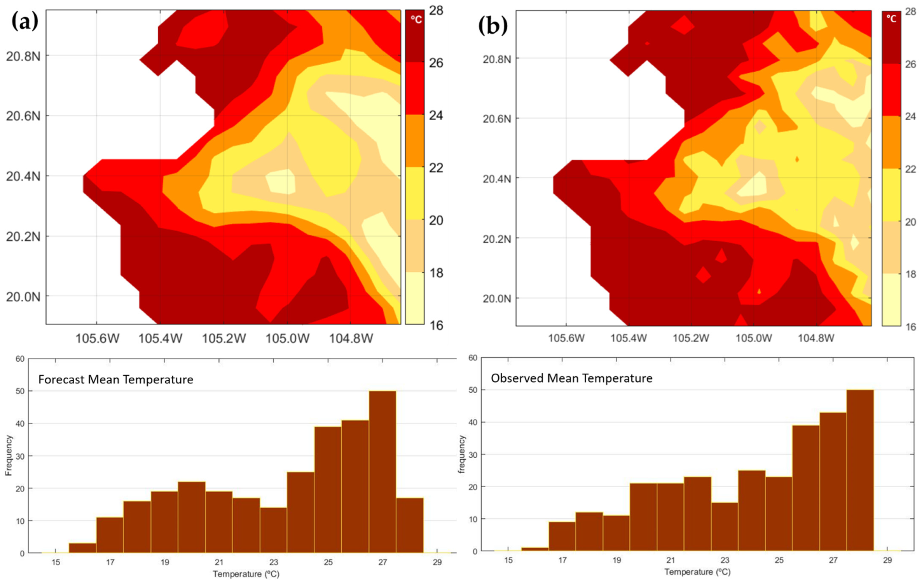
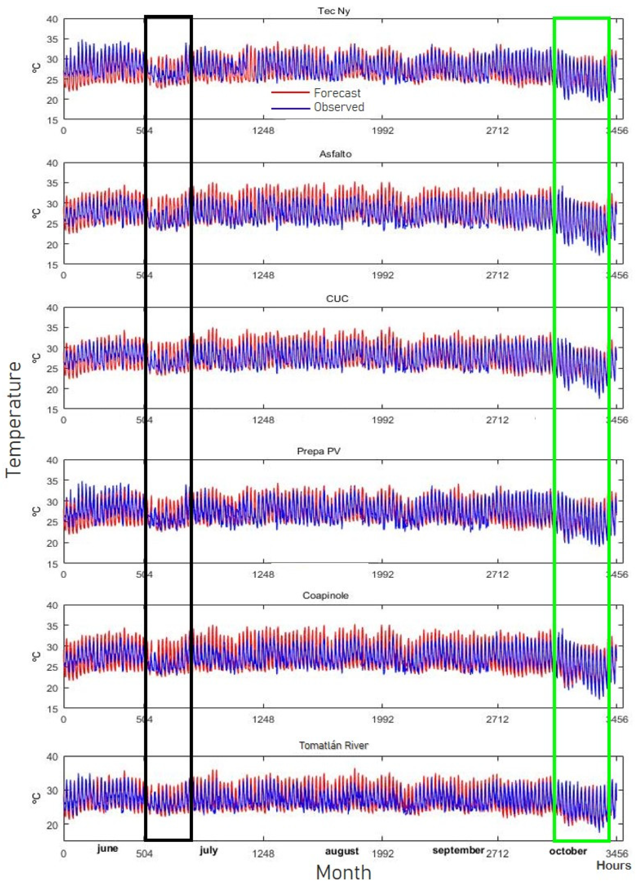
We can see in Figure 3 the time series of the forecasted and observed temperature corresponding to the six validation points, from June to October 2010. The WRF model forecasted temperature as expected, i.e., it reflected the variability of both diurnal and nocturnal temperatures (

Table 6. Results of the statistical analysis of forecasted and observed temperatures. The first column shows the six meteorological stations (see Figure 1), and the rest of the column shows the results of the statistical parameters. RMSE, MAE, BIAS, stdD-F, stdD-O are in °C, meanwhile [−1 ≤ r ≤ 1].

#	Automatic MeteoroLogical Stations	stdD-F	stdD-O	r	RMSE	MAE	BIAS
1	Tec Ny	2.96	2.59	0.82	1.75	1.43	−0.53
2	Asfalto	3.22	2.58	0.84	1.91	1.47	0.79
3	CUC	3.15	2.48	0.84	1.73	1.36	0.2
4	Prepa PV	2.87	2.56	0.82	1.6	1.22	0.15
5	Coapinole	2.89	2.36	0.84	1.57	1.24	−0.31
6	Tomatlán River	3.6	2.68	0.87	1.85	1.45	0.28
	Average	3.12	2.54	0.84	1.74	1.36	0.1

). The model was able to forecast significant thermal oscillations, such as the low temperatures that occurred late in October (Figure 3; green box). However, on 1 July 2010, Hurricane Alex made landfall in Tamaulipas, moving inland and downgrading over the following days to a tropical storm and depression, before reaching the edge of the western coast of Mexico. According to the Servicio Meteorológico Nacional (SMN, México City, Mexico, by its Spanish acronym), this tropical depression left a low-pressure zone that generated sudden changes in air flows, first from the north and northeast and then from the west and northwest of the country. These flows caused reduced temperatures in the first days of July (Figure 3; black box), and the model, which had forecasted normal flows, could not predict these unexpected interactions.

The validation points show a bias between the forecasted and observed temperatures that did not exceed $\pm 1 °\mathrm{C}$ (Table 6). This is minor, according to Jolliffe and Stephenson [22], since it represents only between 10% and 25% of the standard deviation of temperature, except at the Asfalto station, in which the BIAS is 0.79, representing 30.6% of stdD-O. Nevertheless, the standard deviations of the forecasts (stdD-F) are higher in all cases than the observed values, indicating that the model overestimated higher temperatures and underestimated low temperatures. The model projected higher temperatures at four stations (Asfalto, CUC, Prepa PV, and Tomatlán River) and less high temperatures in two stations (Tec Ny and Coapinole). There is, on average, a good correlation between the forecast and the observation $\left(\mathrm{r}=0.84\right)$ of the six validation points. The errors ($\mathrm{RMSE}$ and $\mathrm{MAE}$) show values lower than$2 °\mathrm{C}$, indicating that the forecast errors are small and that the forecast presents adequate accuracy. In comparison, other studies show similar trends. In a validation analysis for the temperature of a WRF model in a subtropical region in India, the $\mathrm{RMSE}$ was $2.55–4.26 °\mathrm{C}$ for the nine simulations of summer conducted at two stations; meanwhile, $\mathrm{r}$ was $0.94–0.97$, and the $\mathrm{BIAS}$ ranged from $-0.11$ to $-0.01 °\mathrm{C}$ [27]. Challa et al. [43] reported a graphical analysis of the sensitivity of atmospheric dispersion simulations, where the WRF underestimated daily temperatures. When evaluating temperature for an air quality analysis in the northeast of the Iberian Peninsula, errors were found in the 2 km domain, the $\mathrm{RMSE}$ was 1.$5–3.8 °\mathrm{C}$, and the $\mathrm{BIAS}$ ranged from $-3$ to $1 °\mathrm{C}$ [44]. In an analysis of the weather event of 2007 related to the flood in Tabasco, Mexico, the errors ($\mathrm{RMSE}$ and $\mathrm{MAE}$) in the two sampling points were $1.6$ and $4.5 °\mathrm{C}$, respectively, while the $\left(\mathrm{BIAS}\right)$ was $-4.1$ and $0.2 °\mathrm{C}$, and $\mathrm{r}$ was 0.97 and $0.96$, respectively, for the 24 h forecasts [25].

For the elaboration of the average observed temperature map, the equation used was $y=28.27-0.00506x$ with $r^2=0.937$ and $p=0.00$. The thermal gradient for every 1000 m of altitude was $-5.06 °\mathrm{C}$ on average during the five months of validation. In other studies, the results were similar. Gomez et al. [35], for the estimation of the average temperature in Tepehuanes, Durango, Mexico, obtained an $r^2=0.926$ on average for June to October, while Ninyerola et al. [34], for the climatological modeling of the air temperature in Catalonia, Spain, obtained an $r^2=0.848$ on average for the five months of validation with the corrected temperature maps.

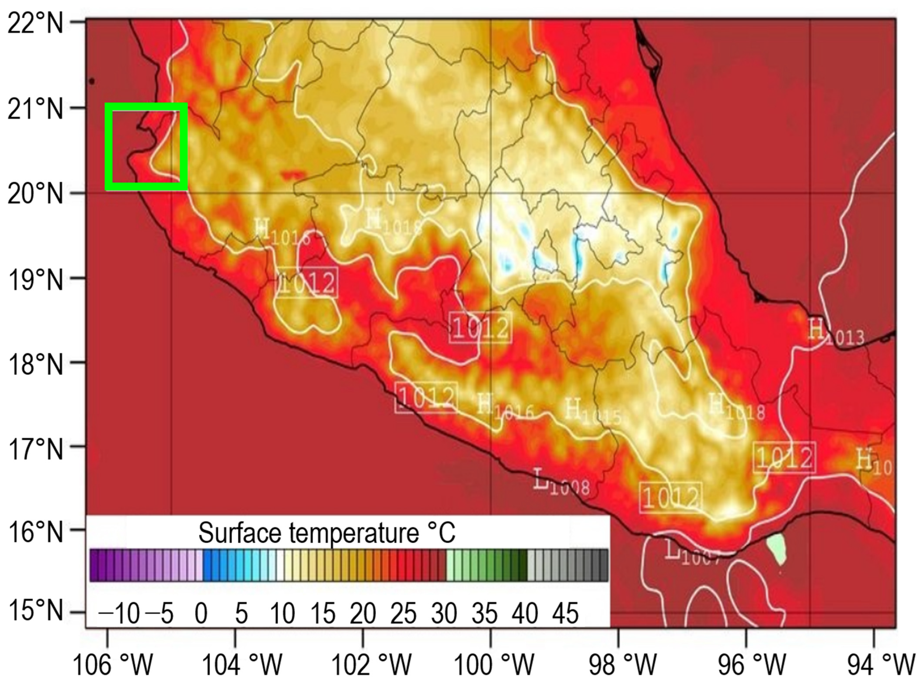
The spatial distribution of temperature predicted by the WRF model (Figure 4a) presented spatial thermal variability, similar to the observed temperature (Figure 4b). The model also accurately determined the warm zones, on the coast $\left(~28 °\mathrm{C}\right)$ and the temperate zones in the mountains $\left(16–18 °\mathrm{C}\right)$. We observed that the determining variable in the temperature in the study region is the type of topography. This corroborates what Magaña et al. [7], Ninyerola et al. [34] and Jorba et al. [44] reported. Spatially, the temperature followed a bi-modal distribution that was reasonably well projected by the model in its histogram when compared with the observed temperature (Figure 4).

The predicted spatial temperature distribution shows the same spread as the observed temperature, with a standard deviation value of $3.3 °\mathrm{C}$ (Figure 4). The $\mathrm{BIAS}$ was $-0.6 °\mathrm{C}$, indicating that the model slightly underestimated the observed temperature, with a correlation of $r=0.95$, while the $\mathrm{RMSE}$ was $1.23$, showing a slight reduction in forecast accuracy. As a background to these error results, a comparison can be made with the research of Flaounas et al. [26], where they performed a simulation of the West African monsoon in 2006 using the WRF, and the simulated temperatures in comparison with those observed for all of West Africa had a strong positive BIAS that reached $2 °\mathrm{C}$.

3.2. Precipitation Validation

For binary (yes/no) events, a “yes” event is defined for precipitation equal to or higher than a specified reference (in this study, it is 1 mm of accumulated rain in 24 h); otherwise, it is defined as a “no event”. The distribution of the observed days with rain and the days in which rain was not observed compared to those forecasted are shown in the next contingency table (

Table 7. Results of the indexes calculated for forecasted and observed precipitation accumulated during the period of 10 June–31 October 2010.

		Observed
		$\mathbf{Y}\mathbf{E}\mathbf{S}$	$\mathbf{N}\mathbf{O}$	Total
Forecast	$\mathrm{YES}$	92	32	124
	$\mathrm{NO}$	266	474	740
	Total	358	506	864

).

In contrast to the temperature analysis, the model showed poor performance in predicting the number of days with precipitation compared to what was observed. In contrast to the temperature analysis. The period of rain under assessment covered 144 days at six verification points, a total of 864 forecasts. From this total, the rain was observed on 358 days, which means that the model failed to predict 266 days, or 74.3% (Table 7 and

Table 8. The results of the calculated statistics are based on the results of the contingency table (Table 7). CI is the confidence interval for the $\mathrm{H}$, $\mathrm{FAR}$, and $\mathrm{PC}$ statistics. $\left[0\le \mathrm{H}\le 1\right]$, $\left[0\le \mathrm{FAR}\le 1\right]$, and $\left[0\le \mathrm{PC}\le 1\right]$.

Statistic	Value	CI	Comment
$\mathrm{H}$	0.257	0.214, 0.305	Probability of detection of days with rain.
$\mathrm{FAR}$	0.258	0.189, 0.341	Probability of false detection.
$\mathrm{PC}$	0.655	0.623, 0.686	The proportion of days with rain and without rain that was accurately forecasted.

). The correct proportion of days with rain forecasted $\left(\mathrm{H}\right)$ corresponds to 25.7%, with a $\mathrm{CI}$ of 95% (21.4%, 30.5%) (Table 8). The proportion of days with rain that represented false alarms $\left(\mathrm{FAR}\right)$ corresponds to 25.8%, with a $\mathrm{CI}$ of 95% (18.9%, 34.1%). Only PC shows a favorable performance with 65.5%, with a CI of 95% (62.3%, 68.6%). However, this index was influenced by the 474 days on which no rain occurred (Table 8).

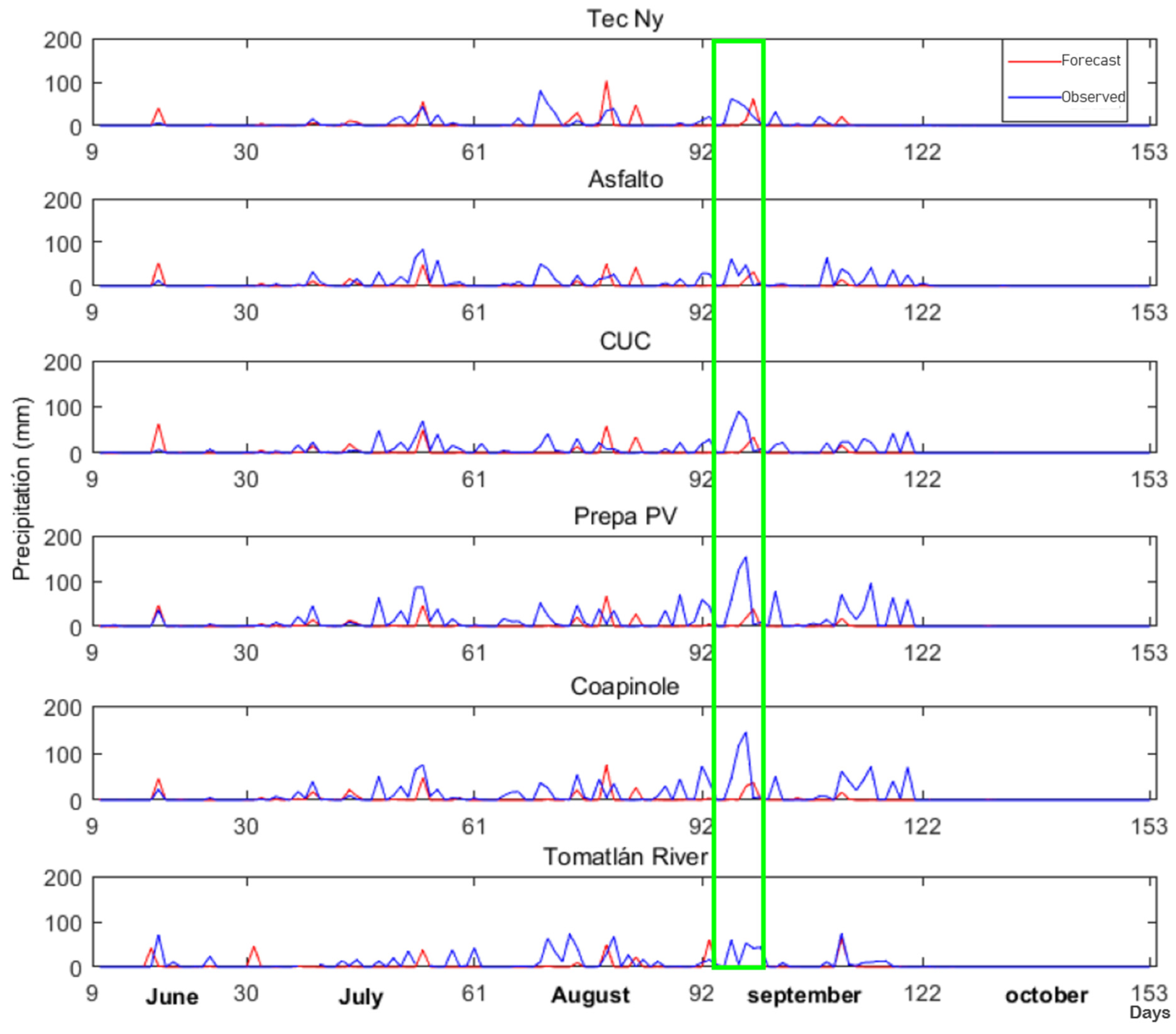
Severe events that occurred suddenly and could involve rainfall greater than 100 mm were not accurately forecasted (Figure 5). The temporal distribution of precipitation showed a very marked bias in the accumulated precipitation at the beginning of September (Figure 5, green rectangle).

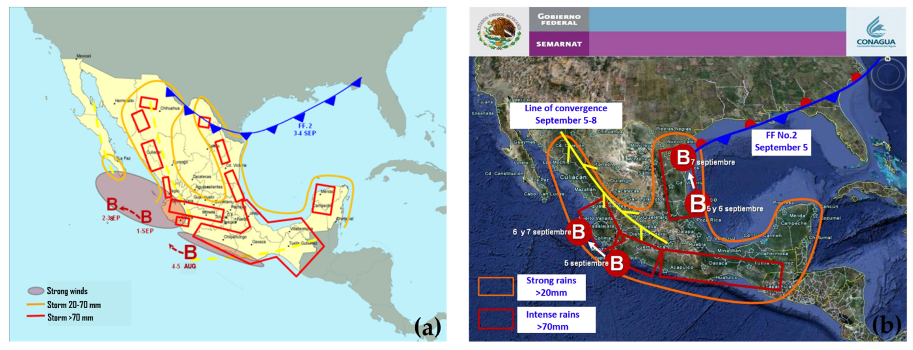
According to the SMN report, on 4 September 2010, a low-pressure convergence line formed over the western Sierra Madre and the Mesa Central (Figure 6). This generated the propagation of cloudy days with a high potential for rain and thunderstorms that caused precipitation exceeding 100 mm at the meteorological stations Prepa PV and Coapinole.

Table 9. Results of the statistical parameters of forecasted and observed precipitation accumulated during the period of 10 June–31 October 2010. The first column shows the six meteorological stations (see Figure 1), and the rest of the columns show the statistical results. RMSF, MAE, and BIAS are in millimeters, while $\left[-1\le r\le 1\right]$.

#	Meteorological Stations	$\mathit{r}$	$\mathbf{R}\mathbf{M}\mathbf{S}\mathbf{F}$	$\mathbf{M}\mathbf{A}\mathbf{E}$	$\mathbf{B}\mathbf{I}\mathbf{A}\mathbf{S}$
1	Tec Ny	0.27	15.32	6.19	−2.3
2	Asfalto	0.29	16.59	7.8	−5.44
3	CUC PV	0.22	16.99	7.93	−5.13
4	Prepa PV	0.24	27.28	12.38	−10.24
5	Coapinole	0.28	23.85	10.97	−8.31
6	Tomatlán River	0.23	17.78	7.88	−5.42
	Average	0.26	19.64	8.86	−6.14

shows the results of the statistical indices of the six validation points, suggesting the poor performance of the model, since the model underestimated the accumulated precipitation in 24 h periods, by between 2.3 mm and 10.24 mm. The correlation coefficients in the six sampling points were $<0.3$. The $\mathrm{RMSF}$ and $\mathrm{MAE}$ values in all cases were greater than 15 and 6 mm, respectively, showing a low performance in terms of forecast accuracy. In comparison, in an analysis for validating forecasts of accumulated rain to 24 h with WRF for all of Mexico, Corrales et al. [3] reported errors ($\mathrm{RMSF}$ and $\mathrm{MAE}$) of 6.25 mm and 2.26 mm, respectively, while the correlation was 0.35.

For the elaboration of the accumulated precipitation map during the study period, we used the equation $\mathrm{y}=2391.38-173.888{\mathrm{x}}^1-0.32496{\mathrm{x}}^2$, where ${\mathrm{r}}^2=0.389$ and $\mathrm{p}=0.11$. After the precipitation map was corrected, the ${\mathrm{r}}^2=0.478$ and $\mathrm{p}=0.00$. In contrast, Ninyerola et al. [34], for the climatological modeling of precipitation in Catalonia, Spain, obtained an ${\mathrm{r}}^2=0.818$ for June to October. First, we calculated multiple correlations including latitude and altitude; these variables were also used in the equation of Ninyerola et al. [34], but in our results ${\mathrm{r}}^2=0.235$ and $\mathrm{p}=0.30$; therefore, we used altitude and evaporation in our equation, and thus we obtained the highest value of ${\mathrm{r}}^2$.

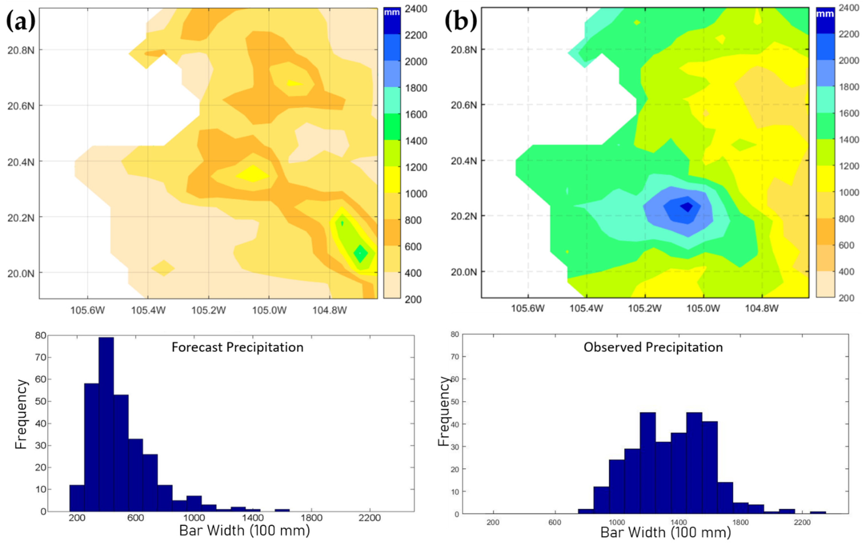
The spatial distribution of precipitation forecasted by the model was poor compared to that observed in the verification (Figure 7). Mean precipitation for the entire period (10 June–31 October 2010) was forecasted at 503 mm, but 1355 mm was observed. WRF underestimated the accumulated precipitation during the entire study period, with a $\mathrm{BIAS}$ of $-852$mm; meanwhile, the average degree of correspondence between individual pairs of predicted and observed values $\left(\mathrm{RMSE}\right)$ was $930$mm and produced the histograms shown in Figure 7. Despite the above, the model (Figure 7a) was able to predict areas of high precipitation (the Tuito Mountains, La Bufa Hill, and Cacoma Mountain) and of lower precipitation (the coastal zone and the Ameca River Valley), very similar to what was observed. The value of the $\mathrm{RMSF}$ index is very close to 2 ($\mathrm{RMSF}=1.96$), indicating that the WRF was able to predict where higher and lower precipitation occurred; however, it underestimated the accumulated precipitation for the entire period, with a $\mathrm{BIAS}$ of 813 mm (Table 9) and produced the histograms shown in Figure 7. Other researchers found similar results—for example, Flaounas et al. [26] found, in a simulation of the West African monsoon in 2006 using the WRF, that the precipitation pattern was generally modeled to an adequate level, although these authors acknowledged that convective rainfall is a constantly changing variable that is difficult to model. Casati [28], in his thesis for the evaluation of the NIMROD model for spatial rain forecasting in the United Kingdom, found values of $\mathrm{RMSE}$ and $\mathrm{MAE}$ that were $<3$, while the value of correlation was less than 0.4 in the eight case studies and the $\mathrm{RMSF}$ index was between 1.75 mm and 9.27 mm. Magaña et al. [7], in their MM5 model evaluation for rain forecasting in periods of 24 h for Mexico City, found large spatial differences in August during the period of 2008–2010. They reported that in the south and southwest of Mexico City, the rain was overestimated by approximately 50 mm, while in the western area where greater precipitation was observed, the model underestimated the precipitation by approximately 200 mm from a total of 300 mm and, on the east side of the city, the difference was approximately 50 mm.

Regarding short-term forecasting in the BB region, relatively little is known about the quality of predictions from models that are run on a national or regional scale. When high-resolution spatial forecasts are performed in cases where ground effects are important, the quality of the forecasted rainfall is limited by different spatial patterns [7]. Another limiting factor is working at a low resolution (50 km) to save computational resources, for example in the analysis of the African monsoon reported by Flaounas et al. [26]. In this context, Flores [29] pointed out that the differences between the predicted and observed variables are because the model simplifies and smoothes the surface processes by representing them in a grid of 18 km resolution. Meanwhile, Jorba et al. [44] found that the simulation with a high horizontal resolution (2 km grid) in the geographic area of Catalonia, Spain, can allow the analysis of the possible atmospheric circulation that occurs. In correspondence with the above and taking into account these limitations in the quality of the forecasts, we have evaluated the output results of the WRF at the working resolution (7 km).

4. Conclusions

The use of numerical models such as the WRF for weather forecasting has become a fundamental tool to support decision-making both at the government level and in society in general, and is also of great value for atmospheric research. Thus, in this research and based on the statistical results, we have concluded that the temperature forecasts of the WRF model for the BB region were acceptable concerning what was observed during the study period. Meanwhile, the precipitation forecasts were not consistent with what was observed, especially in severe weather events (hurricanes, electric storms), and due to the complex topography of the study area. A study involving the use of the model at the regional and local levels is recommended to increase its resolution and improve its performance in weather forecasting. The configuration, operation, and evaluation of these findings will be of interest not only for short-term meteorological purposes but also for decision making in daily activities.

References

1. Tapiador, F.; Navarro, A.; Levizzani, V.; García-Ortega, E.; Huffman, G.; Kidd, C.; Kucera, P.; Kummerow, C.; Masunaga, H.; Petersen, W.; et al. Global precipitation measurements for validating climate models. Atmos. Res. 2017, 197, 1–20. [Google Scholar] [CrossRef]
2. Prieto, R.; Avendaño, M.A.; Ramírez, L.G.M.; Eslava, H. Tormentas Severas. Serie Fascículos; Centro Nacional de Prevención de Desastres-Secretaría de Seguridad y Protección Ciudadana: Mexico City, Mexico, 2010; ISBN 9786077558088. [Google Scholar]
3. Corrales, A.; Narváez, M.P.; Ruíz, O.; Flores, H.; González, L.A.; González, M.A.; Maciel, L.H. Validación del pronóstico de lluvia acumulada mediante el modelo wrf para la república mexicana. In Semana Internacional de Agronomía; Vázquez Navarro, J.M., Puentes Gutiérrez, J., Martínez Ríos, J.J., López Calderón, M.J., de Jesús Vázquez Navarro, M., Camacho Rodríguez, S.Y., Santana Rodríguez, R., Eds.; Universidad Juárez del Estado de Durango: Durango, Mexico, 2014; p. 6. [Google Scholar]
4. Vega-Serratos, B.E.; Domínguez-Mora, R.; Posada-Vanegas, G. Evaluación estacional del riesgo por inundación en zonas agrícolas. Tecnol. y Cienc. del Agua 2018, 9, 92–127. [Google Scholar] [CrossRef]
5. Beguería, S.; Vicente-Serrano, S.M.; López-Moreno, J.I.; García-Ruiz, J.M. Annual and seasonal mapping of peak intensity, magnitude and duration of extreme precipitation events across a climatic gradient, northeast Spain. Int. J. Clim. 2009, 29, 1759–1779. [Google Scholar] [CrossRef] [Green Version]
6. Merz, B.; Kreibich, H.; Schwarze, R.; Thieken, A. Review article: Assessment of economic flood damage. Nat. Hazards Earth Syst. Sci. 2010, 10, 1697–1724. [Google Scholar] [CrossRef]
7. Magaña, V.; López, L.C.; Vázquez, G. El pronóstico de lluvias intensas para la Ciudad de México. Rev. Espec. en Cienc. Químico-Biológicas 2013, 16, 18–25. [Google Scholar] [CrossRef] [Green Version]
8. Valdés Verde, A.; Cruz Rodríguez, R.C.; Roque Rodríguez, A. Evaluación del pronóstico de viento del modelo Weather Research Forecast (WRF) en torres de prospección eólica. Rev. Cuba. De Meteorol. 2015, 21, 16–28. [Google Scholar]
9. Díaz, Y. Evaluación del Pronóstico Numérico del Tiempo a Corto Plazo Para Cuba Con el Modelo de Mesoescala MM5V3; Instituto Superior de Tecnologías y Ciencias Aplicadas: Havana, Cuba, 2010. [Google Scholar]
10. Gutierrez, J.M.; Cano, R.; Cofiño, A.S.; Sordo, C.M. Redes Probabilísticas y Neuronales en las Ciencias Atmosféricas; Miniesterio de Medio Ambiente: Madrid, Spain, 2004; ISBN 8483202816. [Google Scholar]
11. Sikder, S.; Hossain, F. Assessment of the weather research and forecasting model generalized parameterization schemes for advancement of precipitation forecasting in monsoon-driven river basins. J. Adv. Model. Earth Syst. 2016, 8, 1210–1228. [Google Scholar] [CrossRef] [Green Version]
12. Litta, A.J.; Ididcula, S.M.; Mohanty, U.C.; Prasad, S.K. Comparison of Thunderstorm Simulations from WRF-NMM and WRF-ARW Models over East Indian Region. Sci. World J. 2012, 2012, 1–20. [Google Scholar] [CrossRef] [Green Version]
13. Powers, J.G.; Klemp, J.B.; Skamarock, W.C.; Davis, C.A.; Dudhia, J.; Gill, D.O.; Coen, J.L.; Gochis, D.J.; Ahmadov, R.; Peckham, S.E.; et al. The Weather Research and Forecasting Model: Overview, System Efforts, and Future Directions. Bull. Am. Meteorol. Soc. 2017, 98, 1717–1737. [Google Scholar] [CrossRef]
14. Matsudo, C.; Salles, M.A.; García Skabar, Y. Verificación de los Pronósticos del Esquema Determinístico del Modelo WRF Para el Año 2020; Servicio Meteorológico Nacional Argentina: Buenos Aires, Argentina, 2021. [Google Scholar]
15. López, M.R.; Núñez-Cornú, F.J.; Plascencia, C.S. Study of Seismic Clusters at Bahía de Banderas Region, Mexico. Geofís. Int. 2013, 52, 59–72. [Google Scholar] [CrossRef] [Green Version]
16. Velázquez Ruiz, A.; Manuel Martínez, L.R.; Carrillo González, F.M. Caracterización climática para la región de Bahía de Banderas mediante el sistema de Köppen, modificado por García, y técnicas de sistemas de información geográfica. Investig. Geográf. 2012, 7–19. [Google Scholar] [CrossRef]
17. Cupul-Magaña, F.G. Bahía de Banderas: Un escaparate para la contemplación de las aves. Rev. Mex. 2001, 3, 45–58. [Google Scholar]
18. INEGI.CONTINUO DE ELEVACIONES MEXICANO (CEM). Available online: https://www.inegi.org.mx/app/geo2/elevacionesmex/index.jsp (accessed on 24 June 2021).
19. Paulhus, J.L.H.; Kohler, M.A. Interpolation of missing precipitation records. J. Frankl. Inst. 1952, 138, 129–133. [Google Scholar] [CrossRef] [Green Version]
20. Skamarock, W.C.; Klemp, J.B.; Dudhia, J.; Gill, D.O.; Barker, D.M.; Duda, M.G.; Huang, X.-Y.; Wang, W.; Powers, J.G. A Description of the Advanced Research WRF Version 3; University Corporation for Atmospheric Research: Boulder, CO, USA, 2008. [Google Scholar]
21. WWRP/WGNE Joint Working Group on Verification. Recommendations for the Verification and Intercomparison of QPFs from Operational NWP Models. 2004. Available online: https://www.cawcr.gov.au/projects/verification/WGNE/QPF_verif_recomm.pdf (accessed on 24 June 2022).
22. Jolliffe, I.T.; Stephenson, D.B. Forecast Verification: A Practitioner´s Guide in Atmospheric Science; John Wiley & Sons: West Sussex, UK, 2003; ISBN 0470864419. [Google Scholar]
23. Wilks, D.S. Statistical Methods in the Atmospheric Sciences, 2nd ed.; Wilks, D.S., Ed.; Academic Press: San Diego, CA, USA, 2006; Volume 100, ISBN 978-0-12-385022-5. [Google Scholar]
24. JWGFVR. Methods for Dichotomous (Yes/No) Forecasts. Available online: https://www.cawcr.gov.au/projects/verification/ (accessed on 24 June 2022).
25. López Méndez, J.V. Análisis del Evento Meteorológico del 2007 Relacionado con la Inundación de Tabasco. Master’s Thesis, Universidad Nacional Autónoma de México, Mexico City, Mexico, 2009. [Google Scholar]
26. Flaounas, E.; Bastin, S.; Janicot, S. Regional climate modelling of the 2006 West African monsoon: Sensitivity to convection and planetary boundary layer parameterisation using WRF. Clim. Dyn. 2011, 36, 1083–1105. [Google Scholar] [CrossRef]
27. Mohan, M.; Bhati, S. Analysis of WRF Model Performance over Subtropical Region of Delhi, India. Adv. Meteorol. 2011, 2011, 1–13. [Google Scholar] [CrossRef] [Green Version]
28. Casati, B.; Ross, G.; Stephenson, D.B. A new intensity-scale approach for the verification of spatial precipitation forecasts. Meteorol. Appl. 2004, 11, 141–154. [Google Scholar] [CrossRef] [Green Version]
29. Flores Rojas, J.E. Validación de Pronósticos de Temperatura y Precipitación con el modelo operacional de Mesoescala MM5 para la Costa Norte de Perú. In Compendio de Trabajos de Investigación Realizados Por Estudiantes Durante el Año 2003; Tavera, H., Ed.; Instituto Geofísico del Perú: Lima, Peru, 2004; p. 200. [Google Scholar]
30. World Meteorological Organization. Recommendations for the Verification and Intercomparison of QPFs and PQPFs from Operational NWP Models; World Meteorological Organization: Geneva, Switzerland, 2008; Volume 41. [Google Scholar]
31. Castro, L.M.; Gironás, J.; Fernández, B. Spatial estimation of daily precipitation in regions with complex relief and scarce data using terrain orientation. J. Hydrol. 2014, 517, 481–492. [Google Scholar] [CrossRef]
32. Daly, C.; Neilson, R.P.; Phillips, D.L. A Statistical-Topographic Model for Mapping Climatological Precipitation over Mountainous Terrain. J. Appl. Meteorol. Climatol. 1994, 33, 140–158. [Google Scholar] [CrossRef] [Green Version]
33. Agresti, A.; Coull, B.A. Approximate Is Better than “Exact” for Interval Estimation of Binomial Proportions. Am. Stat. 1998, 52, 119. [Google Scholar] [CrossRef]
34. Ninyerola, M.; Pons, X.; Roure, J.M. A methodological approach of climatological modelling of air temperature and precipitation through GIS techniques. Int. J. Clim. 2000, 20, 1823–1841. [Google Scholar] [CrossRef]
35. Gómez, J.D.; Etchevers, J.D.; Monterroso, A.I.; Gay, C.; Campo, J.; Martínez, M. Spatial estimation of mean temperature and precipitation in areas of scarce meteorological information. Atmósfera 2008, 21, 35–56. [Google Scholar]
36. Noori, M.J.; Hassan, H.H.; Mustafa, Y.T. Spatial Estimation of Rainfall Distribution and Its Classification in Duhok Governorate Using GIS. J. Water Resour. Prot. 2014, 6, 75–82. [Google Scholar] [CrossRef] [Green Version]
37. Price, D.T.; McKenney, D.W.; Nalder, I.A.; Hutchinson, M.F.; Kesteven, J.L. A comparison of two statistical methods for spatial interpolation of Canadian monthly mean climate data. Agric. For. Meteorol. 2000, 101, 81–94. [Google Scholar] [CrossRef]
38. Dobesch, H.; Dumolard, P.; Dyras, I. (Eds.) Spatial Interpolation for Climate Data: The Use of GIS in Climatology and Meteorology; ISTE Ltd.: London, UK, 2007; ISBN 978-1-905209-70-5. [Google Scholar]
39. Crochet, P.; Jóhannesson, T.; Jónsson, T.; Sigurðsson, O.; Björnsson, H.; Pálsson, F.; Barstad, I. Estimating the Spatial Distribution of Precipitation in Iceland Using a Linear Model of Orographic Precipitation. J. Hydrometeorol. 2007, 8, 1285–1306. [Google Scholar] [CrossRef]
40. Portalés, C.; Boronat, N.; Pardo-Pascual, J.E.; Balaguer-Beser, A. Seasonal precipitation interpolation at the Valencia region with multivariate methods using geographic and topographic information. Int. J. Clim. 2010, 30, 1547–1563. [Google Scholar] [CrossRef] [Green Version]
41. Golding, B.W. Nimrod: A system for generating automated very short range forecasts. Meteorol. Appl. 1998, 5, 1–16. [Google Scholar] [CrossRef]
42. Loikith, P.C.; Lintner, B.R.; Sweeney, A. Characterizing Large-Scale Meteorological Patterns and Associated Temperature and Precipitation Extremes over the Northwestern United States Using Self-Organizing Maps. J. Clim. 2017, 30, 2829–2847. [Google Scholar] [CrossRef]
43. Challa, V.S.; Indrcanti, J.; Baham, J.M.; Patrick, C.; Rabarison, M.; Young, J.H.; Hughes, R.; Swanier, S.J.; Hardy, M.G.; Yerramilli, A. Sensitivity of atmospheric dispersion simulations by HYSPLIT to the meteorological predictions from a meso-scale model. Environ. Fluid Mech. 2008, 8, 367–387. [Google Scholar] [CrossRef]
44. Jorba, O.; Jiménez, P.; Baldasano, J.M. Simulación anual con elevada resolución espacial para aplicaciones de la calidad del aire. In XXIX Jornadas Científicas de la Asociación Meteorológica Española; Asociación Meteorológica Española: Pamplona, Spain, 2006. [Google Scholar]
Figure 2. Central area of Mexico that shows the nesting of WRF model used in the Centro de Ciencias de la Atmósfera at UNAM. The green box indicated the validation area (BB region). This image corresponds to the 06:00 UTC forecast (1 September 2010).
Atmosphere 13 01220 g002
Figure 3. Forecasted (red) and observed (blue) temperature time series for each of the meteorological stations, per hour, from 00:00 h UTC on 10 June to 24:00 h UTC on 31 October 2010. The black rectangle shows low temperatures in early July due to Hurricane Alex. The green rectangle shows the low temperatures that occurred at the end of October.
Atmosphere 13 01220 g003
Figure 4. Forecasted and observed mean temperature maps with their respective histograms (10 June–31 October 2010). (a) Distribution of forecast mean temperatures; (b) distribution of mean temperatures observed.
Atmosphere 13 01220 g004
Figure 5. Forecasted (red) and observed (blue) precipitation time series for each of the meteorological stations, per day, from 00:00 h UTC on June 10th to 24:00 h UTC on 31 October 2010. The green rectangle corresponds to an event that occurred between 4 and 6 September 2010.
Atmosphere 13 01220 g005
Figure 6. Maps of the weather forecast generated by the Servicio Meteorológico Nacional (SMN) and Comisión Nacional del Agua (CONAGUA) for Mexico from 1 to 8 September 2010. The capital letter B shows the areas of low pressure on the Mexican Pacific coast and in the Gulf of Mexico. The solid and discontinuous yellow lines show the lines of convergence, both in (a,b). In (a), the line with blue triangles indicates a cold front in northern Mexico, and (b) indicates a stationary front. Images were obtained from the Weather Reports provided by the SMN and Conagua.
Atmosphere 13 01220 g006
Figure 7. Distribution of the accumulated forecasted and observed precipitation with the respective histograms (10 June–31 October 2010). (a) Distribution of accumulated forecast precipitation; (b) distribution of accumulated observed precipitation.
Atmosphere 13 01220 g007