Characteristics of Resuspended Road Dust with Traffic and Atmospheric Environment in South Korea

Abstract

Characterizing the influencing factors of resuspended dust on paved roads according to the atmospheric environment and traffic conditions is important to provide a basis for road atmospheric pollution control measures suitable for various road environments in the future. This study attempts to identify factors in the concentration of resuspended dust according to the level of road dust loading and PM₁₀ emission characteristics according to atmospheric weather environment and traffic conditions using real-time vehicle-based resuspended PM₁₀ concentration measuring equipment. This study mainly focuses on the following main topics: (1) the increased level of resuspended dust according to vehicle speed and silt loading (sL) level; (2) difference between atmospheric pollution at adjacent monitoring station concentration and background concentration levels on roads due to atmospheric weather changes; (3) the correlation between traffic and weather factors with resuspended dust levels; (4) the evaluation of resuspended dust levels by road section. Based on the results, the necessity of research to more appropriately set the focus of analysis in order to characterize the resuspended dust according to changes in the traffic and weather environment in urban areas is presented.

1. Introduction

Particulate matter (PM) with diameters of less than 10 μm can cause various damages to the human body, such as respiratory failure and mental illness [1]. Additionally, their concentrations are often elevated close to roadways [2]. PM is caused through the contribution of effective road management, so the degree of contamination must be determined by including a quantitative analysis of contamination to determine if it is important enough to implement control measures. Road dust (RD) is generated and diffused by traffic, and it is one of the main causes of road pollution in cities. It is categorized as an exhaust emission (EE). For example, exhaust emissions include emissions from internal combustion locomotives and automobiles. In addition, nonexhaust emissions (NEEs) are generated by vehicles driving on roads [3]. In recent decades, it has been known that direct emissions from tailpipes have been reduced significantly due to the strengthening of exhaust emission standards applied to vehicle air masses and the extensive implementation of catalytic converters and diesel particulate filters [4]. However, it has been suggested that the main cause of failure to derive an effective reduction in PM₁₀ in large cities is the undervaluation and neglect of NEEs, which consist of road dust, tire wear, road wear, and brake wear particles caused by tire–road friction [5]. It also emphasizes that emissions from road traffic contribute to PM concentrations to at least the same extent as exhaust emissions [3,4,6,7,8].

According to the 2017 Clean Air Policy Support System (CAPSS), which provides the extent of the emissions of air pollutants in the Republic of Korea, resuspended dust from roadways makes up 45% of the total concentration of dust. Therefore, as an alternative to the main management of suspended dust in urban components, road cleaning programs by local governments are used extensively. It is important to properly design and implement road cleaning in consideration of road dust characteristics and climate and weather characteristics because of the economic uncertainty caused by short-term effects without considering cleaning methods, regional characteristics, and weather characteristics [9]. However, the reason for the difficulty of establishing the characteristics of dust that is resuspended from roadways is that the study to estimate the concentration of resuspended dust through the establishment of related processes and modeling is still at the basic level [10,11]. Furthermore, due to the large fluidity characteristics of very small substances, i.e., smaller than PM₁₀, research to determine the chemical profile of dust on roads composed of meteorological environments, transportation activities, and construction requires significant resources and time.

In this study, the concentration of silt loading (sL), resuspended dust of PM₁₀, and floating dust PM₁₀ on paved roads separated by space was measured, and the results were used to analyze the concentration of resuspended dust on paved roads in urban areas. The PM₁₀ concentration measured during operation quantified the characteristics of PM₁₀ based on the analysis of PM₁₀ information of the air pollution monitoring station, weather information of the competent meteorological station, and traffic information measured through the use of a vehicle detection system (VDS). Previous studies have shown the physical and chemical properties of fine dust on Mars by testing re-entrained aerosol kinetic emissions from road (TRAKER) equipment for real-time monitoring. The equipment has the advantage of being able to immediately investigate dust emissions on many roads with long sections [12,13,14]. This clearly states that the fine dust concentration measured by the system can be used to quantify the relationship between major factors for increasing road particle emissions by utilizing repeated measurements of resuspended dust to supplement the realistic limitations of AP-42. Various studies in these fields were mainly for identifying the emission characteristics or chemical profiles of the resuspended dust from roads [15,16,17,18,19,20,21] and a few studies considered the spatial and time variations in the major parameters [22].

The main purpose of this study was to provide an experimental basis for future road environmental changes by analyzing and characterizing the main emission characteristics of the PM₁₀ concentrations measured on paved roads that are caused by sL, air pollution, meteorological variables, and traffic conditions. In this study, we focused on this and tried to establish a process to secure data reliability by constructing a resuspended PM₁₀ measurements system and by observing the concentration of resuspended dust in separate sections of a road, i.e., sections less than 500 m in length.

2. Materials and Methods

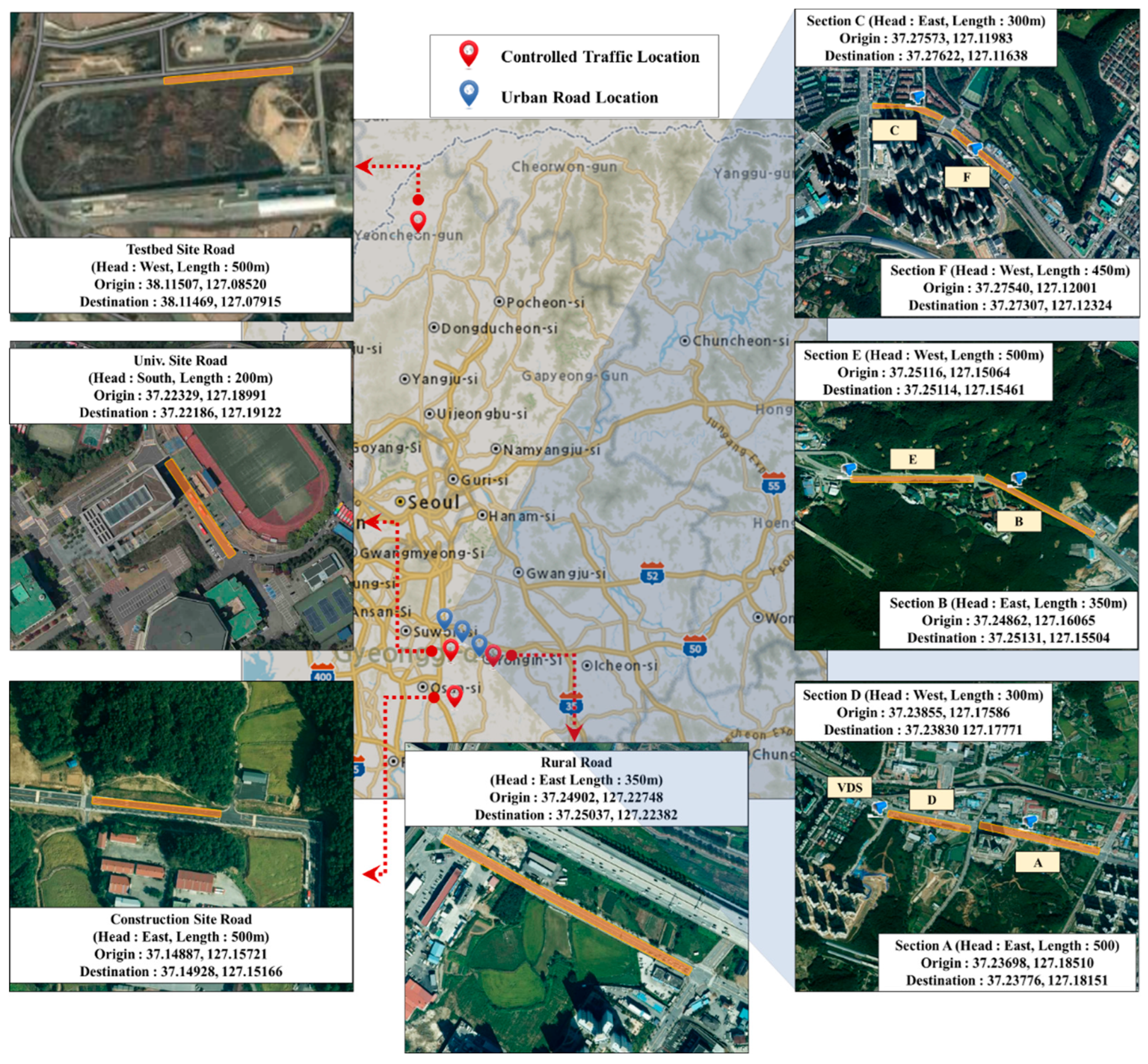
2.1. Study Area

To present a reasonable classification of the characteristics of PM₁₀ emissions on roads, locations were selected that were representative of vehicle-operating conditions and environmental characteristics. Measurements were held during periods without traffic impact observed in four sections from September to October 2021. During the measurement period, there were no weather events such as rainfall (0.01 inches of rain) that could have had a major effect on the fine dust concentration [23,24]. In addition, another measurement was determined on the concentration of resuspended dust on paved roads where traffic operated (Figure 1). Additionally, background PM₁₀ data (Bg) and weather variables and traffic condition data were collected through the urban atmosphere and traffic monitoring system at the same time. The traffic data were collected in six directions in three adjacent areas where traffic volume VDS was installed (

Table 1. Road conditions of the measurement section and distance from the observation.

Category	Site	Length (m)	Road Width/Condition	Distance of the Observation
				City Bg PM10	Meteorological Variables
Controlled Traffic	Testbed	500	One-lane road	With a radius of 2.5 km	With a radius of 24 km
	Construction Site	500	Two-lane road	With a radius of 3.5 km	With a radius of 20 km
	Univ.	200	One-lane road	With a radius of 1.6 km	With a radius of 14.5 km
	Rural	350	Two-lane road	With a radius of 2.8 km	With a radius of 17.5 km
Operating road	A	500	Four-lane road/ 905 (Veh/time/day)	With a radius of 8 km	With a radius of 14.5 km
	B	350	Three-lane road/ 633 (Veh/time/day)	With a radius of 5 km	With a radius of 11.5 km
	C	300	Four-lane road/ 1006 (Veh/time/day)	With a radius of 1 km	With a radius of 8.2 km
	D	300	Four-lane road/ 850 (Veh/time/day)	With a radius of 8 km	With a radius of 13.2 km
	E	500	Three-lane road/ 431 (Veh/time/day)	With a radius of 5 km	With a radius of 11 km
	F	450	Four-lane road/ 697 (Veh/time/day)	With a radius of 1 km	With a radius of 8.5 km

).

2.2. Resuspended PM₁₀ Measuring System

Road dust generated by vehicles driving on urban roads is known to have the greatest impact on the concentration of PM depending on the size of the sL collected on the surface of the road and the load and speed of the vehicles being driven on the road [11,14]. However, the method of measuring fine dust by performing and comparing direct dust collection activities through human activities on roads has safety and efficiency problems, and there are practical limitations in observing real-time concentrations. Mobile resuspended dust measurement systems were developed and implemented in the early 2000s. Scamper, TRAKER, and others generally use a method to calculate the difference between background concentration and tire measurements [12].

By establishing a real-time mobile dust measurement system based on the Desert Research Institute (DRI)’s TRAKER method, the temporal and spatial distribution characteristics of the resuspended dust on urban pavement can be checked and the impact of road dust sources can be confirmed by traffic and environmental factors [25].

The resuspended PM₁₀ measurement system (Figure 2) used an optical sensor that inhaled PM every second to determine the PM₁₀ concentration on the road through the front (mounted on the hood) inlet of the vehicle and the rear (right front wheel) inlet of the tire [25]. In quantifying the optical and physical characteristics of resuspended dust, the measurement of real-time dust concentration used scattered light to measure the weight of dust passing through. The measurement method clearly states that the concentration of resuspended dust can be measured [26].

To summarize, the equipment contains six main components, i.e.,:

• Vehicle specifications: 2016 SUV Sportage 2.02 WD, Tire Model 225/60R17.
• PM₁₀ Sensor: The 8530 Dust-Trak Optical PM Sensor Model (TSI Company, Shoreview, MN, USA) with PM₁₀ inlet is a portable device that can measure the concentrations of various sizes of dust particles in real time, such as PM₁₀ and PM_2.5.
• Inlet: The right tire line inlet is 175 mm above the ground and 50 mm behind the tire. The PM₁₀ concentration (C_i) obtained from the back of the tire during movement indicates that the air velocity measured along the center of the tire was not affected significantly by the surrounding wind direction at a distance less than 100 mm from the tire [27].
• Uniform Velocity Flow Sampling Inhalation: A vacuum pump is controlled by a customized suction port to adjust the pressure of the suction port appropriately, thereby producing a pressure-free suction port, so the air flow that is being sampled has the same fluid flow as the surrounding air flow.
• Data Collection System: Laptop computers were used to collect and transmit Dust-Trak data at one-second intervals.
• Monitoring Camera: A camera capable of monitoring the inside and outside of the vehicle can be installed to visually cross-verify the measurement data in the driving section and monitor the speed observed on the vehicle’s speedometer.

2.3. AP-42 Silt Loading Collection

In order to collect fine dust on the surface of a paved road, a section of the road was sampled using an 800 W vacuum cleaner, 3 m² frame of silt loading sampling, a fine dust brush, and a 3 kW gasoline generator [23].

Dust was immediately collected in the chamber, and it was eventually collected from the quartz fiber filters. At least three samples with different aerodynamic diameters were taken from a surface area of 3 m² for field sampling to reduce errors [28]. The samples were weighed using 200 mesh, standard Taylor screens, and a sieve filter machine.

2.4. Collecting City PM₁₀, Meteorological Variables, and Traffic Data

The data were collected as external impact indicators to analyze the effects of changes in the meteorological variables and traffic conditions on the PM₁₀ concentration levels observed through the resuspended PM₁₀ measurements system [29,30]. The collected elements were PM₁₀, the temperature of the ground (Gr temp), relative humidity (RH), wind speed (WS), sea level pressure, visibility, and time of after rainfall (rainfall time). The traffic data observed with adjacent VDS devices were divided into sections during the measurement period.

3. Results and Discussion

3.1. Verification of the Real-Time Measuring System

As a method of quantifying the concentration of road dust by sections using a mobile, real-time, PM₁₀ monitoring system, the concentration data measured with the inlet built into the front bumper of the vehicle were set to the background PM₁₀ concentration (C_Bg). This value was obtained by subtracting the background concentration from the resuspended PM₁₀ concentration (C_i) measured using the dust resuspended on the road along with the background concentration on the road through friction between the tires and the surface of the road. This value was quantified [31]. C_res was calculated according to the following equation:

$${\mathrm{C}}_{\mathrm{res}}=\frac{1}{\mathrm{n}}·{\displaystyle \sum }_{\mathrm{i}=1}^{\mathrm{n}}{\mathrm{C}}_{\mathrm{i}}-{\mathrm{C}}_{\mathrm{Bg}}$$

(1)

where C_res is the concentration of resuspended dust from the road surface (μg/m³), C_i is the PM₁₀ concentration measured in inches on the back of the tire resuspended dust concentration (μg/m³), C_Bg is the PM₁₀ concentration measured at the front bumper inlet of the vehicle background concentration (μg/m³).

Monitoring was performed to analyze the change in the concentration of resuspended dust due to sL in the space and time, where the concentration measured during the interval transit time varied by the inlet. The large changes meant that the C_Bg measurement was more than 100 μg/m³ within a short measurement period, and C_i measured on the back of the tire was more than 1000 μg/m³. Unlike the sL effects, this was proven to be an effect of the road dust as well as the external effects, such as the exhaust gas of other vehicles and the addition and deceleration of vehicles. Considering the average PM₁₀ concentration was 50 μg/m³ and the 24 h average PM₁₀ concentration was 100 μg/m³ level, it was excluded as an outlier. This was based on previous studies that indicated that the change in the C_Bg level when the vehicle was not moving was not affected significantly by the exhaust of other vehicles, and the concentration of C_i measured on the back of the tire could be used as the concentration of resuspended dust [13].

The process of verifying that the monitoring system can perform data collection functions for quantifying the concentration of road dust was conducted under three experimental conditions that could determine whether the measured concentration of the dust was significant when the vehicle moved.

(1)

We ensured that the measured concentration did not vary significantly when the vehicle stopped, and tried to calculate the range of the measured speed by comparing the concentration measured by increasing the speed as it passed the section at a constant speed.

(2)

If a certain measurement speed was maintained, the average C_res concentration measured in a short section and the amount of dust accumulated on the surface of the road and the concentration of the resuspended dust due to vehicle travel were quantified by the sL collected at three different locations in the section.

(3)

The correlation was analyzed by comparing the concentration of C_res measured by the size of sL in different sections (regions) selected by classification according to the major causes of the inflow of the expected material.

In the absence of peripheral vehicles, the monitoring system maintained a constant stop period and a constant speed, and the C_Bg value measured during the driving period maintained a constant slight change of approximately 2 to 6 μg/m³ per second. When the sL level collected in the section was 0.43 g/m² for the mean and 0.16 g/m² for the SD, the concentration was measured by maintaining 30, 40, 50, and 60 km/h, respectively, to analyze the effect on changes in the C_res concentration as the speed increased during the section (

Table 2. C_res concentration mean and standard deviation value measured with car speed in testbed.

Car Speed (km/h)	Cres Mean (μg/m3)	Cres SD (μg/m3)
30	23.0	3.4
40	54.6	14.8
50	69.1	18.9
60	93.0	21.3

).

The expression for increasing C_res concentration by velocity was the same as in Equation (2) (Figure 3).

$$\mathrm{y}=7.2971{\mathrm{e}}^{0.0442\mathrm{x}}$$

(2)

3.2. sL and Resuspended Dust on Paved Roads with Different Inflow Conditions

The results of measuring the concentration of sL and resuspended dust in sections with different fine dust generation and management environments while maintaining a speed of 50 km/h, which usually is used as the speed limit on roads operating in the center of the city, are presented in

Table 3. Concentration of sL, resuspended PM₁₀ on paved roads without any traffic.

Section		sL 1 (g/m2)	sL 2 (g/m2)	sL 3 (g/m2)	Mean sL (g/m2)	Bg PM10 (μg/m3)	Mean Ci PM10 (μg/m3)	Mean CBg PM10 (μg/m3)	Mean Cres PM10 (μg/m3)
Construction Site Road		0.115	0.089	0.074	0.093	30	242	17	225
Testbed Road	Day 1	0.024	0.038	0.039	0.034	13	51	4	47
	Day 2	0.043	0.044	0.042	0.043	18	77	4	73
	Day 3	0.062	0.068	0.063	0.064	26	93	11	81
	Day 4	0.069	0.08	0.075	0.075	21	91	10	81
Univ. Site Road	Day 1	0.002	0.002	0.002	0.002	10	40	11	29
	Day 2	0.003	0.003	0.003	0.003	16	41	17	24
	Day 3	0.005	0.005	0.007	0.006	23	50	22	28
	Day 4	0.009	0.01	0.008	0.009	36	58	37	21
Rural Road		0.007	0.006	0.003	0.005	58	77	66	11

and Figure 4. The sL collected at the entrance and exit of the construction vehicle next to the cement plant, where the traffic of medium-sized vehicles mainly occurred, was the highest at 0.093 g/m², and the concentration of resuspended dust was observed to be 225 μg/m³. For four consecutive days on the controlled testbed and low-traffic, university roads, the sL levels measured at the same time were found to continue to increase in deposition in the absence of specific events for rainfall, and the weather conditions observed were at a 11 μg/m³ C_res concentration (Table 3). As an influencing factor of resuspended dust generated on paved roads, it is known that the concentration level deposited on the section varies greatly depending on the heavy vehicle configuration and characteristics of traffic [32]. It has been shown that the resuspended dust from the road due to vehicle travel can be deposited, removed, moved into the air [23], or affected by weather conditions, geometric conditions, building geometry, etc. [29,33,34], or by regular road cleaning [9].

An analysis of the correlation between the C_res concentration and the collected sL measured when no ambient traffic occurred during the measurement and the space maintained was constant at 50 km/h speed on other roads showed a strong correlation, i.e., R² = 0.7586 (Figure 4). Depending on the increase in the sL level, the amount of C_res increases depended on the site being measured, which could vary depending on the source of the dust, but roughly represented a pattern in which the amount of resuspended dust along with the sL increased with the size of the sL.

3.3. Relationship between Section Background Concentration of Dust and Its Resuspended PM₁₀

Due to the relationship between C_Bg measured through the monitoring system and dust C_i resuspended due to driving, the impact of the sL size varied from site to site (Figure 5). If the observed concentration level was closer to the Y-axis, the tendency to increase the concentration of C_i compared to C_Bg was stronger, and the size of sL was less than 0.002 to 0.009 g/m² compared to 0.034 to 0.093 g/m², and the inclination of the C_Bg and C_i concentrations were closer to one. When the size of the sL gradually became higher than 0.034 g/m², it was observed that the concentration level of C_i increased linearly to show a difference of more than 47 to 225 μg/m³. In the 0.002 to 0.009 g/m² range, the difference of the C_i level of C_Bg was 11 to 29 μg/m³.

Such a level of sL below 0.01 g/m² was a level that could be collected on roads where traffic was continuous, such as general highways and highways where particulate matter was not special [35] and low resuspended dust was observed. C_Bg measured in a surrounding vehicle-free environment was found to increase with the level of air pollution (Bg) measured at adjacent stations at each measurement site, but the correlations were analyzed and found to have a strong correlation of R² = 0.8484 (Figure 6).

The measured C_Bg was 4 to 14 μg/m³, in Bg 10 to 20 μg/m³, 10 to 22 μg/m³, in Bg 20 to 30 μg/m³, 17 to 37 μg/m³, in Bg 30 to 40 μg/m³, and 50 to 60 μg/m³ in Bg 50 to 60 μg/m³. However, the increase may have varied depending on the spatial difference between the observed sections. This level was considered to be a significant result when comparing the report [36,37] that the mortality rates of all diseases, cardiopulmonary disease, and lung cancer increased significantly by 4%, 6%, and 8%, respectively, for every 10 μg/m³ increase in the concentration of particulate matter.

The relationship between Bg and C_Bg, measured during the running of the monitoring system on urban roads, was divided into two main patterns, i.e., (1) the yellow dust storm effect and (2) the no yellow dust storm effect. The yellow dust storm effect is a kind of dust fog, which is a phenomenon in which a large amount of yellow dust, which is called the continental yellow dust, drifts over a given area [38], indicating that the level of Bg and C_Bg measured at adjacent stations can vary greatly. The correlation between Bg and C_Bg measured on roads during traffic operation was relatively low compared to that of Bg and C_Bg measured on roads with limited traffic, and R² = 0.4697 was shown when the yellow dust phenomenon was excluded (Figure 7). It was found that differences in C_Bg also existed between sections in the same Bg and weather conditions observed by time zones at adjacent measuring stations. The difference was 20.45 μg/m³, with different levels of C_Bg on roads where the main sources of fine dust and inflow were judged to be similar. In addition, the occurrence of yellow dust was characterized by the opposite characteristics of the correlation R² = 0.1033 as the Bg level of the adjacent station became very high. The Regional Bg could be expected to have a quantitative impact on the overall pollution on roads, but when yellow dust occurred, the difference between C_Bg and Bg on roads could cause different concentration levels of C_res in the process of the continuous floating of road resuspended dust.

The correlation between C_Bg and C_i concentrations measured on roads during traffic operation showed a strong correlation of R² = 9253 without the influence of yellow dust, a weak correlation of R² = 0.4256 with yellow dust, and a correlation of R² = 0.8031 in respect to the overall concentration (Figure 8). The average concentration at which C_i was derived was 226 μg/m³, and the C_i concentration measured at the rear of the tire was the highest compared to C_Bg.

3.4. Analysis of PM₁₀ Concentration Characteristics of Resuspended Dust by Influencing Factors

For the correlation analysis between the concentration of resuspended dust measured on the road, atmosphere, meteorological variables, and traffic factors, dust measured data were collected (excluding yellow dust days data from the entire data) in six sections.

To analyze the effects of the average C_res concentration observed by road section on atmospheric and meteorological environments and traffic conditions, the C_res data samples were divided into five grades within the statistical analysis. (Lower quartile (25th): 7.7 μg/m³; median: 12.7 μg/m³; upper quartile (75th): 15.6 μg/m³; high C_res (sL level: over 0.009 g/m²): 29 μg/m³ were used.)

-

Low-level type: under 7.7 μg/m³.

-

Low- to middle-level type: 7.7 to 12.7 μg/m³.

-

Middle- to high-level type: 12.7 to 15.6 μg/m³.

-

High-level type: 15.6 to 29 μg/m³.

-

Bad-level type: over 29 μg/m³ and the number of measurements by C_res grade was the same as Figure 9.

Among them, the results of C_res measured as the bad level by section were observed in a wide range of Bg up to 15 to 113 μg/m³ (

Table 4. Comparison of observed C_res bad level concentrations by section and Bg concentration of the same time zone.

Section	Cres (μg/m3)	Bg (μg/m3)
A	33.1	103
	34.4	39
	47.6	55
B	31.4	15
	33.5	55
	36.7	46
	46.7	113
	69.4	104
C	56.7	58
D	32.6	55
E	29.5	58

). In different measured sections, C_res with the bad level was observed even at 15 μg/m³ in the level of concentration of Bg, and did not increase linearly. It is known that the Bg concentration and weather effects have a major influence on road atmosphere pollution, but it is difficult to represent them thoroughly, and it can be expected that external factors that are applied differently for each section are measured in the same time.

Since PM₁₀ on roads is known to be generated and diffused through various traffic elements, including traffic volume, traffic speed, road environment, and virtual elements [33], it is important to quantify the effect on the PM₁₀ concentration by reflecting the traffic characteristics of each section. The order of average C_res concentration and traffic by liver level was Location 2—Section B (18.0 μg/m³, 296 veh/time/lane) > Location 1—Section A (17.1 μg/m³, 324 veh/time/lane) > Location 3—Section C (12.7 μg/m³, 341 veh/time/lane) > Location 1—Section D (10.0 μg/m³, 318 veh/time/lane) > Location 2—Section E (9.4 μg/m³, 212 veh/time/lane) > Location 3—Section F (8.5 μg/m³, 245 veh/time/lane) (Figure 10).

C_i and C_Bg showed a relatively high consistent tendency when traffic was high by location, and C_res results when traveling in the eastern direction were higher than C_res when traveling in the western direction, but the C_res concentration did not appear in order depending on the traffic difference. In order to confirm the distribution of the lane traffic volume data sample, the lower quartile (25th) value or less were classified into lane traffic low level, the lower quartile (25th) value to median (50th) value were divided into lane traffic low to middle level, the median(50th) value to upper quartile (75th) value were divided into middle to high level, and the upper quartile (75th) value or higher value was divided into high level type (Figure 11).

Figure 12 shows the graph of the level type and road pollution levels C_i and C_Bg of lane traffic generated for each section. Relatively high C_res values were observed in sections with a relatively high frequency of occurrence of high-level lane traffic by location, and the results were as follows: Location 1—Section A (11 times, C_res: 17.1 μg/m³) vs. Section D (7 times, C_res: 10 μg/m³); Location 2—Section B (5 times, C_res: 18 μg/m³) vs. Section E (1 time, C_res: 9.4 μg/m³); Location 3—Section C (16 times, C_res: 12.8 μg/m³) vs. Section F (0 time, C_res: 8.5 μg/m³).

In addition, the lowest average C_Bg (47.5 μg/m³) and average C_i (56.9 μg/m³) concentrations were measured in Section E, where low-level lane traffic appeared 22 times.

3.5. Characteristics of C_i, C_Bg Resuspended Dust by Lane Traffic Level by Measurement Section through Statistical Probability Comparison

As

Table 5. Bg, C_Bg, C_i by interval and correlation analysis of major factors.

Independent		Correlation R-Value
		Ci	Bg	Lane Traffic	Gr Temp.	RH	WS	Sea Level Pressure	Visibility	Rainfall Time
Bg		0.66		0.04	−0.12	−0.14	−0.13	0.19	−0.35	0.41
Section A	CBg	0.95	0.62	−0.21	−0.24	0.36	−0.30	0.35	−0.60	0.44
	Ci		0.71	−0.14	−0.12	0.24	−0.27	0.25	−0.52	0.34
Section B	CBg	0.93	0.67	0.05	−0.28	0.29	−0.29	0.47	−0.59	0.48
	Ci		0.77	0.00	−0.11	0.18	−0.21	0.35	−0.46	0.43
Section C	CBg	0.96	0.70	−0.09	−0.29	0.16	−0.32	0.38	−0.50	0.44
	Ci		0.74	−0.17	−0.27	0.14	−0.30	0.34	−0.41	0.38
Section D	CBg	0.99	0.49	0.29	−0.14	0.08	−0.36	0.47	−0.40	0.35
	Ci		0.52	0.27	−0.14	0.04	−0.32	0.45	−0.35	0.34
Section E	CBg	0.98	0.52	0.53	−0.19	0.26	−0.33	0.35	−0.36	0.49
	Ci		0.56	0.55	−0.22	0.24	−0.29	0.34	−0.28	0.43
Section F	CBg	0.99	0.69	0.35	−0.31	0.23	−0.30	0.48	−0.56	0.47
	Ci		0.70	0.34	−0.30	0.24	−0.27	0.47	−0.53	0.46

, the weather factor of Bg and the correlation coefficient R ≥ 0.4 were derived as the rainfall time, and a positive (+) correlation of R: 0.41 was observed. Additionally, as the visibility decreased, a negative (−) correlation of R: 0.35 was observed, C_Bg for each observed section also derived a positive (+) correlation between the rainfall time and R: 0.35 to 0.50, and a negative (−) correlation between visibility and R: 0.33 to 0.60, and rainfall time and visibility, were shown to affect Bg and C_Bg with similar properties.

This was similar to the results of a study that showed that the fine dust on the road increased over time after rainfall [39]. Additionally, the correlation coefficient between C_Bg and other weather factors was R: −0.13 to −0.31 in Gr temp., R: −0.16 to −0.36 in WS, R: 0.27 to 0.48 in sea level pressure, and the correlation coefficient between Bg and factors was higher than the Gr temp. (R: −0.12), WS (R: −0.13) and sea level pressure (R: 0.19).

As a result of analyzing the correlation between C_Bg and C_i concentrations and meteorological factors by section, the correlation R-value with C_i was consistently lower than the C_Bg correlation R-value and major weather factors (sea level pressure, visibility, and rainfall time) with R ≥ 0.4. However, a consistent trend was not observed in the correlation R-value with C_i and C_Bg concentrations according to the change of lane traffic by section.

We tried to analyze the characteristics of resuspended PM₁₀ concentration according to the lane traffic level type by classifying lane traffic into level types and comparing the observed atmospheric weather environment level and resuspended PM₁₀ concentration.

Table 6. Distribution of 25th, median, mean, and 75th percentile data by lane traffic level factors.

Lane Traffic Level	Percentile of Data	Cres (μg/m3)	Bg (μg/m3)	Gr Temp (°C)	RH (%)	WS (m/s)	Sea Level Pressure (hPa)	Visibility (m)	Rainfall Time (Days)
High (over 350 veh/time/lane)	75th	14.0	93.0	19.6	54.0	4.0	1025.9	1996.3	7.0
	Mean	11.9	53.2	15.9	48.1	3.0	1022.1	1685.2	5.4
	Median	9.6	50.0	13.3	49.5	3.1	1020.6	1932.0	4.0
	25th	6.1	23.5	11.5	36.8	1.6	1019.5	1635.0	3.0
Middle to high (309 to 350 veh/time/lane)	75th	16.5	93.0	26.0	68.0	3.7	1021.6	1995.0	7.0
	Mean	12.6	57.8	21.0	47.5	2.6	1019.6	1703.5	5.9
	Median	11.1	56.0	21.4	44.0	2.5	1019.5	1937.0	6.0
	25th	7.2	34.0	13.3	31.0	1.5	1018.0	1527	4.0
Low to middle (235 to 309 veh/time/lane)	75th	20.1	70.0	24.8	53.0	3.8	1025.6	1995.0	6.0
	Mean	15.3	54.0	19.0	46.1	2.8	1021.1	1736.0	4.7
	Median	10.7	51.0	19.6	46.0	2.8	1020.5	1932.0	4.0
	25th	8.0	34.0	13.3	31.0	1.6	1018.8	1685.0	4.0
Low (under 235 veh/time/lane)	75th	11.6	61.0	25.5	68.3	3.8	1024.8	1986.8	6.0
	Mean	10.1	54.4	17.0	53.0	2.6	1021.0	1588.0	4.8
	Median	8.9	51.0	18.7	52.0	2.5	1020.6	1895.5	5.0
	25th	8.3	35.5	9.8	35.0	1.6	1018.0	913	3.8

shows the average, 75th, median, and 25th values classified to compare C_res and Bg and the distribution of weather factor data according to the lane traffic level type.

Among the data samples classified by the lane traffic level type, the order in which the C_res mean observed was found to be large was lane traffic low to middle level (15.3 μg/m³) > lane traffic middle to high level (12.6 μg/m³) > lane traffic high level (11.9 μg/m³) > lane traffic low level (10.1 μg/m³). Results measured at the lane traffic high-level Bg were mean: 53.2 μg/m³; median: 50.0 μg/m³; 25th to 75th value: 23.5 μg/m³ to 93.0 μg/m^3; then, the Bg of the good level (under the results measured at the broadest range of Bg levels, from 31 μg/m³) to the bad level (81 to 151 μg/m³). Relatively high WS, sea level pressure, rainfall time 75th value (7.0 days), and high visibility 25th value (1635 m) were measured.

Results measured at the lane traffic middle to high level Bg were: mean: 57.8 μg/m³; median: 56.0 μg/m³; 25th to 75th value: 34.0 μg/m³ to 93.0 μg/m³; highest Bg concentration and Gr temp; rainfall time values were measured.

Results measured at the lane traffic low to middle level Bg were: mean: 54.0 μg/m³; median: 51.0 μg/m³; 25th to 75th value: 34.0 μg/m³ to 70.0 μg/m³; relatively high WS (1.6 to 3.8 m/s); sea level pressure (1018.8 to 1025.6 hPa); visibility (1685 to 1995 m) in a wide range.

Results measured at the lane traffic low level at the Bg level in the narrowest range were: mean: 54.4 μg/m³; median: 51.0 μg/m³; 25th to 75th values: 35.5 μg/m³ to 61.0 μg/m³. RH had a relatively high 75th value (68.3%); the visibility 25th value (913 m) was the lowest.

Figure 13 shows a box plot that compares the C_Bg and C_i mean values and the 25th, median, and 75th values calculated by the lane traffic level type, comparing the distribution of data samples, and analyzing the characteristics of road resuspended dust concentrations measured by traffic class. The maximum 25th value of C_Bg was 19.7 μg/m³ (lane traffic high level), and the minimum value was 18.1 μg/m³ (lane traffic low to middle level). The maximum median value of C_Bg was 47.8 μg/m³ (lane traffic low level), and the minimum value was 32.7 μg/m³ (lane traffic low to middle level). The maximum 75th value of C_Bg was 75.3 μg/m³ (lane traffic high Level), and the minimum value was 67.1 μg/m³ (lane traffic low Level). The maximum 25th% value of C_i was 36.6 μg/m³ (lane traffic low to Middle level), and the minimum value was 30.4 μg/m³ (lane traffic low level), The maximum median value of C_i was 63.9 μg/m³ (lane traffic low Level), and the minimum value was 54.5 μg/m³ (lane traffic low to middle Level). The maximum ^75th value was 85.1 μg/m³ (lane traffic high level), and the minimum value was 77.7 μg/m³ (lane traffic low level).

The average level of lane traffic level for C_Bg was observed to be relatively high in the order of lane traffic low to middle level (45.0 μg/m³) < lane traffic low level (47.9 μg/m³) < lane traffic middle to high level (49.6 μg/m³) < lane traffic high level (56.7 μg/m³). The average level of C_i was observed in the order of lane traffic low level (58.0 μg/m³) < lane traffic low to middle level (60.3 μg/m³) < lane traffic middle to high level (62.3 μg/m³) < lane traffic high level (68.6 μg/m³). Compared to over the middle-level lane traffic, under middle-level lane traffic produced an average small difference of Bg and observed high C_Bg and C_i levels, resulting in low C_i and C_Bg for relatively low volumes of traffic and high C_i and C_Bg for high volumes of traffic. The overall pollution level of the road may have increased as the lane traffic level increased. However, when the traffic volume increased, the relative road atmospheric pollution also increased, so the C_res level did not differ significantly.

4. Conclusions

The main goal in this paper was to quantify the characteristics of weather and traffic conditions on PM₁₀ concentrations measured using the resuspended PM₁₀ measurements system and to identify the main characteristics of PM₁₀ concentrations. Technical statistics, a correlation analysis, and a comparison and analysis were carried out according to changes in the traffic levels.

The four roads, which varied by region with limited traffic, were easy sections to observe the concentration of resuspended dust (C_res) increased by speed and dust load (sL) on the road. In addition, the six roads where traffic was observed were composed of auxiliary highways in urban areas, where it was easy to collect traffic information at the same time as conducting air pollution monitoring of adjacent stations and have conditions to grasp the effect of PM₁₀ concentration. The following are the results identifying the characteristics of sL measured on roads with limited traffic, the PM₁₀ concentration of resuspended dust, and PM₁₀ measured in six sections of the urban area during traffic operation.

C_i increased with increasing speed from 30 km/h to 60 km/h, and the highest increase was when the speed increased from 30 km/h to 40 km/h. At this time, C_Bg showed little change in the same measured environment. Therefore, the dispersion of the resuspended dust measured was expected to have an effect on the sL in the section due to the wind generated by the speed of driving.

On different measured roads, higher sL was observed compared with urban roads operating in areas with a clear external dust inflow, such as roads in construction complexes. In addition to the empty site, the sL collected on the same road was observed to increase over time without an adjustment of the external environment and traffic intervention.

The sL measured on paved roads in the testbed (restricted access to traffic) and on the construction site was observed to be 0.034 g/m² to 0.093 g/m². In the case of 0.034 g/m² with sL, the concentration of resuspended dust was found to be in the range of 47 μg/m³~225 μg/m³. Compared to this value, an sL distribution below 0.009 g/m² could produce from 11 μg/m³ up to 29 μg/m³ of resuspended dust, which was judged to be lower than 0.034 g/m² of sL. Therefore, with a higher level of sL, one can generate a high level of road resuspended dust.

Even if sL could produce effective road resuspended dust, the background concentration (C_Bg) during driving was not affected by the surrounding area. Although it had almost the same level as the concentration of adjacent stations (Bg) (R² = 0.84), it had a low correlation with the concentration of fine dust floating due to it being suspended continuously on roads where traffic operated. In the event of yellow dust, the difference between the background concentration level and the air pollution level on the road was large, indicating a negative correlation (R² = 0.10).

Using the resuspended dust PM₁₀ monitoring results for six sections of roads under traffic operation during the same period, the correlation analysis results between traffic and atmospheric weather environmental factors were as follows:

-

A significant correlation coefficient between Bg and R > 0.3 was derived from time after rain (R = 0.41) and visibility (R = −0.35), C_Bg by section was time after rain (R = 0.35 to 0.50) and visibility (R = −0.60 to –0.33), and time after rain and visibility were found to have similar characteristics to Bg and C_Bg.

As a result of analyzing the correlation between C_Bg and C_i concentrations and meteorological factors by section, the correlation R-value with C_i was consistently lower than the C_Bg correlation R-value and major weather factors (sea level pressure, visibility, and rainfall time) with R ≥ 0.4. However, a consistent trend was not observed in the correlation R-value with C_i and C_Bg concentrations according to the change of lane traffic by section.

The results of resuspended dust PM₁₀ monitoring of six road sections operating during the same period were compared and analyzed by location, direction, and lane traffic level types in the measurement areas as follows:

-

A lane traffic level type for whole data was compared by dividing the upper distribution of the lower quartile (25th) value into a high-level type, median to 75th value distribution grade into middle to high-level type, and the 25th to median value range distribution grade into low-level type.

-

Higher C_res values were observed consistently in sections with a relatively high frequency of occurrence of high levels of lane traffic among sections traveling in the same direction on roads divided by location.

-

The lowest average C_Bg (45.0 μg/m³) and average C_i (56.7 μg/m³) concentrations were measured in Section E, where low levels of lane traffic were observed the most, i.e., 22 times.

-

Among the data samples classified by lane traffic level type, the order in which the C_res mean was observed and found to be large was lane traffic low to middle level (15.3 μg/m³) > lane traffic middle to high level (12.7 μg/m³) > lane traffic high level (11.9 μg/m³) > lane traffic low level (10.1 μg/m³).

-

The average level of lane traffic level C_Bg was observed to be relatively high in the order of lane traffic low to middle level (45.0 μg/m³) < lane traffic low level (47.9 μg/m³) < lane traffic middle to high level (49.6 μg/m³) < lane traffic high level (56.7 μg/m³). The average level of C_i was observed in the order of lane traffic low level (47.9 μg/m³) < lane traffic low to middle level (49.6 μg/m³) < lane traffic middle to high level (62.3 μg/m³) < lane traffic high level (68.6 μg/m³).

-

The overall pollution level of the road may have increased as lane traffic level increased. However, when the traffic volume increased, the relative road atmospheric pollution also increased, so the C_res level did not differ significantly.

The characteristics of the difference between the concentration of resuspended dust (C_i) and the background concentration of roads (C_Bg) and the background of city atmosphere (Bg) concentration measured were compared with the effects of traffic and weather conditions. In the case of Korea, PM reduction measures are being implemented according to the occurrence of high concentrations of PM₁₀ and PM_2.5 provided by the city Bg observations. However, results of this study suggested the need for an efficient alternative considering the effect of yellow dust over time, because due to the occurrence of yellow dust, Bg can differ to the resuspended dust concentration. Additionally, the concentration of resuspended dust on roads may differ significantly from that of the adjacent Bg observation caused by vehicles driving on roads. Therefore, it is suggested that a more frequent occurrence of high levels of resuspended dust may occur, and research should be continued to quantify the influence of dust collected through mobile measurements and to provide accurate forecasts.

References

1. Pope, C.A.; Thun, M.J.; Namboodiri, M.M.; Dockery, D.W.; Evans, J.S.; Speizer, F.E.; Heath, C.W. Particulate air pollution as a predictor of mortality in a prospective study of US adults. Am. J. Respir. Crit. Care Med. 1995, 1513, 669–674. [Google Scholar] [CrossRef] [PubMed]
2. Askariyeh, M.H.; Venugopal, M.; Khreis, H.; Birt, A.; Zietsman, J. Near-road traffic-related air pollution: Resuspended PM2.5 from highways and arterials. Int. J. Environ. Res. Public Health 2020, 17, 2851. [Google Scholar] [CrossRef] [PubMed]
3. Lewis, A.; Moller, S.J.; Carslaw, D. Non-Exhaust Emissions from Road Traffic. 2019. Available online: https://eprints.whit-erose.ac.uk/156628/ (accessed on 27 July 2022).
4. Rienda, I.C.; Alves, C.A. Road dust resuspension: A review. Atmos. Res. 2021, 261, 105740. [Google Scholar] [CrossRef]
5. Penkała, M.; Ogrodnik, P.; Rogula-Kozłowska, W. Particulate matter from the road surface abrasion as a problem of non-exhaust emission control. Environments 2018, 5, 9. [Google Scholar] [CrossRef] [Green Version]
6. Amato, F.; Alastuey, A.; De La Rosa, J.; Gonzalez Castanedo, Y.; Sánchez de la Campa, A.M.; Pandolfi, M.; Lozano, A.; Contreras González, J.; Querol, X. Trends of road dust emissions contributions on ambient air particulate levels at rural, urban and industrial sites in southern Spain. Atmos. Chem. Phys. 2014, 14, 3533–3544. [Google Scholar] [CrossRef] [Green Version]
7. Amato, F.; Cassee, F.R.; van der Gon, H.A.; Gehrig, R.; Gustafsson, M.; Hafner, W.; Harrison, R.M.; Jozwicka, M.; Kelly, F.J.; Moreno, T.; et al. Urban air quality: The challenge of traffic non-exhaust emissions. J. Hazard. Mater. 2014, 275, 31–36. [Google Scholar] [CrossRef]
8. Matthias, V.; Arndt, J.A.; Aulinger, A.; Bieser, J.; Denier van der Gon, H.; Kranenburg, R.; Kuenen, J.; Neumann, D.; Pouliot, G.; Quante, M. Modeling emissions for three-dumensional atmospheric chemistry transport models. J. Air Waste Manag. Assoc. 2018, 68, 763–800. [Google Scholar] [CrossRef] [PubMed]
9. Choi, Y.; Kim, Y.; Lee, H. A study on road cleaning to reduce resuspension of road dust. Seoul Inst. Policy Res. 2018, 1–135. Available online: http://lib.seoul.go.kr/oak/handle/201302/20733 (accessed on 27 July 2022).
10. Kakosimos, K.E.; Hertel, O.; Ketzel, M.; Berkowicz, R. Operational Street Pollution Model (OSPM)—A review of performed application and validation studies, and future prospects. Environ. Chem. 2010, 7, 485–503. [Google Scholar] [CrossRef]
11. Padoan, E.; Ajmone-Marsan, F.; Querol, X.; Amato, F. An empirical model to predict road dust emissions based on pavement and traffic characteristics. Environ. Pollut. 2018, 237, 713–720. [Google Scholar] [CrossRef]
12. Kuhns, H.; Etyemezian, V.; Landwehr, D.; MacDougall, C.; Pitchford, M.; Green, M. Testing re-entrained aerosol kinetic emissions from roads: A new approach to infer silt loading on roadways. Atmos. Environ. 2001, 35, 2815–2825. [Google Scholar] [CrossRef]
13. Han, S.; Youn, J.S.; Jung, Y.W. Characterization of PM10 and PM2.5 source profiles for resuspended road dust collected using mobile sampling methodology. Atmos. Environ. 2011, 45, 3343–3351. [Google Scholar] [CrossRef]
14. Li, D.; Chen, J.; Zhang, Y.; Gao, Z.; Ying, N.; Gao, J.; Zhang, K.; Zhu, S. Dust emissions from urban roads using the AP-42 and TRAKER methods: A case study. Atmos. Pollut. Res. 2021, 12, 101051. [Google Scholar] [CrossRef]
15. Amato, F.; Pandolfi, M.; Viana, M.; Querol, X.; Alastuey, A.; Moreno, T. Spatial and chemical patterns of PM10 in road dust deposited in urban environment. Atmos. Environ. 2009, 43, 1650–1659. [Google Scholar] [CrossRef]
16. Amato, F.; Pandolfi, M.; Escrig, A.; Querol, X.; Alastuey, A.; Pey, J.; Pérez, N.; Hopke, P.K. Quantifying road dust resuspension in urban environment by multilinear engine: A comparison with PMF2. Atmos. Environ. 2009, 43, 2770–2780. [Google Scholar] [CrossRef]
17. Hussein, T.; Johansson, C.; Karlsson, H.; Hansson, H.C. Factors affecting non-tailpipe aerosol particle emissions from paved roads: On-road measurements in Stockholm, Sweden. Atmos. Environ. 2008, 42, 688–702. [Google Scholar] [CrossRef]
18. Fan, S.; Tian, G.; Li, G.; Huang, Y.; Qin, J.; Cheng, S. Road fugitive dust emission characteristics in Beijing during Olympics Game 2008 in Beijing, China. Atmos. Environ. 2009, 43, 6003–6010. [Google Scholar]
19. Zhu, D.; Kuhns, H.D.; Brown, S.; Gillies, J.A.; Etyemezian, V.; Gertler, A.W. Fugitive dust emissions from paved road travel in the Lake Tahoe basin. J. Air Waste Manag. Assoc. 2009, 59, 1219–1229. [Google Scholar] [CrossRef]
20. Kauhaniemi, M.; Stojiljkovic, A.; Pirjola, L.; Karppinen, A.; Harkonen, J.; Kupiainen, K.; Kangas, L.; Aarnio, M.A.; Omstedt, G.; Denby, B.R.; et al. Comparison of the predictions of two road dust emission models with the measurements of a mobile van. Atmos. Chem. Phys. 2014, 14, 9155–9169. [Google Scholar] [CrossRef] [Green Version]
21. Kwak, J.; Lee, S.; Lee, S. On-road and laboratory investigations on non-exhaust ultrafine particles from the interaction between the tire and road pavement under braking conditions. Atmos. Environ. 2014, 97, 195–205. [Google Scholar] [CrossRef]
22. Zhang, W.; Ji, Y.; Zhang, S.; Zhang, L.; Wang, S. Determination of silt loading distribution characteristics using a rapid silt loading testing system in Tianjin, China. Aerosol Air Qual. Res. 2017, 17, 2129–2138. [Google Scholar] [CrossRef] [Green Version]
23. U.S. Environmental Protection Agency. Emission Factor Documentation for AP-42, Section 13.2.1 Paved Roads. EPA Contact No. 68-D0-0123, Work Assignment No.44 MRI Project No. 9712-44(1993). Available online: https://www3.epa.gov/ttn/chief/ap42/ch13/bgdocs/b13s0201.pdf (accessed on 27 July 2022).
24. Askariyeh, M.H.; Zietsman, J.; Autenrieth, R. Traffic contribution to PM2.5 increment in the near-road environment. Atmos. Environ. 2020, 224, 117113. [Google Scholar] [CrossRef]
25. Jung, Y.W.; Han, S.H.; Won, K.H.; Jang, K.W.; Hong, J.H. Present status of emission estimation methods of resuspended dusts from paved roads. J. Korean Soc. Environ. Eng. 2006, 28, 1126–1132. [Google Scholar]
26. Perera, I.E.; Litton, C.D. Quantification of optical and physical properties of combustion-generated carbonaceous aerosols (<PM2.5) using analytical and microscopic techniques. Fire Technol. 2015, 51, 247–269. [Google Scholar] [CrossRef] [PubMed] [Green Version]
27. Zhu, D.; Kuhns, H.D.; Gillies, J.A.; Etyemezian, V.; Gertler, A.W.; Brown, S. Inferring deposition velocities from changes in aerosol size distributions downwind of a roadway. Atmos. Environ. 2011, 45, 957–966. [Google Scholar] [CrossRef]
28. U.S. Environmental Protection Agency. Environmental Protection Agency Compilation of Air Pollution Emission Factors, AP-42, 5th ed.; U.S. Environmental Protection Agency: Washington, DC, USA, 2003; Volume I: Stationary Point and Area Sources, Section 13.2.1 Paved Roads.
29. Amato, F.; Schaap, M.; van der Gon, H.A.D.; Pandolfi, M.; Alastuey, A.; Keuken, M.; Querol, X. Effect of rain events on the mobility of road dust load in two Dutch and Spanish roads. Atmos. Environ. 2012, 62, 352–358. [Google Scholar] [CrossRef]
30. Lundberg, J. Non-exhaust PM10 and road dust. Dr. Diss. KTH R. Inst. Technol. 2018. Available online: https://www.diva-portal.org/smash/get/diva2:1179589/FULLTEXT02 (accessed on 27 July 2022).
31. Kuhns, H.; Gillies, J.; Etyemezian, V.; Dubois, D.; Ahonen, S.; Nikolic, D.; Durham, C. Spatial Variability of Unpaved Road Dust PM10 Emission Factors near El Paso, Texas. J. Air Waste Manag. Assoc. 2005, 55, 3–12. [Google Scholar] [CrossRef] [PubMed]
32. Lin, S.; Liu, Y.; Chen, H.; Wu, S.; Michalaki, V.; Proctor, P.; Rowley, G. Impact of change in traffic flow on vehicle non-exhaust PM2.5 and PM10 emissions: A case study of M25 motorway, UK. Chemosphere 2022, 303, 135069. [Google Scholar] [CrossRef]
33. Sahanavin, N.; Prueksasit, T.; Tantrakarnapa, K. Relationship between PM10 and PM2.5 levels in high-traffic area determined using path analysis and linear regression. J. Environ. Sci. 2018, 69, 105–114. [Google Scholar] [CrossRef]
34. Denby, B.R.; Sundvor, I.; Johansson, C.; Pirjola, L.; Ketzel, M.; Norman, M.; Kupiainen, K.; Gustafsson, M.; Blomqvist, G.; Omstedt, G. A coupled road dust and surface moisture model to predict non-exhaust road traffic induced particle emissions (NORTRIP). Part 1: Road dust loading and suspension modelling. Atmos. Environ. 2013, 77, 283–300. [Google Scholar] [CrossRef]
35. Han, S.; Won, K.; Jang, K.; Son, Y.; Kim, J.; Hong, J.; Jung, Y. Development and Application of Real-time Measurement System of Silt Loading for Estimating the Emission Factor of Resuspended Dust from Paved Road. J. Korean Soc. Atmos. Environ. 2007, 23, 596–611. [Google Scholar] [CrossRef] [Green Version]
36. Pope, C.A.; Burnett, R.T.; Thun, M.J.; Calle, E.E.; Krewski, D.; Ito, K.; Thurston, G.D. Lung cancer, cardiopulmonary mortality, and long-term exposure to fine particulate air pollution. JAMA 2002, 287, 1132–1141. [Google Scholar] [CrossRef] [PubMed] [Green Version]
37. Yang, W. Changes in Air Pollutant Concentrations Due to Climate Change and the Health Effect of Exposure to Particulate Matter. J. Popul. Health Stud. 2019, 269, 20–31. [Google Scholar]
38. Lee, G.H. Understanding and Contrasting Yellow Dust. J. Korean Soc. Soc. Secur. 2009, 2, 18–27. [Google Scholar]
39. Thorpe, A.J.; Harrison, R.M.; Boulter, P.G.; McCrae, I.S. Estimation of particle resuspension source strength on a major London Road. Atmos. Environ. 2007, 41, 8007–8020. [Google Scholar] [CrossRef]
Figure 1. Study area in South Korea (Controlled traffic location and urban road location).
Atmosphere 13 01215 g001
Figure 2. Configuration of the resuspended PM10 measurement system.
Atmosphere 13 01215 g002
Figure 3. Increased Cres due to increased driving speed at sL (0.043 g/m2).
Atmosphere 13 01215 g003
Figure 4. Trend of Cres growth due to sL level in other measured sites.
Atmosphere 13 01215 g004
Figure 5. CBg vs. Ci concentration with sL in other measured sites.
Atmosphere 13 01215 g005
Figure 6. Compared concentration of Bg and CBg on paved roads (without any traffic).
Atmosphere 13 01215 g006
Figure 7. Concentration of Bg vs. CBg on paved roads during traffic operation (classification due to the effects of yellow dust).
Atmosphere 13 01215 g007
Figure 8. Concentration of CBg vs. Ci on paved roads during traffic operation (classification due to yellow dust impact).
Atmosphere 13 01215 g008
Figure 9. Comparison of the number of Cres level type observations.
Atmosphere 13 01215 g009
Figure 10. Comparison of lane traffic level and average values of Ci and CBg in the measurement section (the location of each measurement section was compared with Locations 1, 2, and 3, and the direction of the vehicle was the opposite side).
Atmosphere 13 01215 g010
Figure 11. (a) Lane traffic level type classification considering lane traffic volume data distribution; (b) definition of boxplot used in this study.
Atmosphere 13 01215 g011
Figure 12. Comparison of the number of lane traffic level type observations and Cres concentrations.
Atmosphere 13 01215 g012
Figure 13. Comparison of Box plot by lane traffic level types.
Atmosphere 13 01215 g013