Abstract
Extreme typhoon rainfall can lead to damaging floods near the coastal region in mainland China. In the present study, we calibrate the parameters for a parametric hurricane rain model by using the precipitation radar (PR) data from the Tropical Rainfall Measuring Mission (TRMM) (i.e., PR-TRMM) and the TRMM microwave imager (TMI) data (i.e., TMI-TRMM). To show the applicability of the model for the tropical cyclone (TC) rain hazard assessment, we combine the developed rainfall intensity model with historical and synthetic TC tracks to estimate the T-year return period value of the accumulated rainfall in 24 h, QA24-T. We map QA24-100 for part of the coastal region in mainland China, showing that the spatial variation of QA24-100 is relatively smooth. It was found that the estimated QA24-100 using the model developed, based on the snapshots from PR-TRMM, is about 60% of that obtained using the model developed based on the snapshots from TMI-TRMM. This reflects the differences in the rainfall intensities reported in TMI-TRMM and PR-TRMM. As part of verification, we compare the estimated return period value to that obtained by using the record from surface meteorological stations at a few locations. The comparison indicates that, on average, QA24-100 based on gauge data is about 1.4 and 2.3 times that obtained using the model developed based on the snapshots from PR-TRMM and TRM-TRMM, respectively. This suggests that, for TC rain hazard estimation, one may consider the empirical scaling factor of 1.4 and 2.4 for the rainfall intensity models developed based on snapshots from PR-TRMM and TMI-TRMM, respectively.
1. Introduction
China experiences significant rainfall-induced damage. Predicting heavy rainfall and assessing rainfall hazard for mainland China are subjects of intensive research [1]. The heavy rainfall can be caused by the occurrence and passing of tropical cyclones (TCs) (i.e., typhoons) [2]. The average number of landfalling TCs in mainland China is about eight per year. The direct economic loss due to TCs in China is increasing [3,4]. Typhoon season is from May to November and is most frequent from July to September [5]. Two of the most damaging TC rainfall events in the last 50 years for mainland China occurred in August 1975 and August 1996 [2,6]. The extreme rainfall event with accumulated rainfall of 1062 mm in 24 h in Henan, August 1975, resulted in severe floods and claimed tens of thousands of lives [2]. The rain hazard assessment and mapping for mainland China are extensively discussed and presented in the literature by considering all mechanisms or types of heavy rainfall [1]. However, it appears that the TC rain hazard mapping for the coastal region of mainland China is not available in the literature. This is in contrast with typhoon wind hazard mapping for the same region that was presented in several studies using different wind field models. For example, studies [5,7] investigated the wind hazard based on localized typhoon track statistics. Studies [8,9] mapped the TC wind hazard for onshore and offshore locations near the coastline of mainland China by using an empirical track model. The empirical track model was developed based on the best track database available from the China Meteorological Administration (CMA) [10]. The model can be used to sample synthetic TC tracks from genesis to lysis. It also provides TC parameters along the track, such as the TC translational direction and velocity, central pressure difference, radius to maximum wind speed, and the parameter for the Holland pressure profile.
The modeling and prediction of the TC rainfall intensity is a necessary step to assess accumulated TC rain hazard. The TC rainfall intensity is influenced by the storm size, intensity, sea-surface temperatures, vertical wind shear, and topographic effect [2,11,12,13,14,15,16,17,18]. One of the statistical-based models is the rainfall climatology and persistence (R-CLIPER) model [12,16]. The model was developed based on the rainfall fields inferred from the Tropical Rainfall Measuring Mission (TRMM) satellite data [19,20]. The inferred rainfall field could be obtained based on the precipitation radar (PR) data from TRMM (PR-TRMM) or TRMM Microwave Imager (TMI) data from TRMM (TMI-TRMM). The preference for one or the other dataset was discussed in [21]. A limitation of the R-CLIPER model is that it assumes an axisymmetric rainfall intensity field. A modification to this model by including an unsymmetric rainfall intensity field and the topographic effect was proposed by [22]. Their model is known as the parametric hurricane rain model (PHRaM). Essentially, PHRaM represents the rainfall field by using the first few terms of the Fourier series and then adds a component to consider the topographic effect. An assessment of the performance of the R-CLIPER model and PHRaM for landfalling TCs affecting the United States, as well as other rainfall intensity models, was presented in [23]. Their results indicate that these models under-estimate the rainfall, which is consistent with that observed by [17]. The assessment of the rainfall asymmetries and the relationship between the TC intensity and rainfall distribution for landfalling TCs affecting mainland China was investigated by [24,25] using the Fourier series. Their studies focused on the TC rainfall asymmetry but pointed out that the axisymmetric component of the TC rainfall decreased after landfall.
Rather than using a statistical-based model, a physical–statistical-based model was proposed in [17] for long-term TC hazard modeling. The physical part of the model is based on the vertical wind velocity field of TC, and the statistical part of the model is to adjust the physical-based model such that the predicted rainfall is consistent with observations. The approach to modeling the rainfall field based on the vertical wind velocity field was followed by [26,27]. These studies indicated that the rain-induced momentum flux at the surface could not be ignored, and the topographic effect needs to be taken into account.
In the present study, we calibrate the model parameters by adopting PHRaM and using PR-TRMM and TMI-TRMM. A modification is made to the R-CLIPER model for more flexibility in fitting. To show the applicability of the model for the TC rain hazard assessment, we combine the developed rainfall intensity model with historical and synthetic TC tracks to estimate the return period value of the accumulated rainfall in 24 h. As part of verification, we compare the estimated return period value of the accumulated rainfall to that obtained by using the record from surface meteorological stations at a few locations. Although investigating the correlation between extreme TC wind and rain is important for the TC hazard and risk modeling, this topic is outside the scope of the present study.
2. Considered TC Rainfall Intensity Snapshots
As the surface meteorological stations are often very sparsely distributed, the data from surface stations are very limited for calibrating or validating the TC rainfall intensity model. This problem could be overcome by using the instantaneous rainfall intensity field inferred from the PR data or TMI data obtained through the TRMM program [19,20]. The data from TRMM are extensively used for calibrating the rainfall models (e.g., [13,14,21,22,25]). By considering the available snapshots of rainfall fields from TRMM for different regions, a calibration of PHRaM was presented in [22].
TRMM was launched in late November 1997 and ended in collecting data in April 2015. The TRMM satellite orbits about 350 km above the surface. The instrument observes the swath of 220 km. The processed rainfall PR data and TMI data from TRMM are accessible from the National Aeronautics and Space Administration (NASA) (an agency of the U.S. federal government) (https://urs.earthdata.nasa.gov/, accessed on 22 April 2022). Version 7 of the processed PR and TMI data are downloaded from “Ges Disc database” by using “wget” for the present study. The difference between the TMI and the PR data was discussed in [21], indicating that these two sets of data reflect different stages of the evolution of convective precipitation. PR directly detects near-surface rain and TMI provides deep convection and solid hydrometeors, sensing heavy rain during the mature stage. The snapshots cannot be interpolated to provide the rainfall intensities in continuous time because of the long inter-frame time (about 12 h). The snapshots of rainfall fields from TRMM were used as the basis to develop the R-CLIPER model [16,28] and PHRaM [22].
For identifying the snapshots that correspond to the TCs affecting mainland China and with the TC center within 250 km of coastline, we note that the best track database is available from the China Meteorological Administration (CMA) [10]. The database covers the north region of the equator and west of 180° E, including the South China Sea from 1949 to 2017 (http://tcdata.typhoon.org.cn, accessed on 22 April 2022). It contains the information on each TC track every 6 h, providing the time, location (latitude and longitude), intensity category, and the minimum pressure near the TC center. For the present study, the interval of the track data is interpolated into 15 min intervals and used to aid the extraction of the snapshots of rainfall fields from TRMM.
By processing the available instantaneous rainfall intensity fields from PR-TRMM and TMI-TRMM, the instantaneous rainfall intensity fields for the TCs affecting mainland China and the TC center within 250 km of coastline are extracted. The details of the extracted snapshots dataset were detailed in [29]. In the dataset, there are 614 snapshots of rainfall fields from 147 TCs that are found in the PR-TRMM dataset. There are 933 snapshots of the rainfall fields from 151 TCs that are found in the TMI-TRMM dataset. Among the snapshots in the TMI-TRMM dataset, 403 rainfall fields cover at least a portion of the center region of TC defined by the circle with a radius equal to the radius to the maximum wind speed of TC event, Rmax. The identified TC track information on latitude and longitude of the TC center was obtained based on the best track database. The time associated with a snapshot is the time that is closest to that used for interpolating the track information based on 15 min intervals. Other parameters defining the TC wind field (e.g., the maximum wind velocity, radius to maximum wind velocity, Holland pressure profile parameter, andstorm translational velocity and direction) that correspond to the identified time are elaborated in the following sections. Note that for all the considered snapshots, the shortest distance between the TC center and the snapshot that was adopted is up to 500 km.
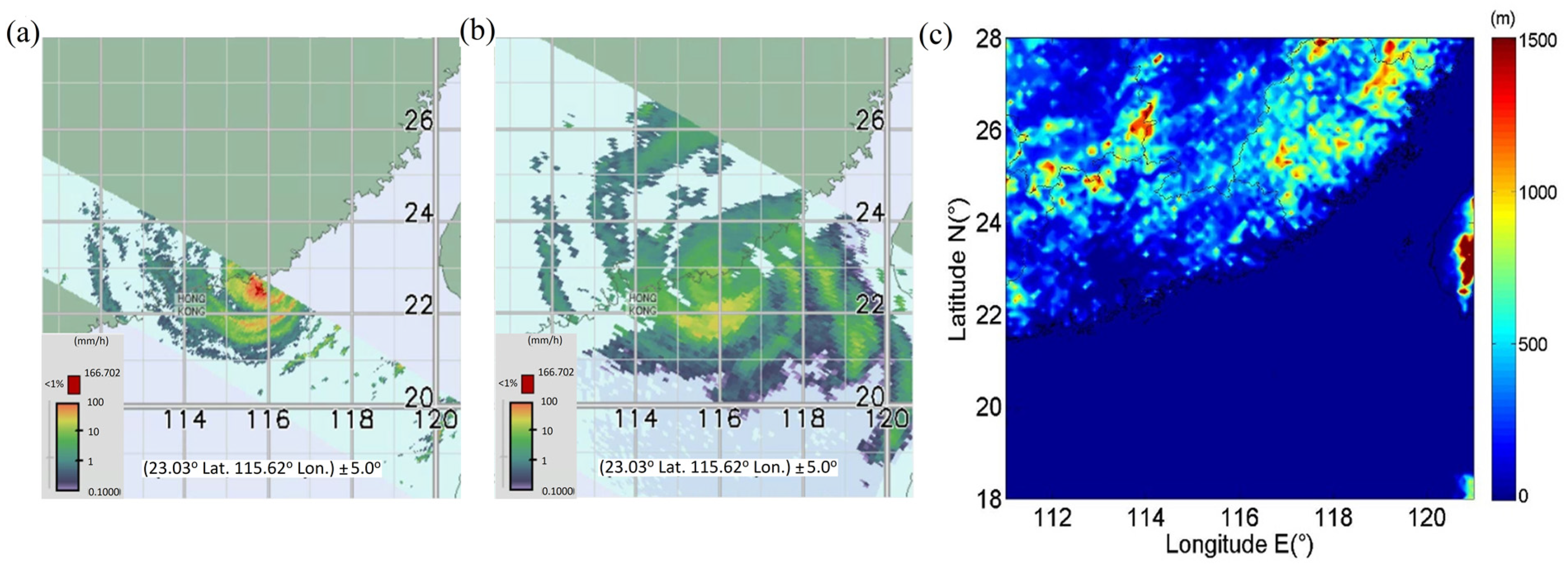
Two samples of snapshots of the rainfall fields, one from PR-TRMM and the other from TMI-TRMM, are shown in Figure 1a,b. The digital elevation maps corresponding to the sites for the snapshots are shown in Figure 1c. These digital elevation maps are downloaded from the NASA Shuttle Radar Topographic Mission (http://srtm.csi.cgiar.org/srtmdata/, accessed on 22 April 2022). In fact, the digital elevation map for the entire coastal region of mainland China is downloaded from the same website and used in the present study.
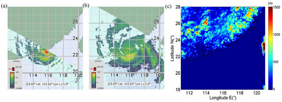
Figure 1.
Snapshots of instantaneous rainfall intensity fields (extracted from TRMM) and the corresponding digital elevation map: (a) snapshot for 23 July 2014, at latitude = 26.20°, and longitude = 118.23°; the track and wind field parameter corresponding to the snapshot are the Holland B parameter equal to 1.26, Rmax = 37.79 (km), central difference pressure Δp = 20.44 (hPa), translation velocity |uc| = 6.34 (m/s) and Intensity Category (IC) = 2, and translation angle equals 322.05°. (b) snapshot for 22 September 2013, at latitude = 22.65°, and longitude = 116.01°; the track and wind field parameter corresponding to the snapshot are the Holland B parameter equal to 1.61, Rmax = 13.38 (km), central difference pressure Δp = 78.38 (hPa), translation velocity |uc| = 7.13 (m/s) and Intensity Category (IC) = 6, and translation angle equals 286.19°, and (c) digital elevation map corresponds to the snapshots shown in (a,b).
The snapshots such as those shown in Figure 1 may contain measurement errors. Since the quantification of the error for a given snapshot of the rainfall field is unknown, such an error is neglected in the present study.
3. Calibrating PHRaM Using Snapshots of Rainfall Intensity Fields
3.1. Modeling of the Rainfall Intensity
PHRaM [22] is a modified version of the R-CLIPER model [16] by including the effect of wind shear [14] and the orographic effect. PHRaM can be written as
where (mm/h) is the predicted instantaneous rainfall intensity at a site, which is defined by a distance to the TC center r (km) and an azimuth angle α with respect to the translation direction (clockwise angle is taken as positive). In Equation (1), (mm/h) represents the predicted instantaneous rainfall intensity (i.e., predicted by the R-CLIPER model), which is an axisymmetric field. (mm/h) represents the asymmetric component of the rainfall caused by wind shear, which could be viewed as Fourier decomposition of the rainfall field with order greater than zero and conditioned on r. (mm/h) is used to take into account the effect of topographic change (i.e., the slope of the mountains).
The R-CLIPER model considers that the rainfall intensity at a distance r from the TC center can be evaluated based on
where I0 and Im are the rainfall intensity at r equal to zero and rm, respectively, rm is the radius of maximum rainfall intensity, and re is a model parameter. Based on statistical analysis results, it was suggested in [16] suggested that I0, Im, rm, and re, can be treated as linear functions of the surface wind speed (i.e., maximum wind speed at 10 m height above the ground surface of the TC event), Vm (m/s).
The asymmetric component of the rainfall intensity caused by wind shear, , is expressed as
where ak(r) and bk(r) are the Fourier series coefficients for a given r, and N is the total number of wavenumbers to be considered. It was recommended in [22] that N = 2 is to be used for model development.
The term for the topographic effects is given by
where c is a model coefficient, (m) is the ground elevation, and (m/s) represents the wind field at 10 m height above the ground surface. Further discussions on the modeling of were presented in [23,30]. Based on these studies, can be modeled using
where
where the lift (m) is the magnitude of the difference in the elevation. It was pointed out in [22,23,30] that the coefficients in Equation (5) are calculated based on a resolution of 10 km for the digital elevation map. If a different resolution is considered, the coefficient in Equation (5) (i.e., c in Equation (4)) should be re-calibrated.
It was suggested in [22] that the tangential wind velocity is to be modeled using the model given in [31]. Rather than using this suggested wind field model, in the present study, the use of the surface wind obtained by scaling the gradient wind [32] is considered. The consideration of a scaled gradient wind field could be justified since it provides a good estimate of the surface wind, as shown in [33,34,35]. Based on these studies and for the numerical analysis to be carried out in the present study, it is considered that could be approximated using
for onshore sites, where is a coefficient relating the gradient wind and surface wind velocity (in the tangential direction),
in which (m/s) is the translational velocity, ρ is the air density that can be taken equal to 1.15 (kg/m3), B is Holland’s radial pressure model parameter, Δp is the central pressure difference, Rmax is the radius to maximum wind speed, fc (rad/s) is Coriolis parameter, and α is the azimuth angle with respect to the TC translation direction and taken as positive if it is clockwise. If is assumed to be a constant, the adoption of Equations (7) and (8) also implies that , where and e is the mathematical constant that approximately equals 2.718. Based on [33,35], a value of equal to 0.83 is considered, and Vm is used to represent the 2 min mean wind speed at 10 m height above the ground surface.
The analysis presented in [13] was carried out for three TC intensity classes: tropical storms; Saffir–Simpson category-1 and -2 hurricanes; and Saffir–Simpson category-3, -4, and -5 hurricanes. Since CMA [36] classifies the intensity of TC as shown in Table 1, in the following numerical analysis, the calibration of the PHRaM for landfalling TCs affecting mainland China is carried out for three groups of intensity class: Group 1 contains IC 1, Group 2 contains IC 2 and 3, and Group 3 contains IC 4, 5, and 6. For easy reference, these three groups are referred to as GC1, GC2, and GC3, respectively.

Table 1.
Intensity Category according to CMA (https://data.cma.cn/en, accessed on 22 April 2022) [36].
3.2. Estimating Model Parameters
From the discussion presented in the previous section, it can be observed that the term is proportional to I0(r) (i.e., the R-CLIPER model) which is unknown a priori. Also, is to be estimated based on the available observed rainfall intensity field. To estimate the parameters Im, I0, rm, and re shown in Equation (2) for a given set of observed rainfall fields , we could minimize the error defined as,
where k denotes the k-th rainfall intensity field, and j denotes the j-th location of the measured rainfall intensity. However, rather than following [16] and adopting Equation (2), a modified version of Equation (2) given in the following,
is adopted in the present study, where n and ρe are model parameters. Moreover, rather than considering that Im, I0, rm, and ρe are linear functions of Vm [16], we assume , and , where a and b with subscripts and ρe are model parameters to be estimated by minimizing E0 defined in Equation (9). For simplicity, rm is taken equal to Rmax. This could be justified considering Rmax is greater than the radius where the maximum wind shear occurs and an outward radial displacement of 7.8 km that is caused by the outward wall updraft of the tropical cyclones [17]. Note that by considering the relation between Vm and Vmax, one could easily write , and if the parametrization is based on Vm.
First, the minimization of E0 shown in Equation (9) was carried out. However, on occasion, this resulted in an unrealistic prediction of rainfall intensity (i.e., extremely large value or negative value of rainfall intensity). Consequently, the parameter estimation is carried out based on the azimuthally averaged rainfall intensity calculated from the snapshots of the rainfall intensity, and the constraint that I0 is greater than zero is imposed. In such a case, Equations (9) and (10) become
where is the azimuthally averaged rainfall intensity for the k-th snapshot and the j-th annulus with a radius between , represents the averaged topographic effect for the k-th snapshot and the j-th annulus, and represents the predicted rainfall intensity. Note that rj = 10j km and = 5 km are considered to evaluate the azimuthally averaged rainfall intensity.
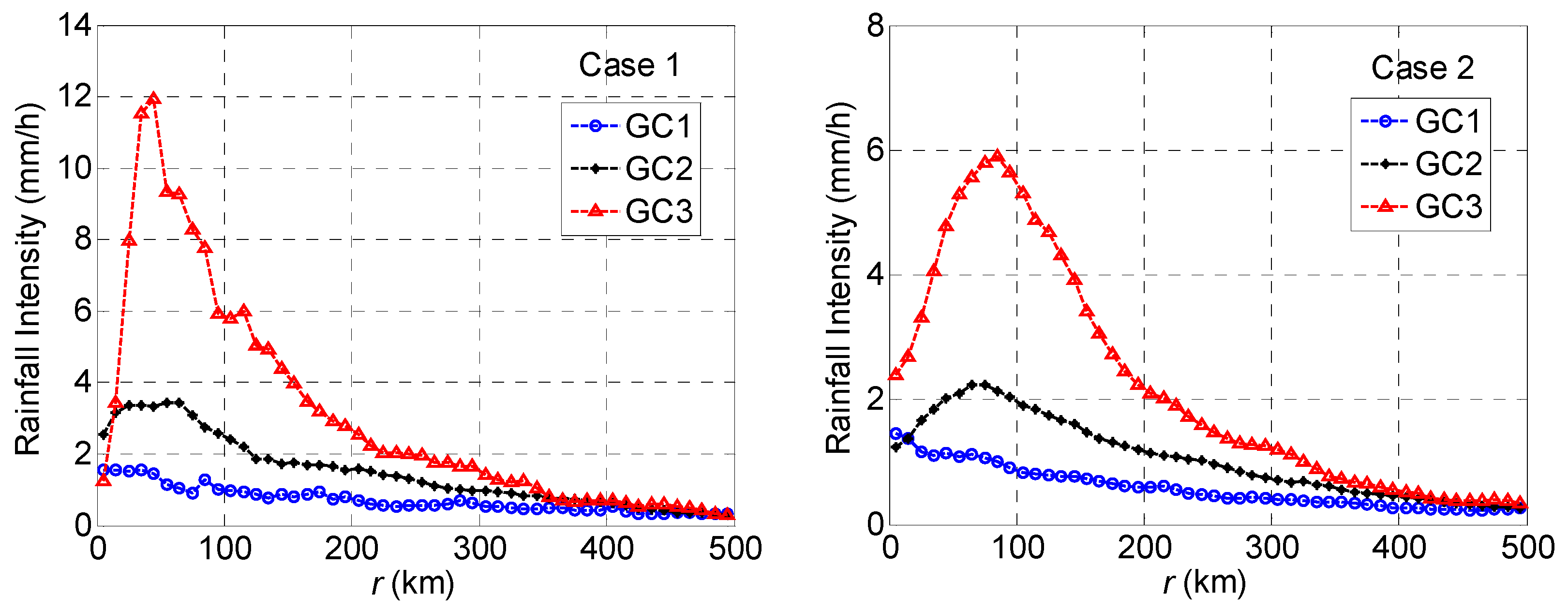
To appreciate the average behavior of the rainfall intensity, the calculated azimuthally averaged rainfall intensity is shown in Figure 2 by considering the snapshots of the rainfall fields for Case 1 and Case 2. Case 1 refers to the consideration of the 614 snapshots of the rainfall fields extracted from PR-TRMM, and Case 2 refers to the consideration of the 933 snapshots of the rainfall fields extracted from TMI-TRMM, where the extraction is discussed earlier, and details of the extracted snapshots are described in [29]. Note that since not all snapshots of the rainfall intensity have the same spatial coverage, the obtained mean for different r/rm may contain a different number of samples. The figure indicates that the mean of the rainfall intensity obtained based on PR-TRMM is greater than that obtained by using TMI-TRMM. This is consistent with the remark made in [21], indicating that PR and TMI detect different aspects of rainfall, as mentioned earlier. The obtained mean values are also consistent with those reported in [25] for areas located in the coastal region in mainland China.
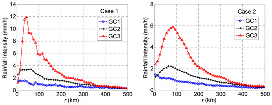
Figure 2.
Average rainfall intensity and predicted rainfall intensity.
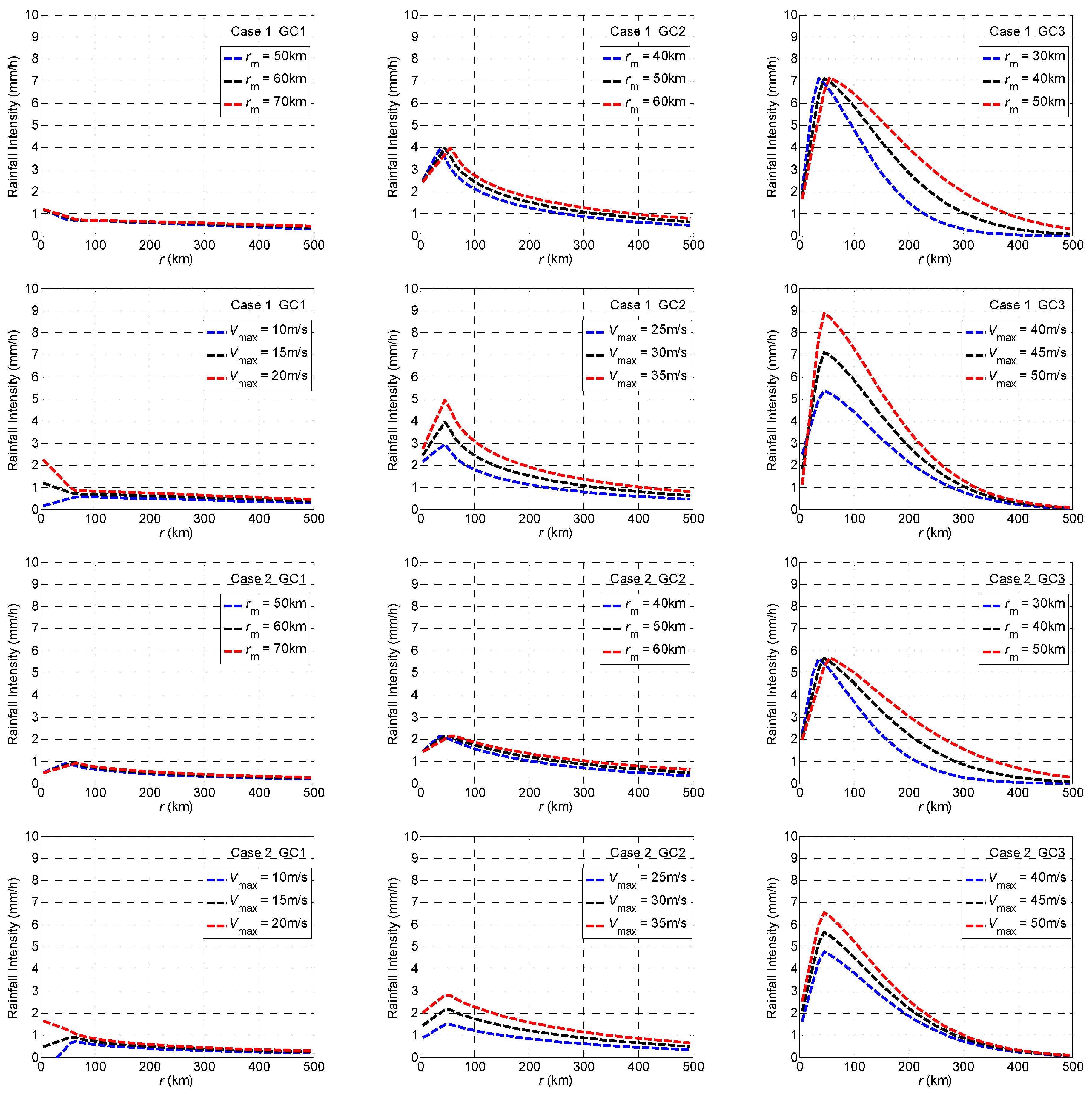
By minimizing the error defined in Equation (9), the obtained model parameters are shown in Table 2 for the grouped intensity categories (i.e., GC1, GC2, and GC3) and different cases. Based on the estimated model parameters, the predicted rainfall intensity is shown in Figure 3 for selected values of Rmax and Vmax. Since the mean presented in Figure 2 for GC1, GC2, and GC3 is obtained by considering TCs with different Rmax and Vmax (and snapshots with incomplete coverage of the rainfall intensity field), the results shown in Figure 2 and Figure 3 should not be compared quantitatively. However, the qualitative trends of the rainfall intensity in the radial direction shown in Figure 2 and Figure 3 are consistent. Also, the results shown in Figure 2 indicate that the predicted rainfall intensity is sensitive to Rmax and Vmax. An increase in Rmax and Vmax leads to increased predicted azimuthally average rainfall intensity. In all cases, the use of the model parameters developed based on TMI-TRMM leads to the predicted azimuthally averaged rainfall intensity that is less than the one predicted using the model developed based on PR-TRMM. However, it must be emphasized that the predicted rainfall accumulation by considering the passage of a TC event depends on the azimuthally averaged rainfall intensity and the asymmetric component of the rainfall intensity.
Table 2.
Estimated model coefficient for the mean rainfall intensity (see Equation (10)).
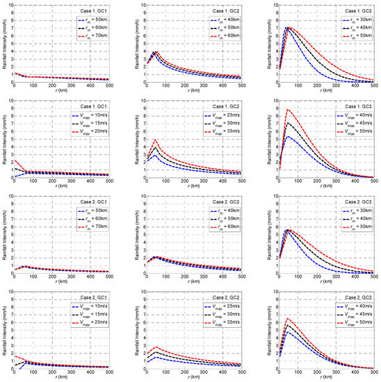
Figure 3.
Predicted azimuthally averaged rainfall intensity using the model parameters shown in Table 2. For the plots where Vmax is shown, rm equals 60, 50, and 40 km for GC1, GC2, and GC3, respectively. For the plots where rm is shown, Rmax equals 15, 30, and 45 m/s for GC1, GC2, and GC3, respectively.
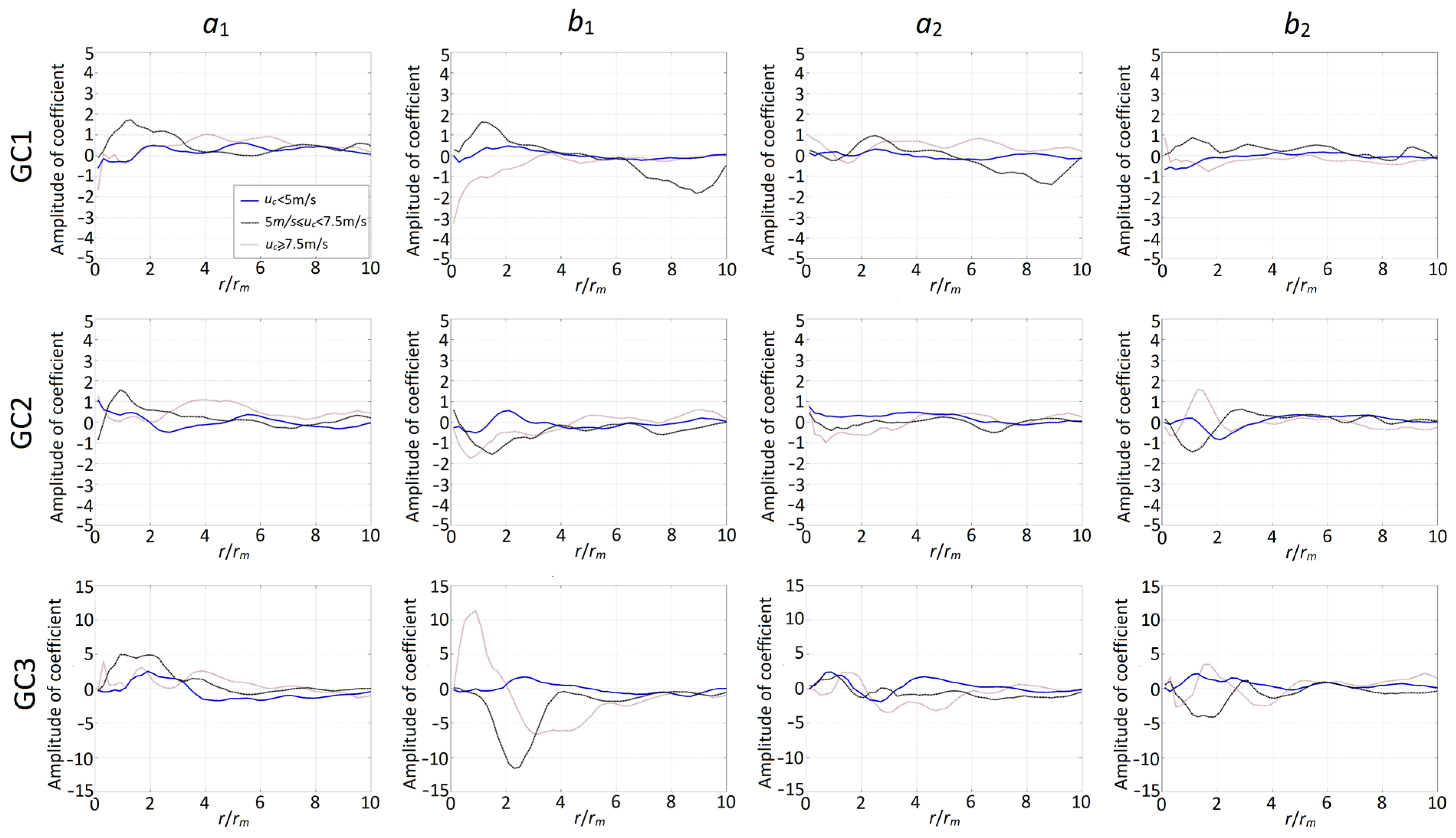
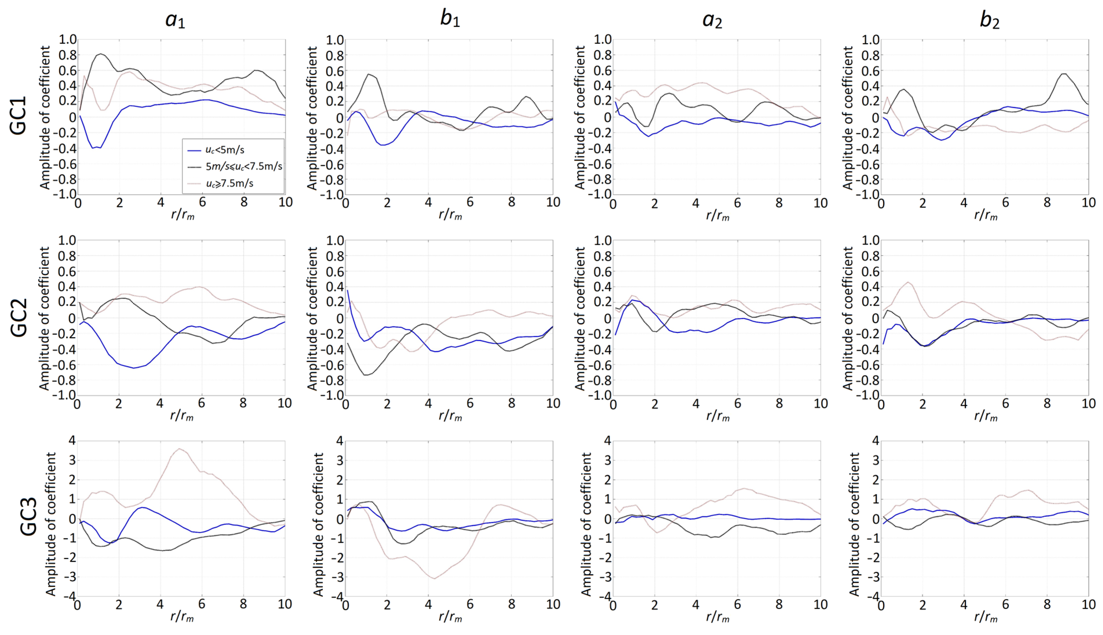
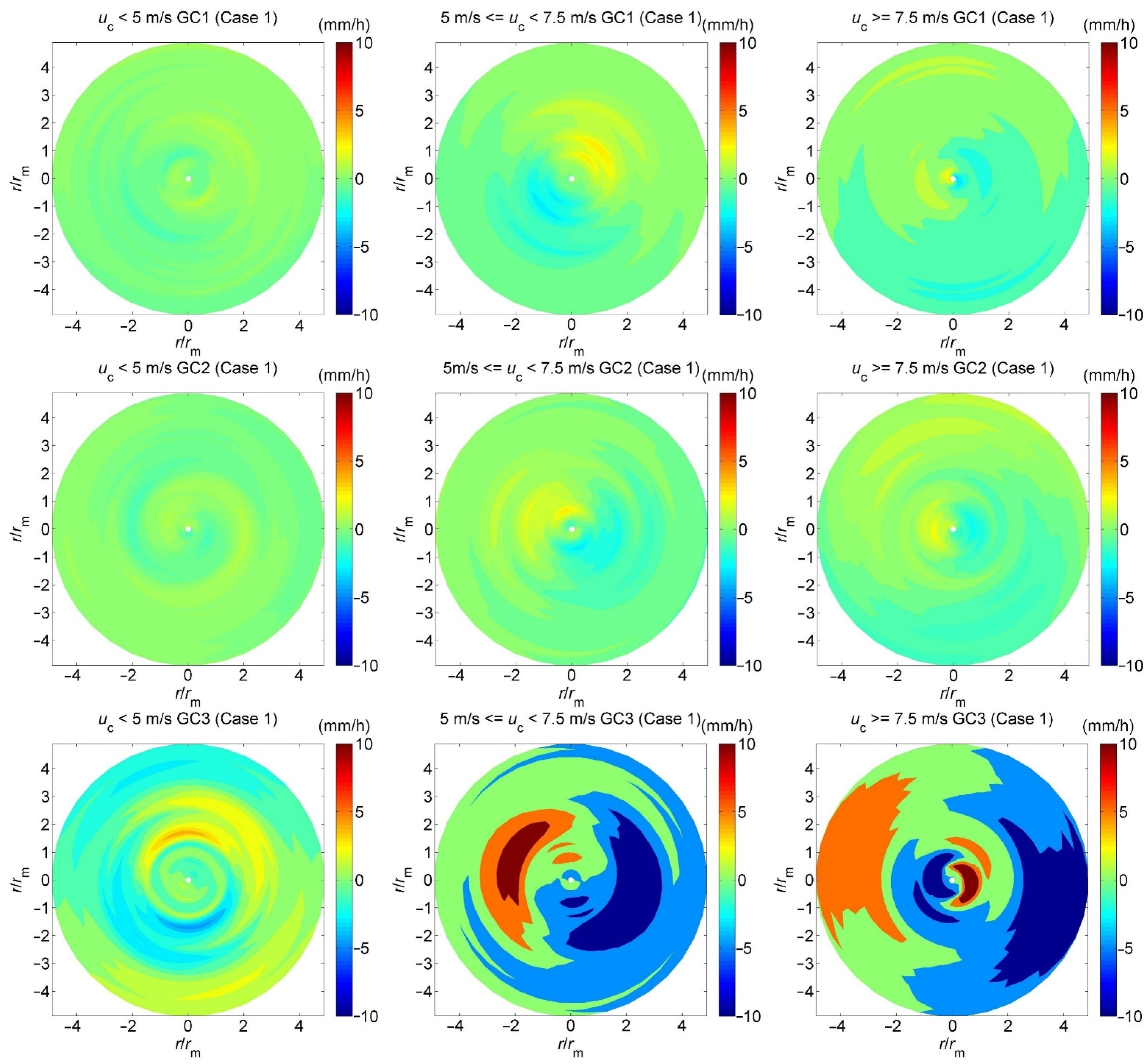
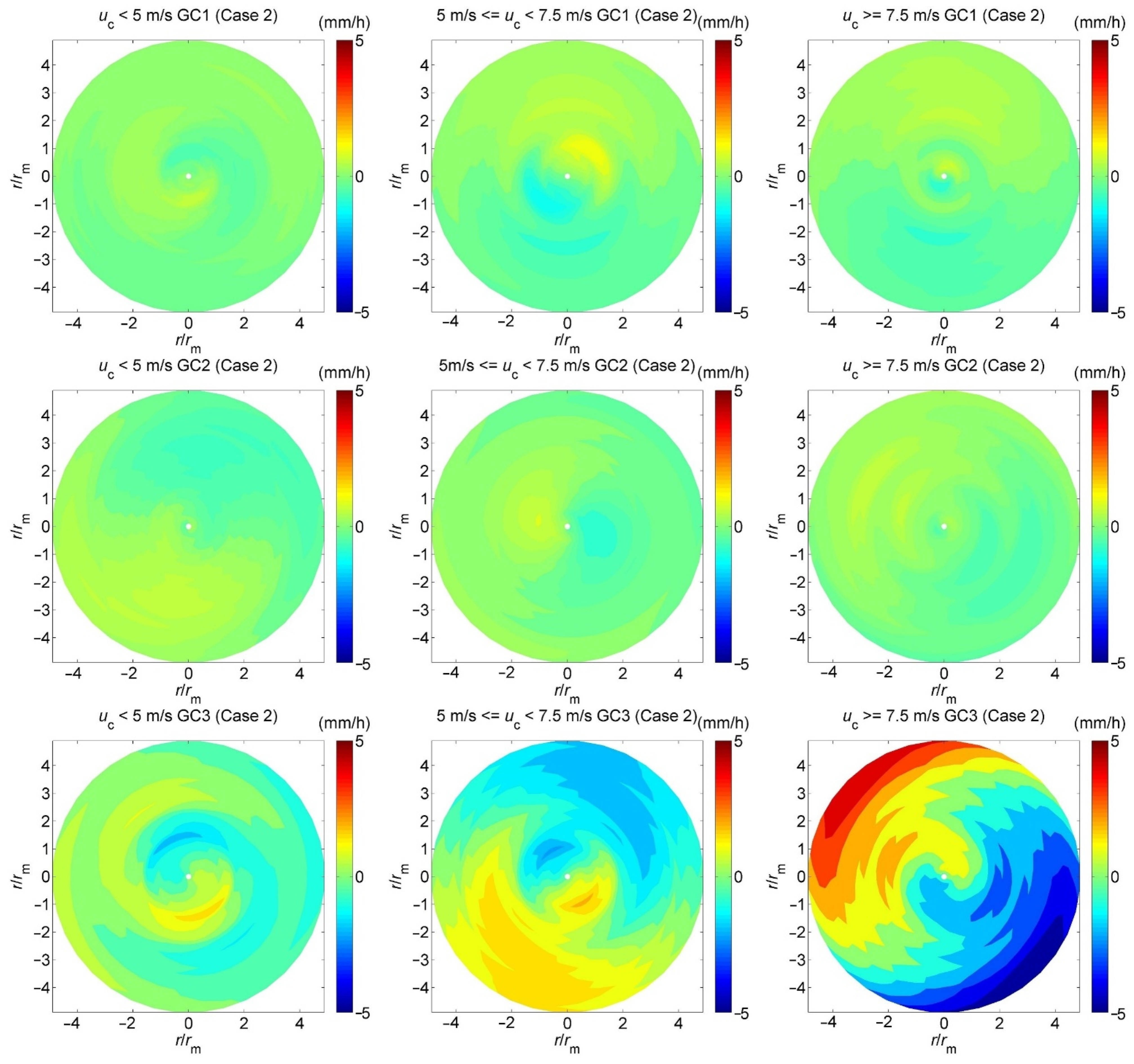
To assess the asymmetric component of the rainfall intensity field, we retain the terms associated with wavenumber 1 and 2 to represent , as shown in Equation (3), but replace the Fourier coefficients ak(r) and bk(r) with ak(r/rm) and bk(r/rm). This replacement is consistent with the parametrization used for I0(r) shown in Equation (10). The Fourier coefficients can be calculated using and the Fourier series properties. The resulting coefficients for GC1, GC2, and CG3 are shown in Figure 4 and Figure 5 for Case 1 and Case 2, respectively. The figures show that the Fourier coefficients vary radially and depend on the grouped intensity categories. For each case, the largest amplitude of the Fourier coefficients occurs for GC3, indicating that the asymmetric rainfall intensity for GC3 is likely to be more severe than that for GC1 and GC2.
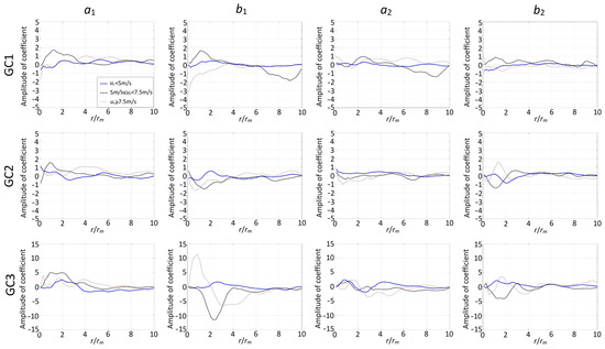
Figure 4.
Coefficients for the asymmetric rainfall intensity field for Case 1. The first to third rows correspond to GC1 to GC3, respectively. ak(r/rm) and bk(r/rm) has units of mm/h, where k = 1 and 2.
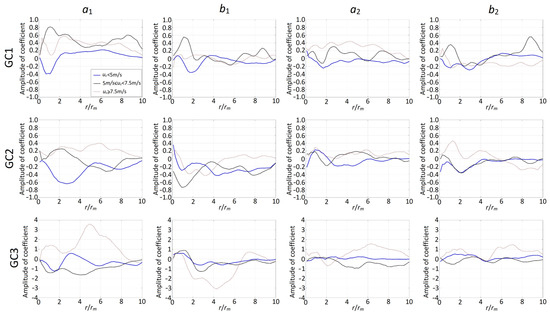
Figure 5.
Coefficients for the asymmetric rainfall intensity field for Case 2. The first to third rows correspond to GC1 to GC3, respectively. ak(r/rm) and bk(r/rm) has units of mm/h, where k = 1 and 2.
To appreciate the asymmetric rainfall field, we plot using the obtained Fourier coefficients shown in Figure 4 and Figure 5. The obtained results are shown in Figure 6 and Figure 7 for Cases 1 and 2. The figures indicate that there is a strong asymmetric component in the rainfall intensity fields. This observation is consistent with those reported in [14,22,25]. The obtained magnitude of the asymmetry shown in Figure 6 and Figure 7 differs from those presented in [25]. This is partly due to that the obtained asymmetry is affected by selected snapshots, topographic effect, and, possibly, regional influence. Also, the study by [25] was focused on the asymmetry of the rainfall intensity for selected coastal provinces and for the TCs before and after landfall. In all cases, the asymmetric depends on whether the data from PR-TRMM or TMI-TRMM are used. The asymmetry obtained by using the data from PR-TRMM is stronger than that obtained by using the data from TMI-TRMM.
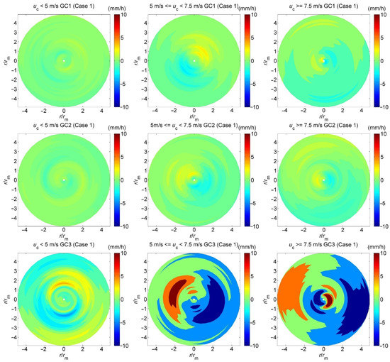
Figure 6.
Asymmetric rainfall fields calculated based on the model coefficients shown in Figure 4 for Case 1.
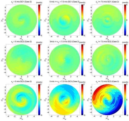
Figure 7.
Asymmetric rainfall fields calculated based on the model coefficients shown in Figure 5 for Case 2.
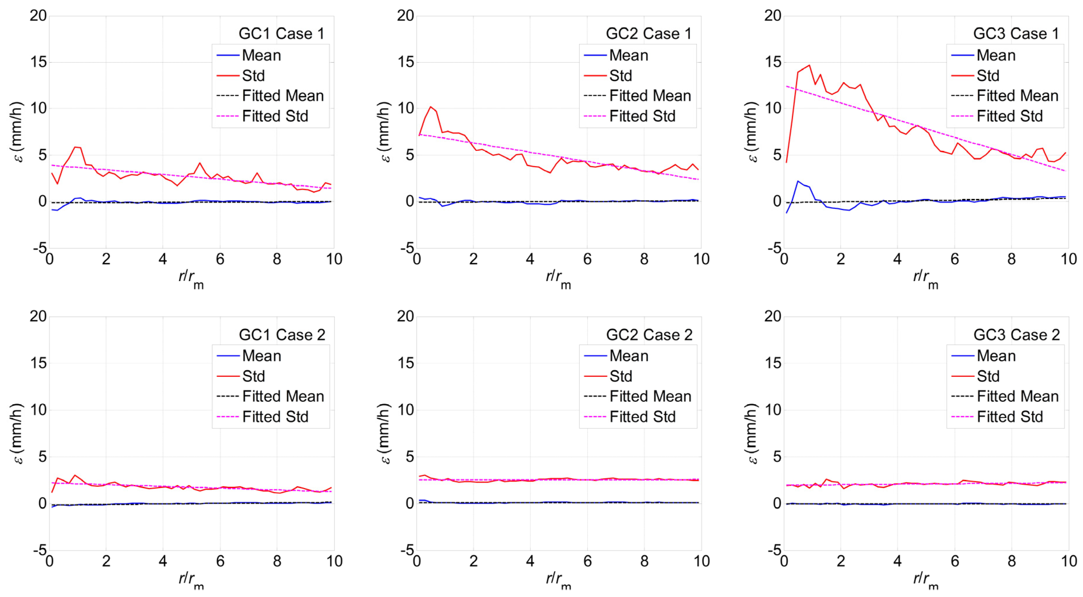
By using the developed models and the considered snapshots, the mean and standard deviation of the residuals, ε(r/rm), are calculated and shown in Figure 8. Part of this residual is due to the consideration of only the first two wavenumbers in the Fourier series expansion. The results shown in Figure 8 indicate that the mean is near zero, indicating that the developed empirical model for the rainfall intensity is almost unbiased. In addition, the standard deviation decreases as r/rm increases. The decrease in the standard deviation can be explained by noting that the rainfall intensity decreases as ε(r/rm). The mean and standard deviation may be approximated by a linear function as shown in Figure 8 with the parameters given in Table 3.
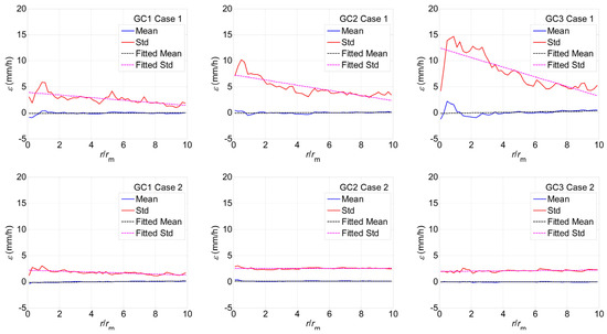
Figure 8.
Mean and standard deviation of residual ε(r/rm).
Table 3.
Parameters for the statistics of the residuals.
Based on the above, in summary, the developed rainfall intensity model is given by
where the axisymmetric component is given by Equation (10) with model parameters presented in Table 2 that depend on the adopted data (PR or TMI) and the considered intensity category, , is presented in Equation (6), which depends on the topography and the TC wind field, , and are the coefficients shown in Figure 4 and Figure 5, and the residual is assumed to be normally distributed with mean and standard deviation defined in Table 3. Note that the analysis of the spatial interevent correlation and intraevent correlation of the residuals is beyond the scope of the present study, although it can be important for mapping TC rainfall hazard for an area. This aspect should be scrutinized in a future study.
4. Evaluation of the TC Rain Hazard
4.1. Procedure to Estimate the Accumulated Rainfall at a Single Site
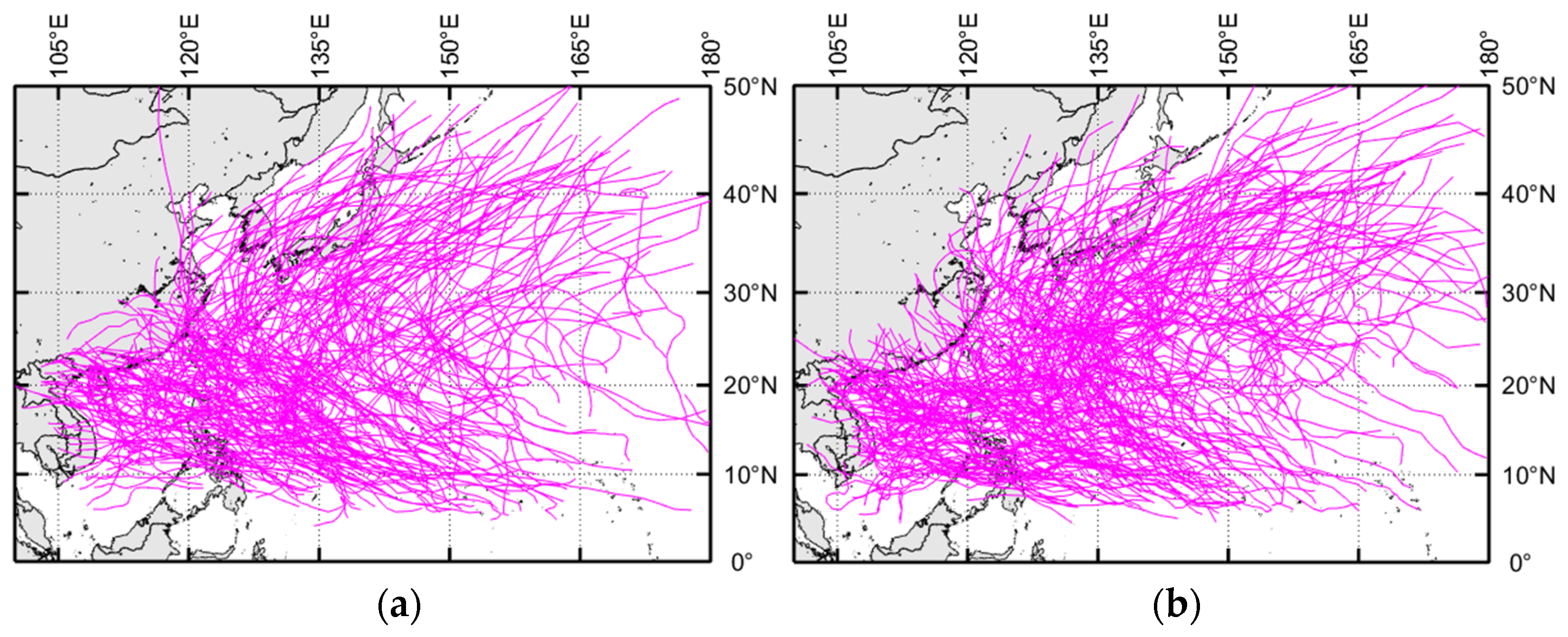
The modeling of the (instantaneous) TC rainfall intensity presented in the previous section depends on the parameters Rmax, Vmax, B, and (i.e., translation velocity and the translation direction). These parameters are available or can be calculated based on the information given in the historical TC tracks [10] or synthetic tracks [8]. In both cases, the information on TC tracks is given every 6 h, providing the time, location (latitude and longitude), and the minimum pressure near the TC center. An example of the historical TC and synthetic TC activities for a period of 10 years is shown in Figure 9. It is observed that the total number of landfalling TCs based on the historical catalogue is 75, agreeing with the observation that the annual average number of landfalling TCs in mainland China is about 8 [5].
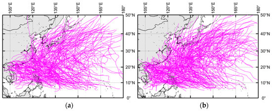
Figure 9.
Illustration of the TC tracks for a period of 10 years: (a) Using historical TC tracks from 2001 to 2010 based on the historical catalogue given in Ying et al. (2014) and (b) Using synthetic TC tracks generated by applying the model given in Li and Hong (2016) for a period of 10 years.
Note that the time and location of the track can be used to evaluate . The minimum pressure near the TC center can be employed to evaluate the central pressure difference Δp. If Rmax and B can be evaluated using [37],
and,
where Δp is in hPa, ψ is the latitude, the standard deviation of , equals 0.448 for , for , and 0.186 for ; and the standard deviation of εB, σB, equals 0.221. Note that the adequacy of using Rmax and B for assessing the TC wind hazard for mainland China has been shown in [8,35,38,39].
The assessment of the accumulated rainfall at a site caused by the passing of a TC requires considering the time-varying characteristics of the TC tracks. A TC track that is given every 6 h is interpolated along the track every 15 min. Based on these calculated parameters for a given TC at a given instance (i.e., Δp, location, and ), Rmax and B are calculated by using Equations (13) and (14). By using Rmax, B, Δp, and , and the adopted simple wind field shown in Equations (7) and (8), the gradient wind , the surface wind field , Vmax, and Vm are calculated. The value of Vm is to be used to determine the intensity category of the TC at the considered time instance (i.e., whether the TC at the considered instance belongs to GC1, GC2, or GC3). The identification of the intensity category is necessary for selecting the model parameters to evaluate I0(r) (see Equation (10)). The wind field is used to evaluate the coefficient for the topographic effect described in Equation (6). The predicted rainfall intensity at the considered instance is then calculated using Equation (12). The accumulated rainfall is obtained by integrating the rainfall intensity at each 15 min time step over the time interval of the TC that affects the site.
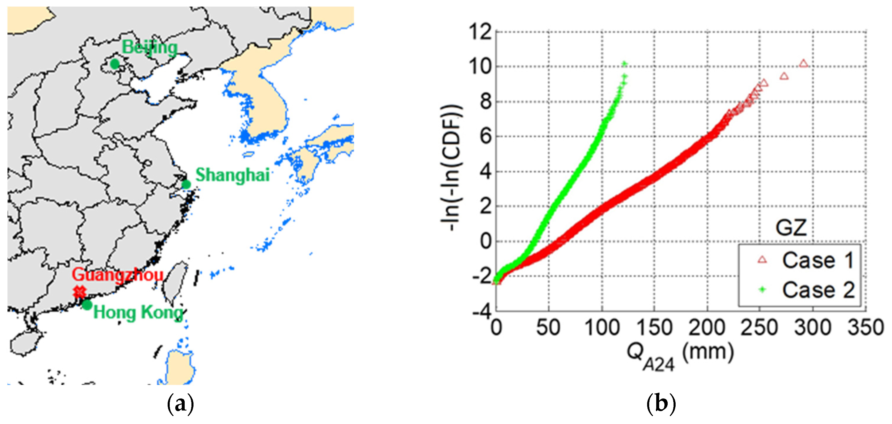
As an illustration, the above-outlined procedure is used to assess the accumulated rain hazard by using the synthetic tracks for a period of 25,000 years. For the assessment, the site (i.e., Guangzhou referred to as GZ) shown in Figure 10a, and the rainfall intensity model for Case 1 (i.e., based on the data from PR-TRMM) is considered. The assessed maximum accumulated rain per 24 h, Q24, that is caused by each TC for the site (i.e., Guangzhou) is evaluated. The annual maximum of Q24, denoted as QA24, is extracted from the samples for each year and is presented in Figure 10b.
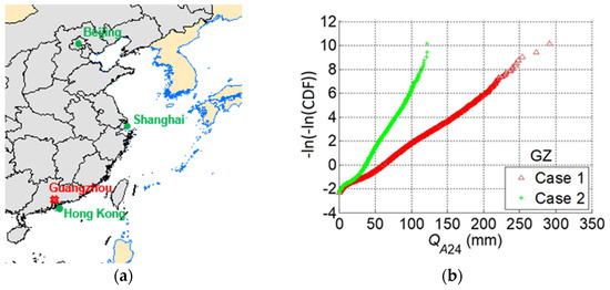
Figure 10.
Considered site and empirical distribution of the maximum accumulated rainfall for 24 h: (a) considered site and (b) empirical probability distribution of QA24 presented in the Gumbel probability paper, where the vertical axis represents the value of -ln (-ln(CDF)) in which CDF denotes the value of the (empirical) cumulative probability distribution function (CDF).
The analysis that is carried out is repeated but considering the rainfall model for Case 2. The results are compared in Figure 10b. QA24 estimated based on Case 1 is about 60% greater than that estimated based on Case 2. In other words, the use of the rainfall model developed based on PR-TRMM leads to the estimated QA24 that is about 60% greater than that obtained by using the rainfall model developed based on TMI-TRMM.
4.2. TC Rain Hazard Mapping
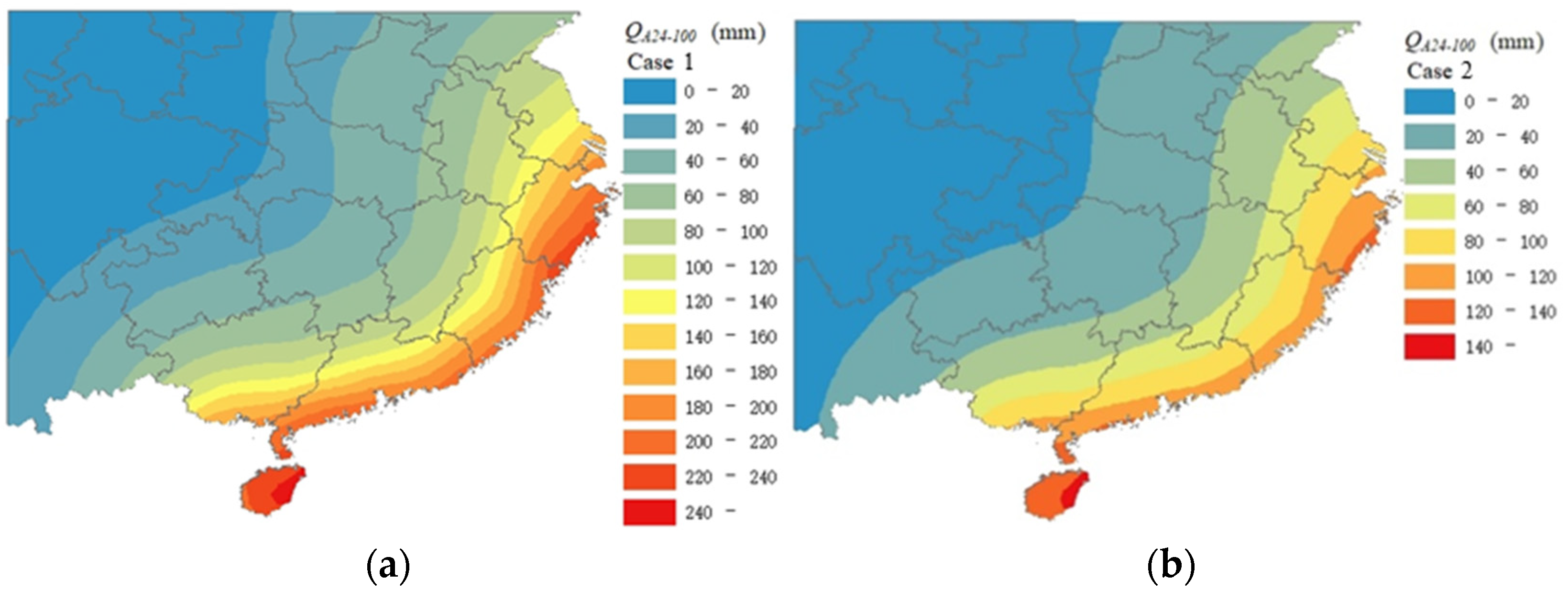
To map the rain hazard, we consider the square grid system with the distance between the grid of 0.5° covering the coastal region in mainland China. We carry out the analysis that is presented in the previous section but for each point within the grid system.
The obtained results are presented in Figure 11. The results indicate that the obtained values for Case 1 are greater than those for Case 2. The ratio of the former to the latter is about 1.6, which is consistent with that observed in Figure 10 for Guangzhou. However, this is greater than that inferred from Figure 9 (i.e., I0(r)), which is about 1.4. This discrepancy may be explained by noting that the standard deviation of the residual for Case 1 is about twice that for Case 2. The standard deviation also affects the estimated extreme value of the accumulated rain hazard.

Figure 11.
Mapped accumulated annual maximum rainfall hazard: (a) 100-year return period value of QA24 if rainfall intensity model for Case 1 is used and (b) 100-year return period value of QA24 if rainfall intensity model for Case 2 is used.
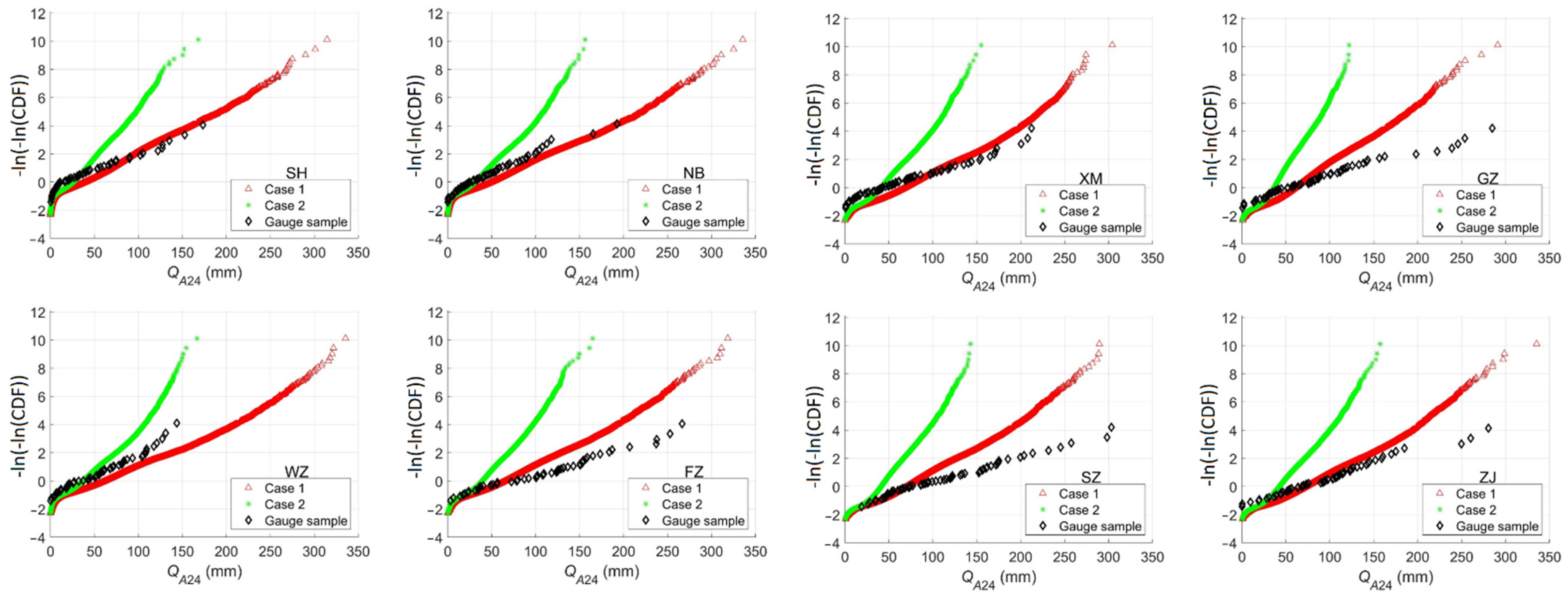
4.3. Comparison with Estimation from Gauge Data
An attempt to validate the developed models is carried out by comparing the estimated accumulated rain hazard using the developed model and simulation framework to that estimated based on gauge data for a few selected cities that are listed in Table 4. The gauge data are obtained from CMA website (https://data.cma.cn/en, accessed on 22 April 2022) for the meteorological stations located in the selected cities. Based on the historical gauge record and the best TC track dataset [10], we identified the recorded rain associated with TC events. We calculated the samples of QA24 for each considered site listed in Table 4. The samples of QA24 are shown in Figure 12 in the Gumbel probability paper for each considered site. Also, the simulation analysis of QA24 for each considered site is carried out using the developed rainfall intensity model and simulated TC tracks as was done in the previous section. The samples of QA24 are also shown in Figure 12. The estimated 100-year return period values of QA24 based on the empirical distributions shown in Figure 12 are summarized in Table 4. The comparison shown in Figure 12 and Table 4 indicates that the accumulated rain hazard obtained by using the developed model and simulation procedure is less than that obtained based on the gauge data, except for Wenzhou. QA24 based on the gauge data is estimated by fitting the samples using the Gumbel distribution and the least-squares method. The ratio of QA24 obtained based on the developed models to that estimated based on the gauge data is not consistent. This inconsistency could arise from several sources, including the measurement error associated with gauge data and the extrapolation through the distribution fitting. On average, the ratio of QA24 estimated based on Case 1 to that estimated based on the gauge data equals is about 76.4%, and the ratio of QA24 estimated based on Case 2 to that estimated based on the gauge data is about 47.3%. Note that the average of the ratio of the estimated QA24 based on the gauge data to that estimated based on Case 1 equals 1.41 and the average of the ratio of the estimated QA24 based on the gauge data to that estimated based on Case 2 equals 2.28. These values are not equal to 1/0.764 and 1/0.473 because the expectation of 1/X is not equal to 1 divided by the expectation of X. The observations reflect the fact that the snapshots from TRMM that are used to develop the TC rainfall intensity models under-estimate the actual TC rainfall intensity [17,22].
Table 4.
Comparison of the estimated accumulated rain hazard.
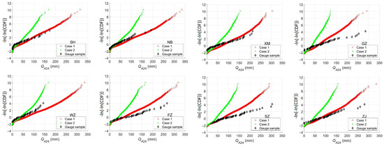
Figure 12.
Comparison of QA24 due to TC rainfall for selected sites on the Gumbel probability paper, where the vertical axis represents the value of −ln (−ln(CDF)) in which CDF denotes the value of the (empirical) cumulative probability distribution function (CDF).
5. Conclusions
We use the rainfall intensity fields from PR-TRMM and TMI-TRMM to evaluate the parameters for the TC rainfall intensity model (i.e., PHRaM) for the TCs affecting onshore sites in the coastal region of mainland China. To show the application of the models for the TC rain hazard assessment, we combine the developed rainfall intensity models, and synthetic TC tracks to estimate the T-year return period value of the accumulated rainfall per 24 h, QA24-T. We mapped QA24-100 for part of the coastal region in mainland China. These maps show that the spatial variation of QA24-100 is relatively smooth. Also, the estimated QA24-100 using models developed based on the snapshots from PR-TRMM is about 60% of that obtained using models developed based on the snapshots from TMI-TRMM. This inconsistency reflects the differences in the rainfall intensities reported by TMI-TRMM and PR-TRMM.
Moreover, as part of verification, we compare the estimated QA24-100 from surface meteorological stations at a few sites to those estimated using the developed models and synthetic TC tracks. The comparison indicates that, on average, QA24-100 based on gauge data is about 1.4 times that obtained using the model developed based on the snapshots from PR-TRMM, and about 2.3 times that obtained using the model developed based on the snapshots from TMI-TRMM. This suggests that one may consider a scaling factor of 1.4 for the rainfall intensity model developed based on snapshots from PR-TRMM and a scaling factor of 2.3 for the rainfall intensity model developed based on snapshots from TMI-TRMM. By including these scaling factors, the estimated accumulated rain hazard by using the empirical models and synthetic TC tracks could be consistent with that estimated based on records from gauge data.
Author Contributions
Conceptualization, J.G. and H.H.; methodology, J.G., X.C. and H.H.; software, J.G. and X.C.; validation, J.G., X.C. and H.H.; formal analysis, J.G., X.C. and H.H.; investigation, J.G., X.C. and H.H.; resources, H.H.; writing—original draft preparation, J.G. and H.H.; writing—review and editing, J.G., X.C. and H.H.; visualization, J.G. and X.C.; supervision, H.H.; project administration, H.H.; funding acquisition, H.H. All authors have read and agreed to the published version of the manuscript.
Funding
This research was funded by the Natural Sciences and Engineering Research Council of Canada (grant number RGPIN-2016-04814) for HPH; and the University of Western Ontario.
Institutional Review Board Statement
Not applicable.
Informed Consent Statement
Not applicable.
Conflicts of Interest
The authors declare no conflict of interest.
References
- Luo, Y.; Sun, J.; Li, Y.; Xia, R.; Du, Y.; Yang, S.; Zhang, Y.; Chen, J.; Dai, K.; Shen, X.; et al. Science and prediction of heavy rainfall over China: Research progress since the reform and opening-up of new China. J. Meteorol. Res. 2020, 34, 427–459. [Google Scholar] [CrossRef]
- Chen, L.; Li, Y.; Cheng, Z. An overview of research and forecasting on rainfall associated with landfalling tropical cyclones. Adv. Atmos. Sci. 2010, 27, 967–976. [Google Scholar] [CrossRef]
- Zhang, Q.; Wu, L.; Liu, Q. Tropical cyclone damage in China: 1983–2006. Bull. Am. Meteorol. Soc. 2009, 90, 489–495. [Google Scholar] [CrossRef] [Green Version]
- Xiao, F.; Xiao, Z. Characteristics of tropical cyclones in China and their impacts analysis. Nat. Hazards 2010, 54, 827–837. [Google Scholar]
- Hong, H.P.; Li, S.H.; Duan, Z.D. Typhoon wind hazard estimation and mapping for coastal region in mainland China. Nat Hazards Rev. 2016, 17, 04016001. [Google Scholar] [CrossRef]
- Sun, J.H.; Qi, L.L.; Zhao, S.X. A study on mesoscale convective systems of the severe heavy rainfall in North China by “9608” typhoon. Acta Meteor. Sin. 2006, 64, 57–71. (In Chinese) [Google Scholar] [CrossRef]
- Xiao, Y.F.; Duan, Z.D.; Xiao, Y.Q.; Ou, J.P.; Chang, L.; Li, Q.S. Typhoon wind hazard analysis for southeast China coastal regions. Struct. Saf. 2011, 33, 286–295. [Google Scholar] [CrossRef]
- Li, S.H.; Hong, H.P. Typhoon wind hazard estimation for China using an empirical track model. Nat. Hazards 2016, 82, 1009–1029. [Google Scholar] [CrossRef]
- Sheng, C.; Hong, H.P. On the joint tropical cyclone wind and wave hazard. Struct. Saf. 2020, 84, 101917. [Google Scholar] [CrossRef]
- Ying, M.; Zhang, W.; Yu, H.; Lu, X.; Feng, J.; Fan, Y.; Zhu, Y.; Chen, D. An overview of the China Meteorological Administration tropical cyclone database. J. Atmos. Ocean. Technol. 2014, 31, 287–301. [Google Scholar] [CrossRef] [Green Version]
- Frank, W.M.; Ritchie, E.A. Effects of vertical wind shear on the intensity and structure of numerically simulated hurricanes. Mon. Weather Rev. 2001, 129, 2249–2269. [Google Scholar] [CrossRef]
- DeMaria, M.; Tuleya, R.E. Evaluation of quantitative precipitation forecasts from the GFDL hurricane model. Preprints. In Proceedings of the Symposium on Precipitation of Extremes: Prediction, Impacts, and Responses, Alberquerque, NM, USA, 14–18 January 2001; pp. 340–343. [Google Scholar]
- Lonfat, M.; Marks, F.D., Jr.; Chen, S.S. Precipitation distribution in tropical cyclones using the Tropical Rainfall Measuring Mission (TRMM) Microwave Imager: A global perspective. Mon. Weather Rev. 2004, 132, 1645–1660. [Google Scholar] [CrossRef]
- Chen, S.S.; Knaff, J.A.; Marks, F.D., Jr. Effects of vertical wind shear and storm motion on tropical cyclone rainfall asymmetries deduced from TRMM. Mon. Weather Rev. 2006, 134, 3190–3208. [Google Scholar] [CrossRef]
- Ueno, M. Observational analysis and numerical evaluation of the effects of vertical wind shear on the rainfall asymmetry in the typhoon inner-core region. J. Meteorol. Soc. Japan. Ser. II 2007, 85, 115–136. [Google Scholar] [CrossRef] [Green Version]
- Tuleya, R.E.; DeMaria, M.; Kuligowski, R.J. Evaluation of GFDL and simple statistical model rainfall forecasts for US landfalling tropical storms. Weather Forecast. 2007, 22, 56–70. [Google Scholar] [CrossRef]
- Langousis, A.; Veneziano, D. Theoretical model of rainfall in tropical cyclones for the assessment of long-term risk. J. Geophys. Res. Atmos. 2009, 114, D02106. [Google Scholar] [CrossRef]
- Rogers, R.; Marks, F.; Marchok, T. Tropical cyclone rainfall. Encycl. Hydrol. Sci. J. 2009, 3, hsa030. [Google Scholar]
- Simpson, J.; Adler, R.F.; North, G.R. A proposed tropical rainfall measuring mission (TRMM) satellite. Bull. Am. Meteor. Soc. 1988, 69, 278–295. [Google Scholar] [CrossRef] [Green Version]
- Kummerow, C.; Simpson, J.; Thiele, O.; Barnes, W.; Chang, A.T.C.; Stocker, E.; Adler, R.F.; Hou, A.; Kakar, R.; Wentz, F.; et al. The status of the Tropical Rainfall Measuring Mission (TRMM) after two years in orbit. J. Appl. Meteorol. 2000, 39, 1965–1982. [Google Scholar] [CrossRef]
- Yamamoto, M.K.; Furuzawa, F.A.; Higuchi, A.; Nakamura, K. Comparison of diurnal variations in precipitation systems observed by TRMM PR, TMI, and VIRS. J. Clim. 2008, 21, 4011–4028. [Google Scholar] [CrossRef]
- Lonfat, M.; Rogers, R.; Marchok, T.; Marks, F.D., Jr. A parametric model for predicting hurricane rainfall. Mon. Weather Rev. 2007, 135, 3086–3097. [Google Scholar] [CrossRef]
- Brackins, J.T.; Kalyanapu, A.J. Evaluation of parametric precipitation models in reproducing tropical cyclone rainfall patterns. J. Hydrol. 2020, 580, 124255. [Google Scholar] [CrossRef]
- Yu, Z.; Wang, Y.; Xu, H. Observed rainfall asymmetry in tropical cyclones making landfall over China. J. Appl. Meteorol. Climatol. 2015, 54, 117–136. [Google Scholar] [CrossRef]
- Yu, Z.; Wang, Y.; Xu, H.; Davidson, N.; Chen, Y.; Chen, Y.; Yu, H. On the relationship between intensity and rainfall distribution in tropical cyclones making landfall over China. J. Appl. Meteorol. Climatol. 2017, 56, 2883–2901. [Google Scholar] [CrossRef]
- Lu, P.; Lin, N.; Emanuel, K.; Chavas, D.; Smith, J. Assessing hurricane rainfall mechanisms using a physics-based model: Hurricanes Isabel (2003) and Irene (2011). J. Atmos. Sci. 2018, 75, 2337–2358. [Google Scholar] [CrossRef]
- Xi, D.; Lin, N.; Smith, J. Evaluation of a physics-based tropical cyclone rainfall model for risk assessment. J. Hydrometeorol. 2020, 21, 2197–2218. [Google Scholar] [CrossRef]
- Marks, F.D.; Kappler, G.; DeMaria, M. Development of a tropical cyclone rainfall climatology and persistence (RCLIPER) model. Preprints. In Proceedings of the 25th Conference on Hurricanes and Tropical Meteorology, San Diego, CA, USA, 29 April–3 May.
- Gu, J.Y. Estimation of Tropical Cyclone Rain Hazard for Sites in Coastal Region of Mainland China. Ph.D. Thesis, The University of Western Ontario, London, ON, Canada, 2021. Available online: https://ir.lib.uwo.ca/etd/8175 (accessed on 22 April 2022).
- Grieser, J.; Jewson, S. The RMS TC-rain model. Meteorol. Z. 2012, 21, 79. [Google Scholar] [CrossRef]
- Willoughby, H.E.; Darling, R.W.R.; Rahn, M.E. Parametric representation of the primary hurricane vortex. Part II: A new family of sectionally continuous profiles. Mon. Weather Rev. 2006, 134, 1102–1120. [Google Scholar] [CrossRef] [Green Version]
- Holland, G.J. An analytic model of the wind and pressure profiles in hurricanes. Mon. Weather Rev. 1980, 108, 1212–1218. [Google Scholar] [CrossRef]
- Georgiou, P.N.; Davenport, A.G.; Vickery, B.J. Design wind speeds in regions dominated by tropical cyclones. J. Wind Eng. Ind. Aerodyn. 1983, 13, 139–152. [Google Scholar] [CrossRef]
- Young, I.R. A review of parametric descriptions of tropical cyclone wind-wave generation. Atmosphere 2017, 8, 194. [Google Scholar] [CrossRef] [Green Version]
- Gu, J.Y.; Sheng, C.; Hong, H.P. Comparison of tropical cyclone wind field models and their influence on estimated wind hazard. Wind Struct. 2020, 31, 321–334. [Google Scholar]
- GB/T19201-2006; Classification of Tropical Cyclones. China Standard Press: Beijing, China, 2006. (In Chinese)
- Vickery, P.J.; Wadhera, D. Statistical models of Holland pressure profile parameter and radius to maximum winds of hurricanes from flight-level pressure and H* Wind data. J. Appl. Meteorol. Climatol. 2008, 47, 2497–2517. [Google Scholar] [CrossRef]
- Li, S.H.; Hong, H.P. Use of historical best track data to estimate typhoon wind hazard at selected sites in China. Nat. Hazards 2015, 76, 1395–1414. [Google Scholar] [CrossRef]
- Mo, H.M.; Hong, H.P.; Li, S.H.; Fan, F. Impact of Annual Maximum Wind Speed in Mixed Wind Climates on Wind Hazard for Mainland China. Nat. Hazards Rev. 2022, 23, 04021061. [Google Scholar] [CrossRef]
Publisher’s Note: MDPI stays neutral with regard to jurisdictional claims in published maps and institutional affiliations. |
© 2022 by the authors. Licensee MDPI, Basel, Switzerland. This article is an open access article distributed under the terms and conditions of the Creative Commons Attribution (CC BY) license (https://creativecommons.org/licenses/by/4.0/).