Abstract
We present a modified model with a set of wall-functions suitable for reconstruction of sensible heat and momentum fluxes from the observations data (e.g., surface temperature evolution during the diurnal cycle). The modification takes into account stability and buoyancy effects in the Reynolds stress parametrization which affects turbulence production and turbulent heat flux. The single-cell and single-column versions of the model are presented. The model is tested based on CASES-99 observations data for dry ABL. It is shown that the presented modification improves the predictions of sensible heat flux magnitude and leads to a faster onset of a daytime instability, compared to the non-modified model and its scale-limited modification based on Monin-Obukhov similarity theory.
1. Introduction
The atmospheric boundary layer (ABL) is the lowest part of the atmosphere where the interaction with the ground surface plays a major role. The ABL has complex alternating dynamics with many factors affecting it. Understanding and predicting the ABL state is of crucial importance for weather forecasting, pollutant dispersion control and many other applications.
A study of atmospheric boundary layer has a long history [1,2,3]. Several breakthroughs in understanding ABL were reached based on similarity and dimensional arguments formulated in Monin-Obukhov similarity theory (MOST [4]) which addresses the behaviour of idealised stationary ABL under non-neutral conditions.
In realistic conditions many local factors may significantly affect the ABL dynamics. That creates a need for more detailed models able to take these factors into account. Among these factors are: terrain features, non-homogeneous ground temperature distribution, coherent structures (e.g., internal waves in the upper portion of ABL or large convective cells in its lower portion), Coriolis force effects at different latitudes, humidity balance and thermal radiation. The ABL may be up to of several kilometres in height, containing a wide range of turbulent eddies, that leads to a very large Reynolds number of the flow. This makes the ABL a hard challenge for numerical simulation.
With the development of computational technologies and new approaches to numerical modelling a more and more detailed simulation of the atmospheric boundary layer becomes possible. The least affected by the modelling assumptions is a direct numerical simulation (DNS) approach, where all the scales of the flow are resolved numerically on a very fine grid up to the dissipation scale. A drawback of this high fidelity simulations is the very high computational demand. Due to a wide range of spatial and temporal scales of the ABL, direct numerical simulation for this type of flows on currently available hardware is far from possible. For practical atmospheric simulations, current computational resources allow only for the grid cells of tens or even hundreds of meters in size [5], while the smallest scales of the flow that need to be resolved to represent the whole dynamics of the flow are hundreds to thousands times smaller. Because of the self-similar nature of free-convective flows, it is possible to extrapolate, to some extent, the solutions of idealised DNS simulations made at laboratory scale to the real flows. However it is not possible to obtain any quantitative results with this approach [6].
Large Eddy Simulation (LES) approach has gained popularity in the atmospheric community in recent years [5,7]. The main idea of LES is to approximate the smallest (unresolved) scales of the flow by an algebraic or simplified differential closure assuming high degree of uniformity and homogeneity of small scales of motion, while keeping the larger scales resolved directly as in DNS. LES is less dependent on the modelling assumptions compared to other approaches (except DNS). However the drawback of this is still very high numerical resolution demands. In addition to that, the inhomogeneity of the atmospheric turbulence, when a temperature or humidity stratification occurs, further tightens the resolution demands for LES of the ABL. In the stably-stratified case, the flow scales in one direction might become several times smaller than in two other directions and the small-scale homogeneity hypothesis will not hold until very fine grids are considered [8]. Thus, the capability of LES to correctly represent the whole dynamics of the atmospheric flow on currently available hardware is still questionable [7,8]. So more elaborate and less computationally expensive models (e.g., RANS) are needed.
Previously a number of sophisticated models for ABL dynamics were developed which include prognostic equations for second (or even higher) order correlations [9,10,11,12,13]. These models were quite successful in prediction of diurnal cycle in the ABL in a single-column mode [11,13]. However, when extending to three-dimensional simulations with heterogeneous conditions, these models usually show weak numerical stability and degradation in residual convergence due to a large number of resolved equations.
In practical meteorological simulations, single prognostic equation models are widely used [14,15,16,17,18] with some modelling assumptions deduced from Monin-Obukhov similarity theory (MOST [4]). Such models are practical in applied meteorology; however, they are based too much on semi-empirical relations, and usually hard to extend to complex three-dimensional simulations where the finer local details are important (e.g., a pollutant dispersion from a known source in an urban environment). The majority of these models use an algebraic parametrization of a mixing length which makes it hard to represent the flow properties in heterogeneous scenarios with complex terrain and urban canopy.
The compromise approach is represented by two-parametric RANS models where the mixing length is dynamically calculated based on the relation of two prognostic variables [19,20,21,22,23] and the gradient turbulent diffusion hypothesis. For such models it is possible to extend the simulation to heterogeneous 3D cases [21,22,23,24,25,26,27]. They usually have high numerical stability and are much less computationally demanding compared to LES or DNS.
There are two main two-parametric RANS models types, [28] and [29]. Both of the models use the same prognostic equation for the turbulence kinetic energy (TKE or k) but have different second prognostic variables. The model uses a rate of TKE dissipation as a second prognostic variable, while the model uses the equation for specific dissipation rate (proportional to the inverse of turbulent time scale). To close the system of equations, algebraic expressions for components of the Reynolds stress tensor are used.
The model is considered more accurate in the near-wall region, while the in the free flow. While the model (and its modifications [30]) is more common for engineering flows, for atmospheric flows, because of much higher Reynolds number, it is usually impractical to integrate the variables up to the wall. A wall-functions approach is utilised instead with the assumption that the first grid node is already in the developed turbulence layer where the model is superior. Moreover, the model is much more sensitive to the boundary conditions in the free flow, especially if the inlet conditions are turbulent. It is generally easier to produce good inlet conditions for when the inlet turbulence is low; however, this is not true for ABL, especially considering that inlet level of turbulence should change during the diurnal/nocturnal variation of the ABL. These factors make the model more appropriate for atmospheric simulations than the model. More limitations of and models are discussed in [31,32].
In the ABL simulations much attention is paid to sensible heat flux restoration. Currently, a development of remote sensing via satellite imagery allows measuring of local surface temperatures over large territories. So, the reconstruction of sensible heat flux from that data becomes important for forecasting simulations. The diurnal and nocturnal sensible heat fluxes have sufficiently different dynamics, thus requiring a complex approach for their restoration if a full diurnal cycle is considered. The buoyancy effects lead to suppression of the heat flux in stable conditions and to its intensification in unstable conditions. So, to correctly represent the sensible heat flux, the model should take into account both types of situations.
It was shown previously ([19,20,22]) that standard model overestimates the mixing length in stable conditions. Several modifications addressing this issue were proposed. In [19] a limiter to a mixing length was introduced by modifying the production term in the equation. However, this leads to an additional parameter (maximum limiting length) which should be provided externally to the model. A similar approach was further developed in [20,22], where the parameters of the model were modified to give solutions consistent with MOST. In [22], the production term was changed; while in [20], in addition to that, the values of the constant and become functions of local stability parameter (gradient Richardson number).
The models’ validation is usually carried out with a single flow regime (stable or unstable) and the transitional effects between the regimes are rarely tested. One of such test is GABLS-2 simulations intercomparison [14] based on CASES-99 [33] observational data of several days long. In that intercomparison, the ability of models to represent the whole diurnal cycle was tested. In terms of sensible heat and momentum flux reconstruction, the results were far from perfect. Even the detailed LES simulation overestimated the nocturnal sensible heat flux magnitude and underestimated it in the daytime. The scale-limited model [20] has shown a reasonable agreement with the observations among other models. However, the question remains, whether it is possible to improve the sensible heat flux reconstruction of the standard model while keeping the original values of model constants.
In the current paper, we present a simple modification of the model with changed Reynolds stress and turbulent heat flux parametrizations aimed to improve the reconstruction of surface heat and momentum flux in conditions of diurnal variation. The proposed modification has several advantages. It does not introduce new model constants, and does not change the values of existing ones. It is based on local flow characteristics and has higher sensitivity to the change of stability parameters than other considered modifications of the . The novelty of the proposed approach is in introducing stability parameters into the model in such a way as to avoid the mutually-compensatory effect on k and equations, that exists in other models [19]. The model is tested with GABLS-2 data together with the standard model and its scale-limited formulation [22].
The presented model might be easily implemented in many existing computational codes by simple modification of the standard model. First, we formulate a single-cell model, which is then further elaborated into a single-column model.
2. Materials and Methods
2.1. Considered Modifications of Model
2.1.1. Standard Model
We first briefly mention the standard formulation of model closure for the turbulent viscosity. It is common to use algebraic models for the mixing length combined with evolutionary equation for turbulence kinetic energy k. However, for cases with non-uniform conditions (e.g., with complex terrain, canopy, etc.) it is preferable to evaluate mixing length scale dynamically. In the model, the velocity scale is calculated as and the mixing length as . Here, the two model variables are turbulence kinetic energy k and its dissipation rate . From dimensional arguments, the turbulent viscosity is then calculated as a combination of velocity and length scales:
where . The prognostic equations for k and , assuming 1D case, are:
where P and G are the shear stress and buoyancy source terms respectively.
where is thermal expansion coefficient, g is gravitational acceleration, , , , .
The Reynolds stress and turbulent heat flux are defined with gradient diffusion hypothesis:
where .
2.1.2. Proposed Form of the Model
It is easy to show that the equilibrium value of turbulent viscosity in the buoyant case is different then for the neutral one. Following [19], if we assume local equilibrium with
then substituting the velocity gradient from Equation (6) into Equation (4), we obtain (assuming only one horizontal component of velocity):
where is flux Richardson number.
Further assuming local self-similarity, we may obtain
This definition is different from the original one (1) made for neutral conditions. This shows the potential inability of the standard model to reach the correct equilibrium when the buoyancy effects are significant.
There are several possibilities to introduce buoyancy corrections into the model. The most straightforward is to use definition (11) instead of (1) for turbulent viscosity in all equations. Technically, this may be seen as making a function of .
However, the computed velocity and potential temperature profiles, if considered in near-equilibrium horizontally-uniform conditions, are weakly sensitive to the change of . As shown by Apsley and Castro [19], if the model is consistent with the constant-stress logarithmic velocity profiles, i.e., the following relation between the model constants holds:
(where is Von Karman’s constant) and the equilibrium relation (9) is true, then the prognostic Equation (3) becomes dependent not on k directly but on the combination . This means that increasing will lead to a decrease in k values, leaving the resulting turbulent viscosity constant. While this is only true if Equation (12) is satisfied, in the general case the compensation effect of change in by subsequent opposite change in k values, while not complete, should still be present. This may be seen from the Equation (3) with applied equilibrium assumption (9):
In local equilibrium, the two remaining terms in Equation (13) are the diffusion term and the sink term (due to ). The diffusion term is dependent on . Thus, if is changed, then the promotion/demotion of diffusion of leads to opposite changing in the k value. As a result, the change in is less then change in .
This effect is the most pronounced close to the ground surface where usually the Dirichlet conditions are specified for in the first grid node (e.g., with wall functions). In that region, the diffusion of usually dominates (due to large magnitudes of gradients), so the effect of compensation of change in is the strongest.
The sink term in Equation (13) is independent from the value of and will change accordingly to the change in k values. However, in the region where the diffusion is dominant in equation (i.e., where the gradients of are the strongest), the described compensation effect will be sufficient.
It is generally accepted that in horizontally homogeneous stationary conditions for the turbulence to sustain, the value of should not exceed 0.21–0.25 [34,35]. This limit may be slightly extended with strong roughness effects [36]; however, for the majority of atmospheric observations remains less than . So it can be concluded that the range of change of in Equation (11) should not be much more than ≈2 times. Our test simulations with the model for equilibrium nocturnal conditions showed that reducing by 2 times leads to only few percent change in the sensible heat flux, thus illustrating the described compensation effect.
In the current paper, we present another way to satisfy Equation (9) by modification of the Reynolds stress parametrization:
while keeping the classical form of turbulent viscosity (1). The difference to the approach based on modification of turbulent viscosity value (11) is in excluding the effect of the modification from the diffusion term in Equation (13). To make the modification self-consistent, the heat flux parametrization must also be changed in order to remove the self-dependence of :
2.1.3. Alternative Length-Limited Modification
For comparison with the proposed model and for illustration of the aforementioned compensation effect which accompanies the use of definition (11) for turbulent viscosity, we chose to use the model formulation of [22] which develops the approach of Apsley and Castro [19] by making the model consistent with MOST predictions. In addition to using Equation (11) instead of (1), this modification includes the new definition of making it a function of estimated mixing length:
where
and the mixing length is assumed to have the following form:
This model introduces the limiting action on the turbulent length scales larger than . For the general case of changing stability, Sumner and Masson [22] do not give the definite estimation for . In our simulations, we made equal to the estimated boundary layer height.
2.1.4. List of Used Turbulence Parametrizations
We here summarise the parameters of considered turbulence models. Below in the text, the models will be called as “Model 0”, “Model 1” and “Model 2”. Their summarised description is given in Table 1.

Table 1.
Description of the used models.
2.2. Single-Cell Formulation for Dry ABL Diurnal Cycle
We first describe a simplified single-cell formulation of the model based on the logarithmic profiles of temperature and velocity for reconstruction of the evolution of sensible heat and momentum flux given the appropriate initial and boundary conditions data.
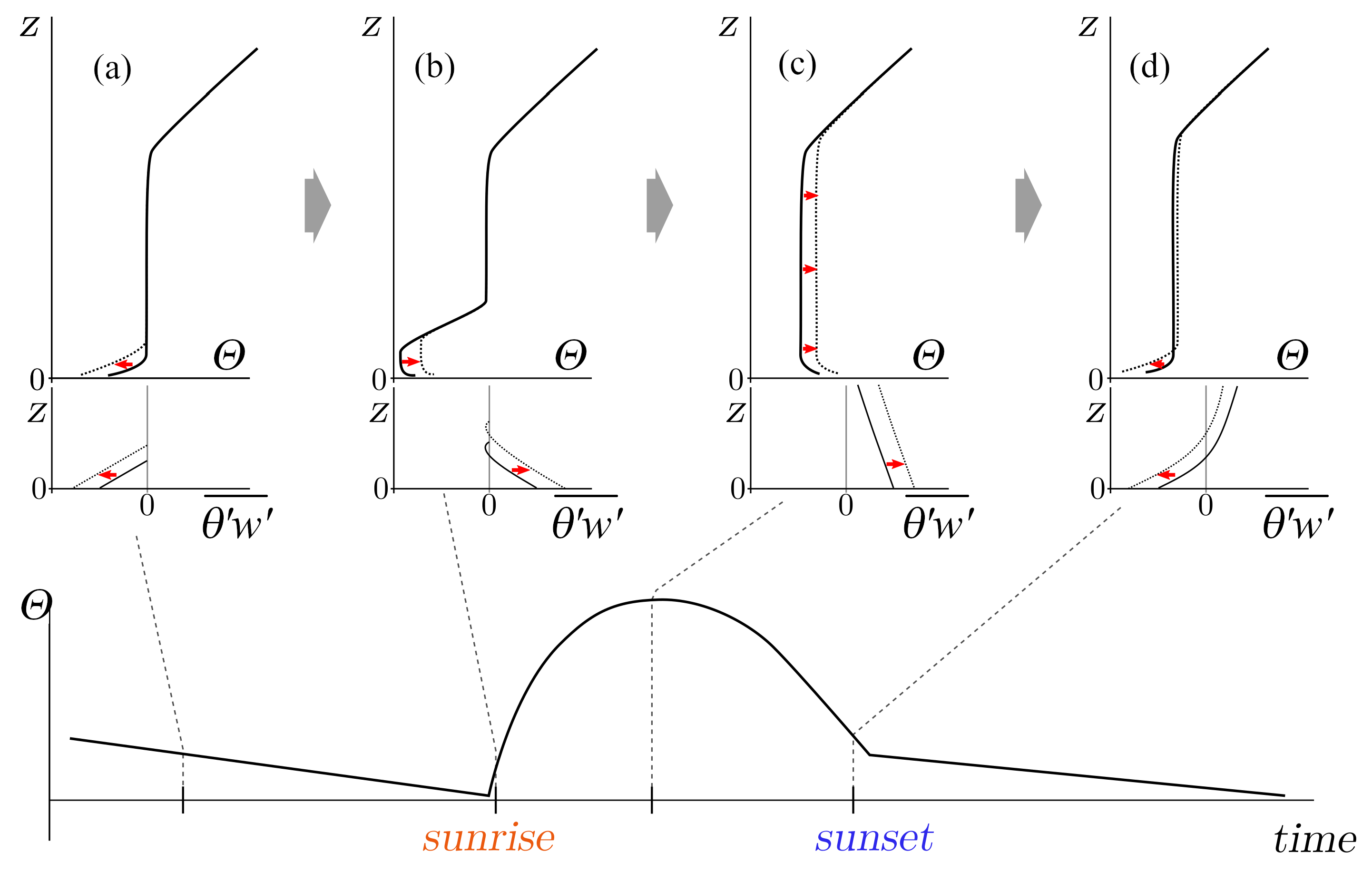
We start with the description of temperature profiles evolution during a typical diurnal cycle of dry ABL. The simplified picture of the profile evolution is presented in Figure 1.
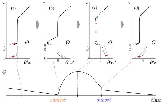
Figure 1.
A simplified schematics of the temperature profile evolution during the diurnal cycle in a dry ABL. (a) Nocturnal stable conditions. (b) Morning transition. (c) Daytime well-mixed conditions. (d) Evening transition.
We select three typical stages of the diurnal cycle. Firstly, we consider the night cooling with the formation of ground inversion. At this stage, sensible heat flux becomes negative (i.e., toward the ground). The growth of the inversion height is gradual and accompanied by a slow decrease of the ground temperature. Above the inversion, the temperature does not change significantly during this stage. Vertical integration of temperature profile from the ground up to the inversion height is proportional to the (negative) amount of heat lost during the cooling stage (Figure 1a).
Secondly, when the morning transition occurs, the mixed layer starts to grow from the ground with almost uniform bulk temperature profile (Figure 1b). The top of this mixed layer, as it progresses toward the higher temperatures, is following the “frozen” nocturnal temperature profile (ground inversion). When the heat accumulated during this stage becomes equal to the heat lost during the nocturnal cooling, a fast “jump” occurs of the the mixed layer height and it occupies the full volume below the long-term capping inversion at higher altitude (Figure 1c). Then, the profile evolves similarly to a typical penetrative convection. The heat from the ground is distributed over the whole height of the mixed layer, leading to its mean temperature growth.
Thirdly, at the time of evening transition when the sun heating weakens (Figure 1d) and the ground temperature drops below the bulk temperature of the mixed layer, a new ground inversion starts to grow and the cycle repeats.
In both situations of nocturnal cooling and daytime heating, the maximum of vertical turbulent heat flux is located near the surface. The turbulent heat flux decreases to zero when going up to the mixed or stratified layer height. In both cases, the simplest approximation for the heat flux profile is a linear function. With this simplification, it could be interpreted as the heat flux from the ground is distributed equally over the bulk of the stratified/mixed layer.
From the described above-described picture of the simplified evolution of temperature profile, it is clear that the single-cell model must take into account the heat accumulated in the near-ground layer to be able to reproduce more or less realistic sensible flux data.
For the simplified model construction, we will assume the following form of the near-ground profiles of temperature and velocity,
Their shapes are similar to standard wall-functions [37] parameterised by . Where is the near-ground turbulence kinetic energy, and are the near-ground turbulent heat and momentum fluxes, is ground temperature, and are thermal and momentum roughness scales.
We introduce the height of the near-ground layer (either stable or unstable depending on time) h and the temperature at the top of this level . These two last parameters are essential to fully specify the temperature profile. is assumed to change much slower, compared to the ground temperature during the whole diurnal cycle.
It is possible to integrate the heat flux vertically (up to h) to obtain the total accumulated heat per unit area (we will omit the multiplication by specific heat and density for simplicity):
Assuming that the roughness height is much lower then the total height of the layer, we can use the following approximation:
This equation can be inverted to obtain h given the accumulated heat Q, ground temperature and top temperature :
The accumulated heat can be computed by integration over time of the reconstructed ground heat flux:
In the cooling phase, the upper temperature is assumed to be constant but when the cooling stops and the bottom heat flux changes its sign, the mixed layer of penetrative convection starts to grow from the ground. Its growth is limited by the capping inversion created during the night (see Figure 1b).
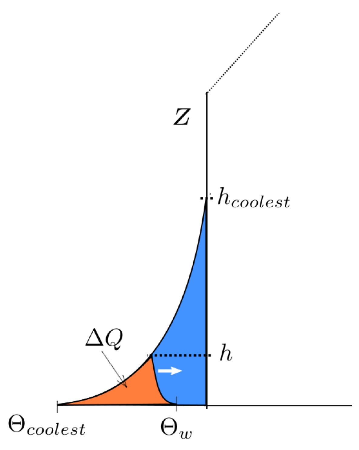
In Figure 2, the amount of heat accumulated during the morning transition () is shown graphically. It could be obtained by integration over the intersection of two logarithmic curves computed from Equation (21) with the same h. The first logarithmic curve is the coolest profile of the nocturnal cooling from the preceding night (which at the ground level has the temperature value ). The second curve (the current temperature profile) is inverted and has the value at the ground. Simple integration leads to the following estimate:
and

Figure 2.
Single-cell model schematics. Heating phase. Dotted line shows the height of a growing mixed layer. White arrow shows the direction of a daytime temperature profile evolution.
We store the last (coolest) profile of the cooling phase after the heat flux changes its sign. Then, for the heating stage, while , Q in Equation (25) should be replaced by . After the ground temperature in the heating phase becomes equal to the top temperature (Figure 1c), we return to the original formulations of Equation (25). In the evening transition, after the becomes less then the cycle repeats from the first phase.
The Reynolds stress value was calculated from Equation (20) assuming that value of velocity at some high altitude is remaining constant throughout the simulation. Based on the given velocity profiles from observation [14], this value was chosen to be 8 m s at an altitude of 800 m.
To close the system we need to solve the prognostic equation on :
where
Here, we use the standard turbulent viscosity relation (similar to (1)):
Finally, we obtained the dissipation value from integration over the non-dimensional height from 0 to 300:
The value 300 for was obtained by fitting with the observational data. It can be seen as the value of “effective” height of a surface layer that governs the near-ground turbulent fluxes.
2.3. Single-Column Formulation
In the Single-column mode, we consider the prognostic equations for temperature and two horizontal components of the flow velocity:
For the turbulence closure, we chose three variants, described above as Model 0, Model 1 and Model 2.
Wall Functions
For RANS simulations with coarse mesh, it is practical to use wall-functions approach for boundary conditions. In the current single-column simulations, we use the following wall-functions formulation. Assuming the log law for temperature and velocity profiles, we obtain [37]:
where and are the values of temperature and horizontal velocity in the first grid node, at the altitude of .
Making the heat flux in the first grid node equal to the wall heat flux, we obtain the following boundary condition for potential temperature:
Similarly, for the velocity in the first grid point we obtain:
where for brevity:
For k zero-gradient condition is chosen for the bottom boundary. The energy dissipation rate at the first grid node was set to its standard value:
This concludes the model description. One important addition is the estimate of boundary layer height h. To estimate this quantity, we used the assumption of linear height dependence of the turbulent heat flux. We assume that turbulent heat flux decays to zero linearly from the bottom where its magnitude is maximal to the top of the boundary layer. With this, we use the following relation to estimate the value of h from the near-surface data:
The obtained value of h 10–850 m. This value was used as in Model 3.
2.4. Initial and Boundary Conditions and Numerical Details
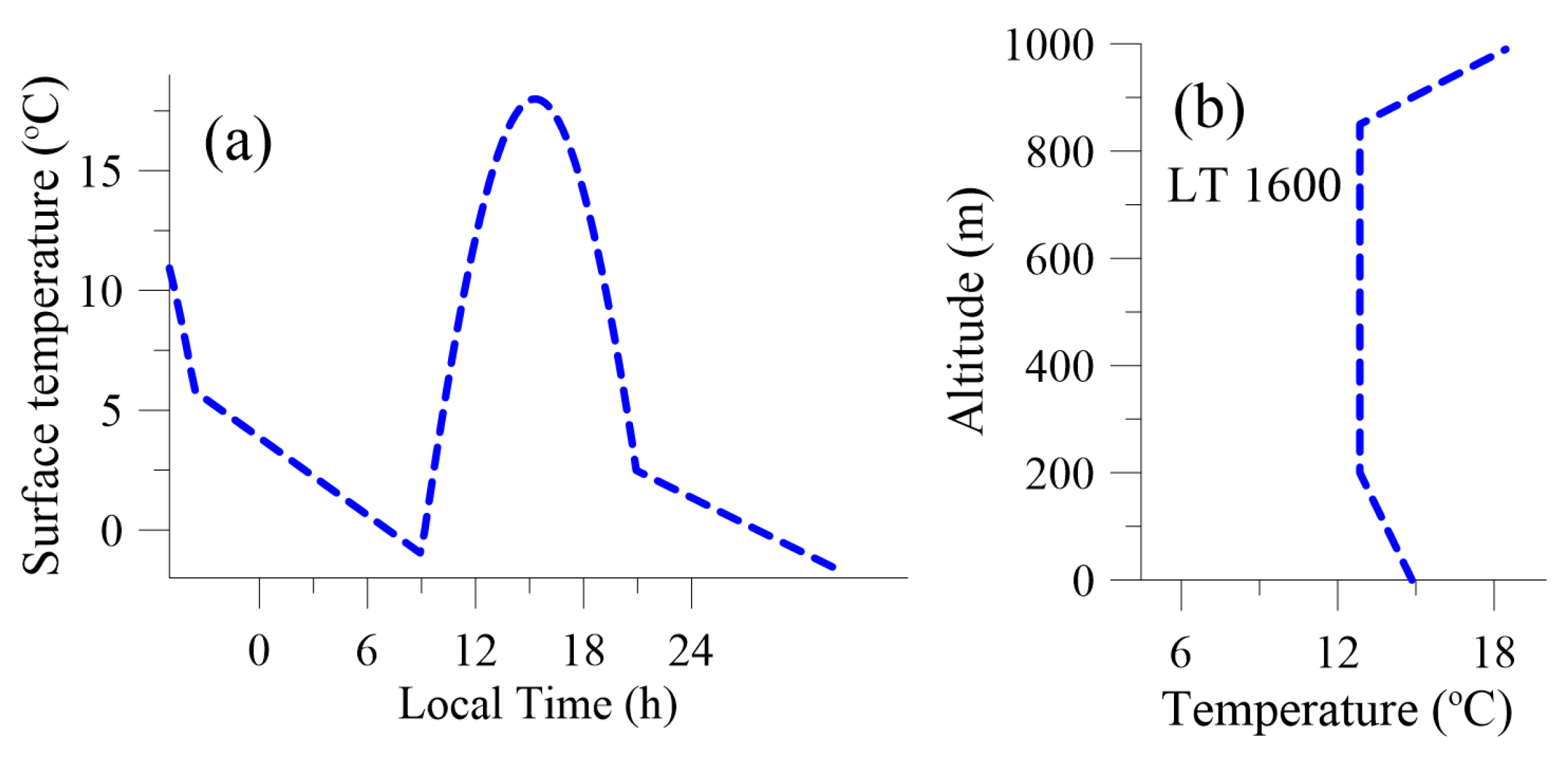
The parameters of the simulations were taken similarly to those recommended in GABLS2 [14] intercomparison. The following values for case-specific constants were used: m , m , , m, m. As recommended in [14], the simulation starts at LT 1600 of 22 October data point for 48 h. The initial temperature profile and the surface temperature evolution plot are shown in Figure 3. For k and , the initial uniform profiles were set with values 0.01 and 0.001 respectively. For single-column simulations, a uniform grid was used with a cell height of 6 m (three more grids with cell heights of 1.5 m, 3 m and 12 m were also tested). The total grid height was 4000 m. At the top boundary, constant gradient condition of C/km was set for potential temperature. For all other prognostic variables, zero gradient conditions were set at the top boundary. The time step of the simulation was set to 0.02 s. The first order Euler scheme was used for the discretization of time derivative. The prognostic variables were calculated at the grid nodes, while the turbulent fluxes were calculated at the midpoints between the adjacent nodes, thus creating a staggered grid. The central differencing scheme was used for the spatial derivative discretization. The diffusion term is discretized in the following way:
where is prognostic variable, is the effective diffusivity, n is the current iteration number. The quantities indexed with n are treated by implicit scheme. Index marks the values taken from previous iteration (via deferred correction). The index i corresponds to the grid node number. The sweep of several iterations per time step was used until the mutual convergence of all residuals. Iterations were done over all prognostic variables.
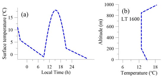
Figure 3.
(a) Surface temperature time plot (data taken from [14]). (b) Initial temperature profile (assigned to 16:00 local time).
3. Simulation Results
The data from GABLS2 contains both stable and unstable flow regimes with morning and evening transitions. This allows not only checking the equilibrium states prediction by single-column models but also the dynamic transitional effects.
As reported in [14], the correct description of the morning transition was one of the most problematic part for the majority of compared models. Another important point is the correct energy balance (both thermal and kinetic) during the diurnal cycle as it affects the overall evolution of the boundary layer. This balance is dependent on the correct reconstruction of surface fluxes.
In this section, we present the results of testing the proposed modification of the model in two aspects: the dynamics of transition and surface fluxes reconstruction, together with the results of alternative formulations.
3.1. Single-Cell Model
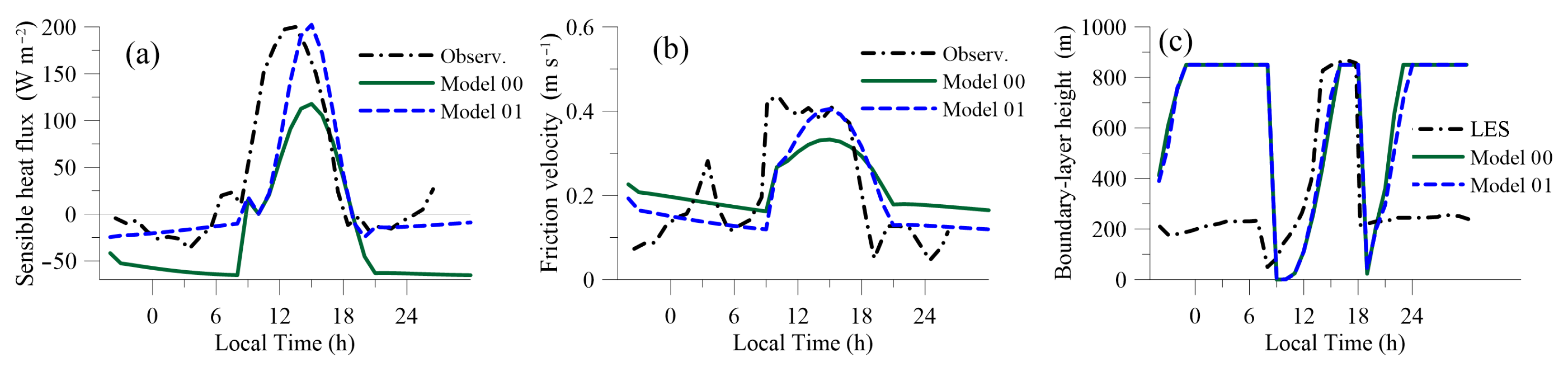
We compare the reconstructed fluxes with the observed data for two single-cell model formulations: one with standard form of the k equation (Model 00), and the other with the proposed modification (Model 01, Equations (28) and (29)). Figure 4a shows the comparison of the observed and reconstructed sensible heat flux evolution. It can be seen that during the nighttime the difference between the models is significant. Model 00 shows much higher magnitude of the negative sensible heat flux overpredicting the observed value. This behaviour was observed for many models from [14] in the nighttime (including LES simulation).
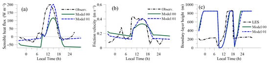
Figure 4.
Comparison of single-cell results with observations data from [14]. (a) Sensible heat flux evolution. (b) Friction velocity evolution. (c) Boundary-layer height evolution compared with LES from [14].
The presented modification of the Reynolds stress (Model 01) improves this behaviour, making the heat flux very close to the observed values in the nighttime. For the friction velocity (Figure 4b), both models give close results in the nighttime, with Model 01 being slightly lower. While it is hard to say definitely which model gives better prediction for morning part of the simulation, for the evening stability conditions Model 01 is closer to the observations.
In the daytime, the picture inverses and Model 01 shows higher magnitudes of sensible heat flux and friction velocity then Model 00. Both the heat flux and friction velocity show much improved values with the proposed buoyancy-induced modification. The peak night time and daytime sensible heat fluxes are reconstructed quite well with the proposed single-cell model.
However, both models show a significant lag in the onset of morning transition. This was also noted for many models tested in GABLS2. We speculate that this is a consequence of the inability of the models to account for the growth of coherent convective cells that accelerate mixing during the morning transition.
Due to their simplicity, single cell models give unrealistic results for the boundary-layer height (Figure 4c). Especially in the nighttime, the models show unrealistically high values of h (obtained from Equation(24). However, during the daytime, the growth rate of h is quite realistic, resembling the LES result but again with some temporal lag.
In general, the proposed form of a single-cell model gives good results for surface fluxes reconstruction, which make it attractive for further development as a wall-function model for complex 3D ABL simulations.
3.2. Single Column Model
3.2.1. Numerical Resolution Effects
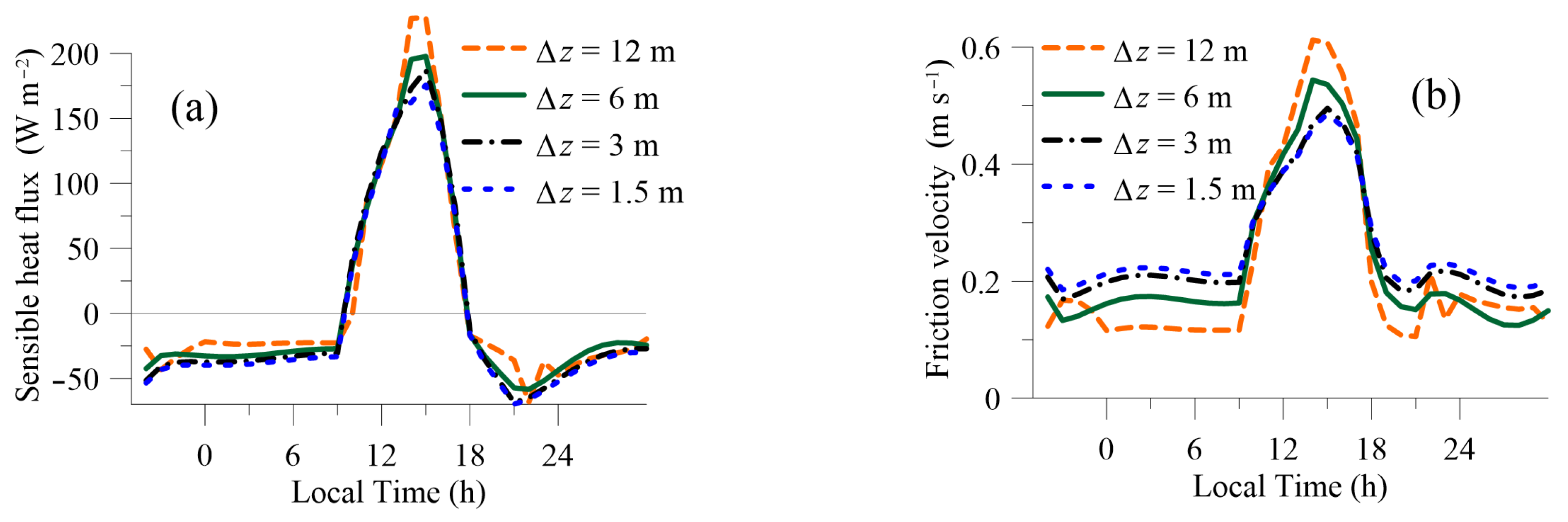
We start the discussion of single-column results by checking the grid dependence of the solution. In GABLS2 [14], noticeable difference between the results with near wall grid step of less than 5 m and more than 5 m was reported. For the current model we checked four resolutions: 1.5 m, 3 m, 6 m and 12 m. The results are shown in Figure 5.

Figure 5.
The results of grid sensitivity test of Model 1: (a) Sensible heat flux. (b) Friction velocity.
It can be seen that the results converge for the grid resolution of 1.5 m. For grid steps of 1.5, 3 and 6 m, all the heat flux plots are very close, while for 12 m we see some small difference in the daytime. Still, even for such coarse resolution (12 m), sensible heat flux shows almost grid-independent results and the friction velocity is changed mildly with increasing the resolution several times.
This change with grid coarsening is expected because the gradients become less and less resolved. However, as the model assumes well-developed logarithmic layer for both temperature and velocity at the first grid node, the height of the first grid node in wall units should be at least >100. In our case, have shown the best agreement with the experiments, which corresponds to m. The below-reported results were obtained with the uniform grid spacing of = 6 m. We consider this a practical resolution for a 3D computational RANS code where the proposed model can be used.
3.2.2. Stable Regime
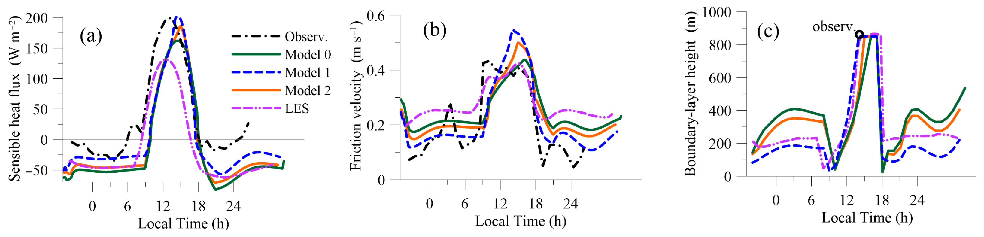
From the comparison of the considered models with in situ observations (Figure 6a), it can be seen that before the morning transition all three models underestimate the sensible heat flux. The same underestimation is also observed for 3D LES results from [14]. However, Model 1 shows lower magnitude of negative heat flux than two other Models (and LES results). Model 2, which utilises a modified definition (11) of turbulent viscosity, shows very little difference from the standard (Model 0) in terms of sensible heat flux magnitude, thus illustrating the effect of compensation, described in Section 2.1.2.
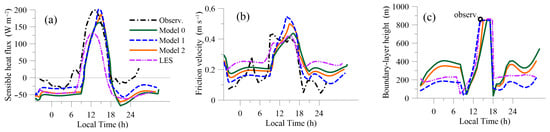
Figure 6.
Comparison of single-column results with observations data from [14]. (a) Sensible heat flux evolution. (b) Friction velocity evolution. (c) Boundary-layer height evolution. LES data taken from [14].
The proposed modification (Model 1) is significantly more sensitive to the stability effects.
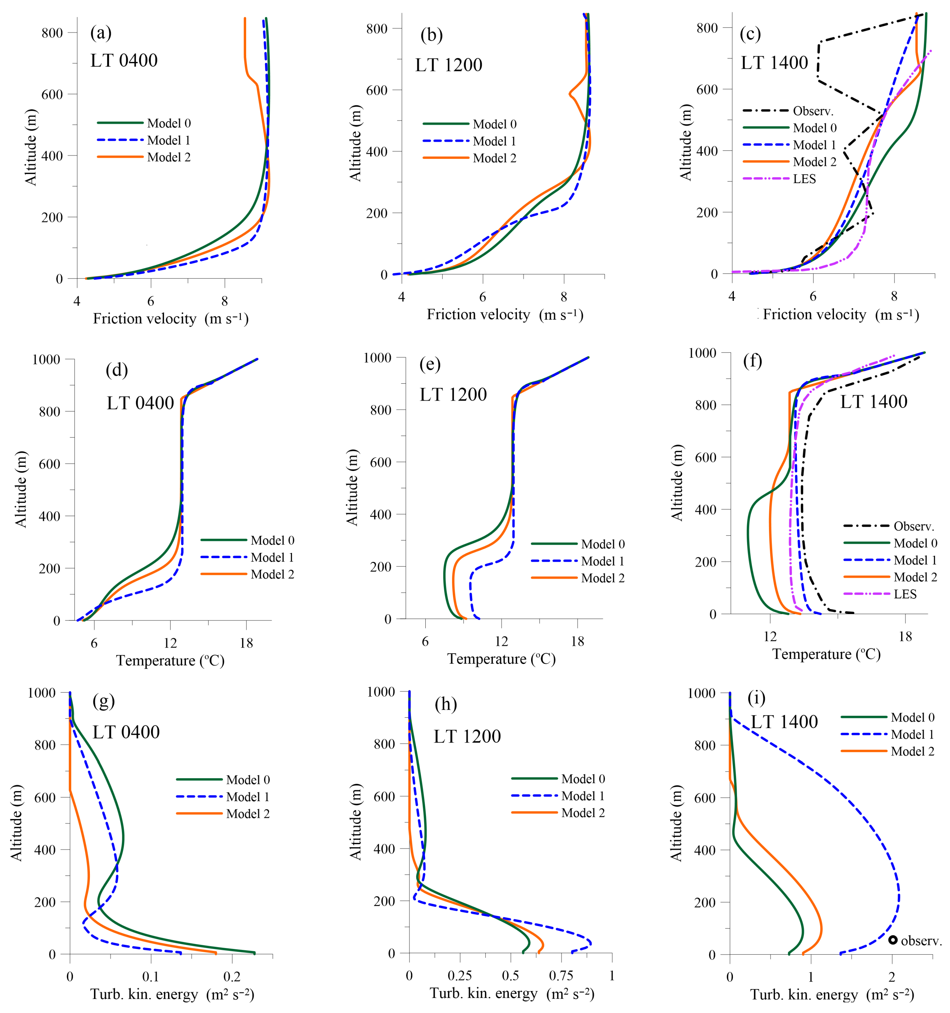
In the temperature profiles in Figure 7d, this is also evident as the boundary layer height is lower for Model 1 due to less heat lost during the nighttime.
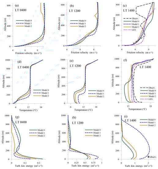
Figure 7.
Vertical profiles of flow variables at different time instants: (a–c) Wind speed. (d–f) Potential temperature. (g–i) Turbulence kinetic energy. Black circle with in subplot (i) corresponds to a measured TKE value reported in [14].
For friction velocity (Figure 7b), Model 1 shows the lowest values in the nighttime and is in better agreement with observations in comparison with two other Models and 3D LES results from [14].
The evolution of the boundary-layer height h shows (Figure 6c) that Model 0 and Model 2 noticeably overpredict the value of h in the nighttime (Model 2 being a little closer to the LES values) while Model 1 is in a much better agreement with the data from [14].
The vertical profiles of velocity for nocturnal conditions are shown in Figure 7a. It can be seen that Model 2 here forms an overshoot (nocturnal low jet) in the upper part of boundary layer, while the other two Models do not. Such behaviour is in agreement with the observations and shows a positive effect of limiting the mixing length. The Model 0 and the proposed Model 1 do not show this behaviour. However, the velocity profile for Model 2 also shows an overestimation of the ABL height, while Model 1 gives more realistic results for this parameter.
The effect of limiting of the mixing length in Model 2 is also evident in the distribution of turbulence kinetic energy (Figure 7g). The two-peak structure of TKE is seen in Model 1 and Model 0 results, while this second peak at higher altitude is almost absent in Model 2. This behaviour is in a better agreement with MOST. However, the values of TKE near the ground are closer to the observations in Model 1.
3.3. Morning Transition and Daytime Unstable Conditions
During the morning transition, the observed height of the ABL grows rapidly. This is accompanied by the increase in wall shear stress and wind speed. The morning transition has its effects on heat and momentum fluxes. From Figure 6a, it can be seen that Model 1 predicts heat flux peak magnitude quite well but shows a delay in the transition time similarly to the single-cell case. The other two Models also show that delay, while 3D LES capture the transition moment quite accurately. Model 1 shows the values of the peak daytime heat flux closest to the observations, while other two Models and LES underpredict it.
From the vertical plots of temperature (Figure 7e,f), it is clear that Model 1 reproduce the thermal energy balance of the flow more correctly than other two Models. Comparison with the observed temperature profile at LT 1400 in Figure 7f showed significantly lower temperatures and different phase of ABL evolution for Models 0 and 2. Model 1 shows results much closer to the observations. This is the consequence of overestimation of negative sensible heat flux during the night in Models 0 and 2.
The friction velocity behaviour (Figure 6b) is similar to many models reported in [14] and it shows a gradual growth instead of a rapid transition observed experimentally. This deviation from the observed values might be due to the lack of contribution of the coherent structures (convective cells and rolls) to the heat and momentum flux values. These structures are resolved in 3D LES, which is reflected in a good agreement of daytime 3D LES data with observations. For the proposed model, this issue might be improved with a transition to 3D simulations. The value of friction velocity produced by Model 1 is slightly overestimated in the later part of the day compared to the results of two other models, but the slope of the growth of friction velocity is higher, showing a faster transition dynamics than the other two Models.
For the wind speed profiles (Figure 7b,c), Model 2 gives a more physically correct shape of the profiles, while Model 1 gives more correct predictions of the boundary-layer height. This is evident in comparison with experimentally observed wind speed profile at LT 1400 (Figure 7c).
This faster transition is also evident in the plot of boundary-layer height dynamics (Figure 6c). Model 1 has the fastest growth of h, close to the LES results from [14]. Here again, Model 2 is showing the results between Model 0 and Model 1.
3.4. Evening Transition
During the evening transition, the model and some first-order models from [14] show a negative peak of sensible heat flux also visible in all single-column results of the current paper (Figure 6a) at LT2100. A similar negative peak but of more diffuse shape is seen even in the 3D LES results from [14]. However, it is absent in the field observations. We speculate that the probable reason for that is a violation of the gradient diffusion hypothesis at this moment on which all and LES models are based. This effect also pronounced in recent GABLS4 [7] intercomparison where the majority of LES models overestimate the magnitude of negative sensible heat flux during the transition to stability. This effect needs further investigation as it plays an important part in the thermal energy balance of the diurnal cycle.
Among the models tested in this paper, the lowest amplitude of this effect is in Model 1. Model 0 and Model 2 show quite similar behaviour. The h evolution during the transition to stability shows also much better results for Model 1 (Figure 6c).
4. Conclusions
A modification of a standard model is presented with possible applications to the diurnal cycle simulations of dry ABL. The modification accounts for buoyancy effects using local Richardson number as a parameter for intensification/damping of vertical momentum and heat fluxes. The model is tested on atmospheric observation data and showed better restoration capability of sensible heat and momentum fluxes compared to the standard model and its scale-limited modification.
In comparison to other buoyancy-adjusted modifications, our model shows higher sensitivity to the local stability conditions due to a lack of compensation effects on turbulent viscosity.
The presented form of Reynolds stress and turbulent heat flux parametrizations modification that also satisfies the equilibrium conditions in buoyancy affected cases is free from this compensation effects and thus is more sensitive to the stability variations. All the model constants of the original model remain their values, so the proposed stability adjustment could be easily implemented for complex 3D simulations.
The proposed simplified single-cell approach is promising concerning the development of new stability-adjusted wall-functions for a more correct representation of sensible heat and momentum fluxes.
Author Contributions
Conceptualization, methodology, M.H.; software, validation, M.B.; formal analysis, M.H. and M.B.; writing—original draft preparation, M.H. and M.B.; writing—review and editing, M.H.; visualization, M.B. All authors have read and agreed to the published version of the manuscript.
Funding
The study was supported by the Ministry of Science and Higher Education of the Russian Federation (agreement No. 075-15-2020-806).
Institutional Review Board Statement
Not applicable.
Informed Consent Statement
Not applicable.
Data Availability Statement
Not applicable.
Conflicts of Interest
The authors declare no conflict of interest.
Abbreviations
The following abbreviations are used in this manuscript:
| ABL | Atmospheric Boundary Layer |
| RANS | Reynolds-Averaged Navier Stokes |
| LES | Large Eddy Simulation |
| TKE | Turbulence Kinetic Energy |
| CASES-99 | Cooperative Atmospheric Surface Exchange Study |
| GABLS | GEWEX Atmospheric Boundary Layer Study |
References
- Monin, A. The atmospheric boundary layer. Annu. Rev. Fluid Mech. 1970, 2, 225–250. [Google Scholar] [CrossRef]
- Kaimal, J.C.; Finnigan, J.J. Atmospheric Boundary Layer Flows: Their Structure and Measurement; Oxford University Press: Oxford, UK, 1994. [Google Scholar]
- Garratt, J.R. The atmospheric boundary layer. Earth-Sci. Rev. 1994, 37, 89–134. [Google Scholar] [CrossRef]
- Monin, A.; Obukhov, A. Basic laws of turbulent mixing in the atmosphere near the ground. Tr. Geofiz. Inst. Akad. Nauk SSSR 1954, 24, 163–187. [Google Scholar]
- Stoll, R.; Gibbs, J.A.; Salesky, S.T.; Anderson, W.; Calaf, M. Large-eddy simulation of the atmospheric boundary layer. Bound.-Layer Meteorol. 2020, 177, 541–581. [Google Scholar] [CrossRef]
- Van Heerwaarden, C.C.; Mellado, J.P.; De Lozar, A. Scaling laws for the heterogeneously heated free convective boundary layer. J. Atmos. Sci. 2014, 71, 3975–4000. [Google Scholar] [CrossRef]
- Couvreux, F.; Bazile, E.; Rodier, Q.; Maronga, B.; Matheou, G.; Chinita, M.J.; Edwards, J.; van Stratum, B.J.; van Heerwaarden, C.C.; Huang, J.; et al. Intercomparison of large-eddy simulations of the Antarctic boundary layer for very stable stratification. Bound.-Layer Meteorol. 2020, 176, 369–400. [Google Scholar] [CrossRef]
- Van Stratum, B.J. The Influence of Misrepresenting the Nocturnal Boundary Layer on Daytime Convection in Large-Eddy Simulation. Ph.D. Thesis, Universität Hamburg, Hamburg, Germany, 2017. [Google Scholar]
- Hanjalić, K.; Launder, B.E. A Reynolds stress model of turbulence and its application to thin shear flows. J. Fluid Mech. 1972, 52, 609–638. [Google Scholar] [CrossRef]
- Mellor, G.L.; Yamada, T. A hierarchy of turbulence closure models for planetary boundary layers. J. Atmos. Sci. 1974, 31, 1791–1806. [Google Scholar] [CrossRef] [Green Version]
- André, J.; De Moor, G.; Lacarrere, P.; Du Vachat, R. Modeling the 24-hour evolution of the mean and turbulent structures of the planetary boundary layer. J. Atmos. Sci. 1978, 35, 1861–1883. [Google Scholar] [CrossRef] [Green Version]
- Canuto, V.; Minotti, F.; Ronchi, C.; Ypma, R.; Zeman, O. Second-order closure PBL model with new third-order moments: Comparison with LES data. J. Atmos. Sci. 1994, 51, 1605–1618. [Google Scholar] [CrossRef]
- Ilyushin, B. Simulation of the diurnal evolution of the atmospheric boundary layer. Izv. Atmos. Ocean. Phys. 2014, 50, 246–255. [Google Scholar] [CrossRef]
- Svensson, G.; Holtslag, A.; Kumar, V.; Mauritsen, T.; Steeneveld, G.; Angevine, W.; Bazile, E.; Beljaars, A.; De Bruijn, E.; Cheng, A.; et al. Evaluation of the diurnal cycle in the atmospheric boundary layer over land as represented by a variety of single-column models: The second GABLS experiment. Bound.-Layer Meteorol. 2011, 140, 177–206. [Google Scholar] [CrossRef] [Green Version]
- Zhang, D.L.; Zheng, W.Z. Diurnal cycles of surface winds and temperatures as simulated by five boundary layer parameterizations. J. Appl. Meteorol. Climatol. 2004, 43, 157–169. [Google Scholar] [CrossRef] [Green Version]
- Tjernström, M.; Žagar, M.; Svensson, G.; Cassano, J.J.; Pfeifer, S.; Rinke, A.; Wyser, K.; Dethloff, K.; Jones, C.; Semmler, T.; et al. Modelling the Arctic boundary layer: An evaluation of six ARCMIP regional-scale models using data from the SHEBA project. Bound.-Layer Meteorol. 2005, 117, 337–381. [Google Scholar] [CrossRef]
- Steeneveld, G.; Mauritsen, T.; De Bruijn, E.; Vilà-Guerau de Arellano, J.; Svensson, G.; Holtslag, A. Evaluation of limited-area models for the representation of the diurnal cycle and contrasting nights in CASES-99. J. Appl. Meteorol. Climatol. 2008, 47, 869–887. [Google Scholar] [CrossRef]
- Antoon van Hooft, J.; Baas, P.; van Tiggelen, M.; Ansorge, C.; van de Wiel, B.J. An idealized description for the diurnal cycle of the dry atmospheric boundary layer. J. Atmos. Sci. 2019, 76, 3717–3736. [Google Scholar] [CrossRef]
- Apsley, D.D.; Castro, I.P. A limited-length-scale k-ε model for the neutral and stably-stratified atmospheric boundary layer. Bound.-Layer Meteorol. 1997, 83, 75–98. [Google Scholar] [CrossRef]
- Freedman, F.R.; Jacobson, M.Z. Modification Of The Standard∈-Equation For The Stable Abl Through Enforced Consistency With Monin–Obukhov Similarity Theory. Bound.-Layer Meteorol. 2003, 106, 383–410. [Google Scholar] [CrossRef]
- Kurbatskiy, A.F.; Kurbatskaya, L.I. E − ε − <θ 2> turbulence closure model for an atmospheric boundary layer including the urban canopy. Meteorol. Atmos. Phys. 2009, 104, 63–81. [Google Scholar]
- Sumner, J.; Masson, C. The Apsley and Castro Limited-Length-Scale Model Revisited for Improved Performance in the Atmospheric Surface Layer. Bound.-Layer Meteorol. 2012, 144, 199–215. [Google Scholar] [CrossRef]
- Hanjalić, K.; Hrebtov, M. Ground boundary conditions for thermal convection over horizontal surfaces at high rayleigh numbers. Bound.-Layer Meteorol. 2016, 160, 41–61. [Google Scholar] [CrossRef]
- Kenjeres, S.; Hanjalic, K. Combined effects of terrain orography and thermal stratification on pollutant dispersion in a town valley: A T-RANS simulation. J. Turbul. 2002, 3, 026. [Google Scholar] [CrossRef]
- Kenjereš, S.; Hanjalić, K. LES, T-RANS and hybrid simulations of thermal convection at high Ra numbers. Int. J. Heat Fluid Flow 2006, 27, 800–810. [Google Scholar] [CrossRef]
- Hrebtov, M.; Hanjalić, K. Numerical study of winter diurnal convection over the city of Krasnoyarsk: Effects of non-freezing river, undulating fog and steam devils. Bound.-Layer Meteorol. 2017, 163, 469–495. [Google Scholar] [CrossRef]
- Hrebtov, M.; Hanjalić, K. River-induced anomalies in seasonal variation of traffic-emitted CO distribution over the City of Krasnoyarsk. Atmosphere 2019, 10, 407. [Google Scholar] [CrossRef] [Green Version]
- Wilcox, D.C. Multiscale model for turbulent flows. AIAA J. 1988, 26, 1311–1320. [Google Scholar] [CrossRef]
- Jones, W.; Launder, B.E. The prediction of laminarization with a two-equation model of turbulence. Int. J. Heat Mass Transf. 1972, 15, 301–314. [Google Scholar] [CrossRef]
- Menter, F.R. Two-equation eddy-viscosity turbulence models for engineering applications. AIAA J. 1994, 32, 1598–1605. [Google Scholar] [CrossRef] [Green Version]
- Iaccarino, G.; Mishra, A.A.; Ghili, S. Eigenspace perturbations for uncertainty estimation of single-point turbulence closures. Phys. Rev. Fluids 2017, 2, 024605. [Google Scholar] [CrossRef]
- Mishra, A.A.; Duraisamy, K.; Iaccarino, G. Estimating uncertainty in homogeneous turbulence evolution due to coarse-graining. Phys. Fluids 2019, 31, 025106. [Google Scholar] [CrossRef]
- Poulos, G.S.; Blumen, W.; Fritts, D.C.; Lundquist, J.K.; Sun, J.; Burns, S.P.; Nappo, C.; Banta, R.; Newsom, R.; Cuxart, J.; et al. CASES-99: A comprehensive investigation of the stable nocturnal boundary layer. Bull. Am. Meteorol. Soc. 2002, 83, 555–582. [Google Scholar] [CrossRef]
- Yamada, T. The critical Richardson number and the ratio of the eddy transport coefficients obtained from a turbulence closure model. J. Atmos. Sci. 1975, 32, 926–933. [Google Scholar] [CrossRef]
- Zilitinkevich, S.; Elperin, T.; Kleeorin, N.; Rogachevskii, I.; Esau, I.; Mauritsen, T.; Miles, M. Turbulence energetics in stably stratified geophysical flows: Strong and weak mixing regimes. Q. J. R. Meteorol. Soc. J. Atmos. Sci. Appl. Meteorol. Phys. Oceanogr. 2008, 134, 793–799. [Google Scholar] [CrossRef] [Green Version]
- Freire, L.S.; Chamecki, M.; Bou-Zeid, E.; Dias, N.L. Critical flux Richardson number for Kolmogorov turbulence enabled by TKE transport. Q. J. R. Meteorol. Soc. 2019, 145, 1551–1558. [Google Scholar] [CrossRef]
- Launder, B.E.; Spalding, D.B. The numerical computation of turbulent flows. In Numerical Prediction of Flow, Heat Transfer, Turbulence and Combustion; Elsevier: Amsterdam, The Netherlands, 1983; pp. 96–116. [Google Scholar]
Publisher’s Note: MDPI stays neutral with regard to jurisdictional claims in published maps and institutional affiliations. |
© 2022 by the authors. Licensee MDPI, Basel, Switzerland. This article is an open access article distributed under the terms and conditions of the Creative Commons Attribution (CC BY) license (https://creativecommons.org/licenses/by/4.0/).