
Prediction Model of Carbon Dioxide Concentration in Pig House Based on Deep Learning

 ,
,  ,
,  and
and 
Abstract
:1. Introduction
2. Materials and Methods
2.1. Data Collection
2.2. Data Preprocessing
2.2.1. Data Interpolation
2.2.2. Data Normalization
2.3. Prediction Model of CO2 Concentration
2.3.1. BP Model
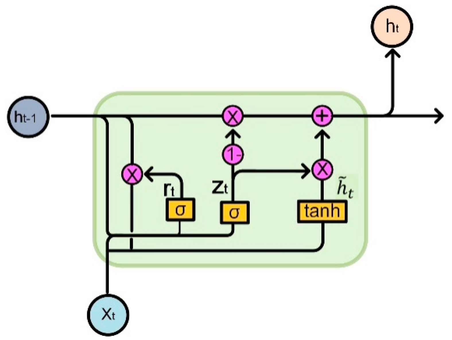
2.3.2. GRU Model
2.3.3. EMD
2.3.4. EEMD
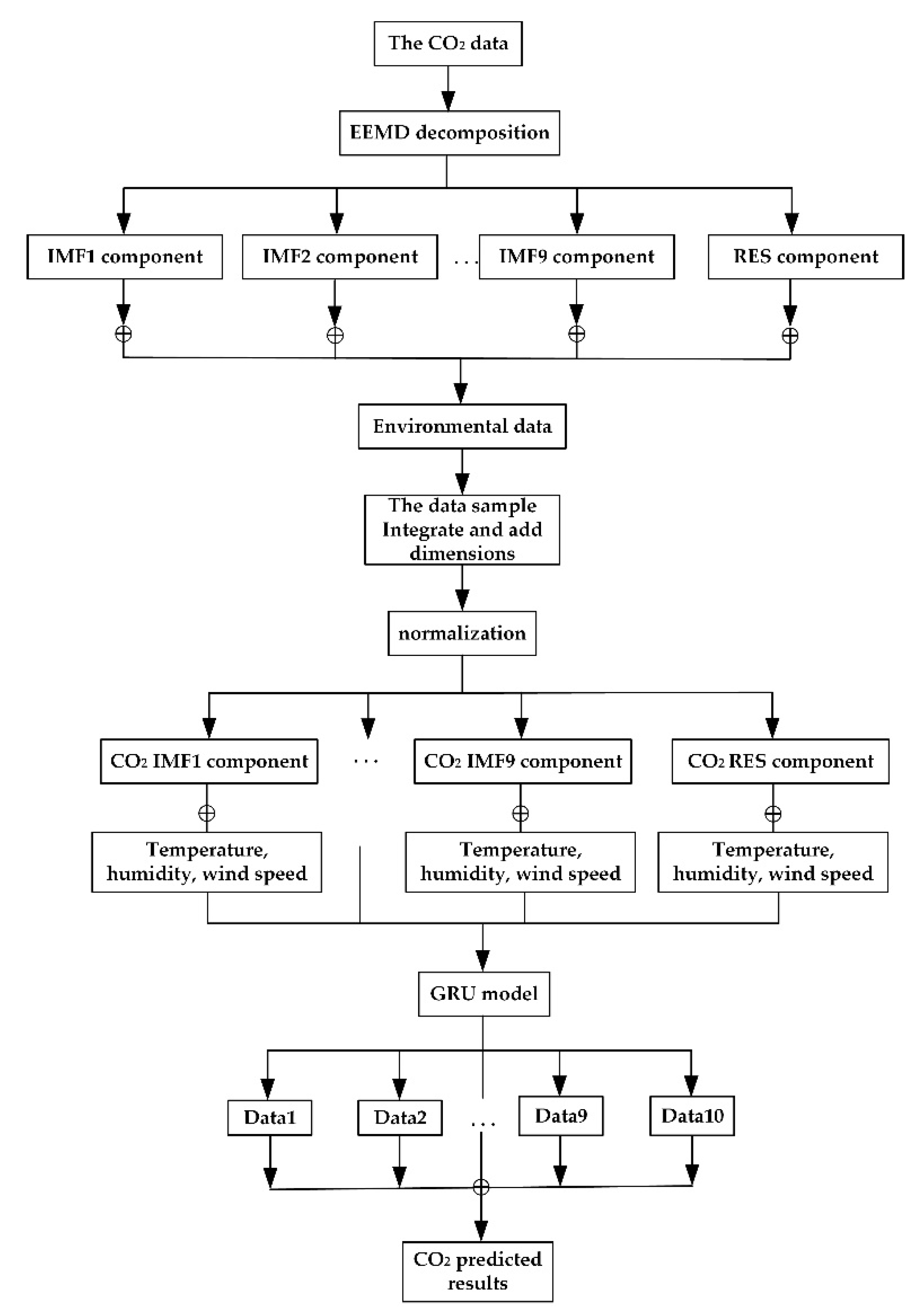
2.3.5. EEMD–GRU
2.4. Model Parameter Settings
2.5. Model Evaluation Index
3. Results and Discussion
3.1. Results and Analysis
3.1.1. Decomposition Result of EEMD
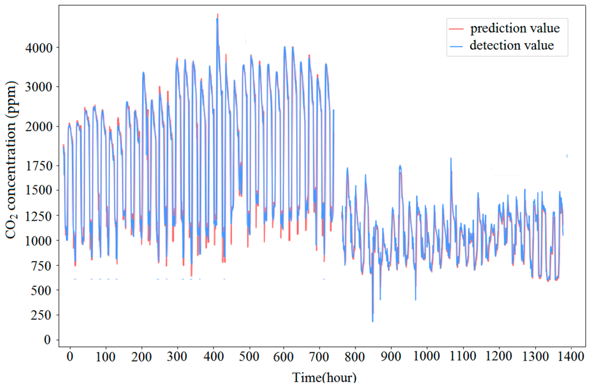
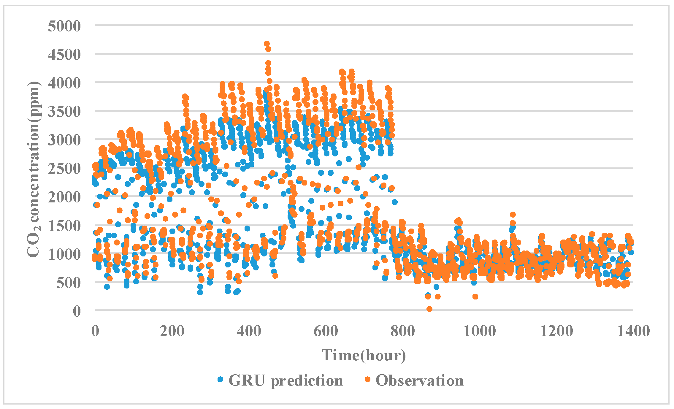
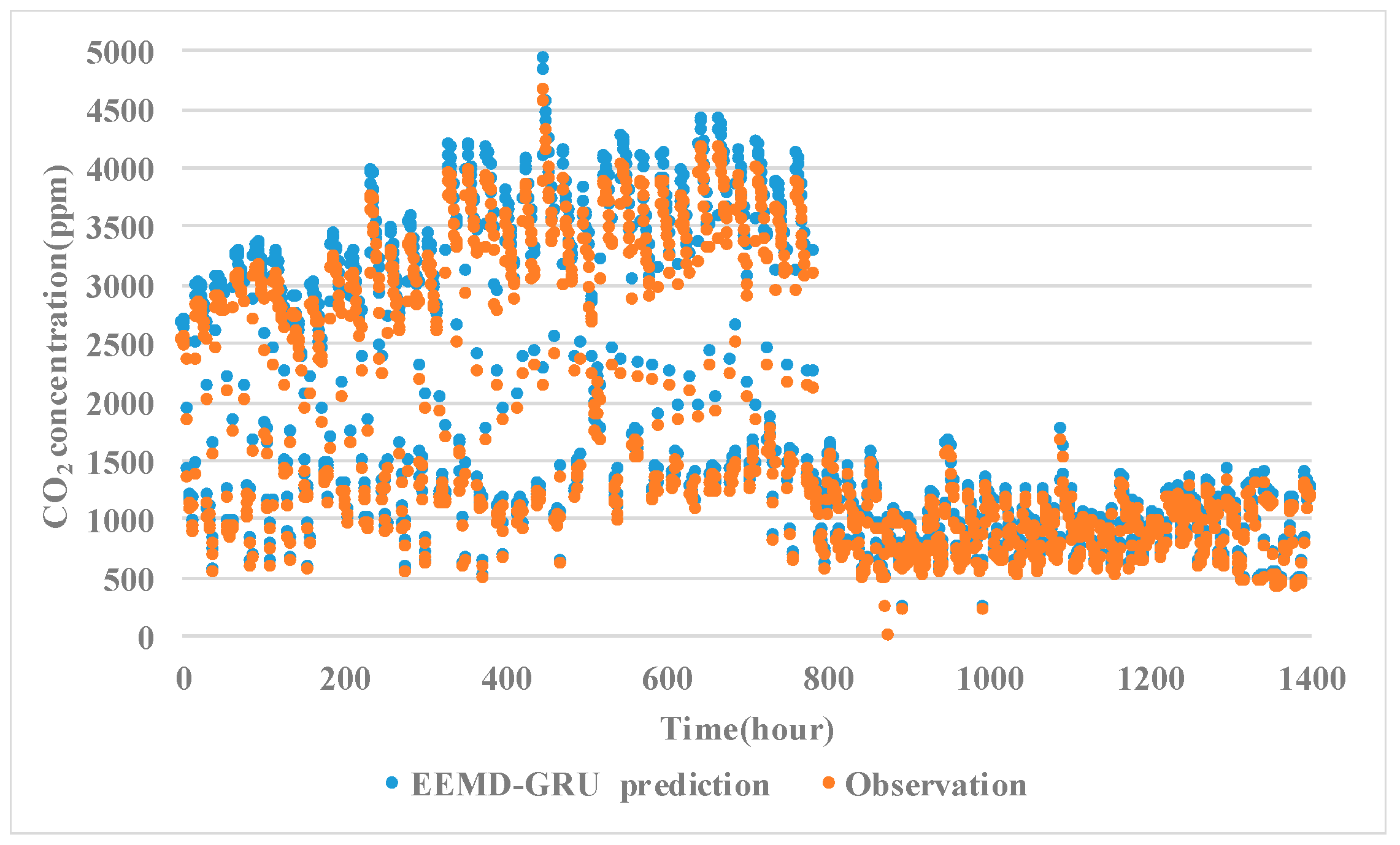
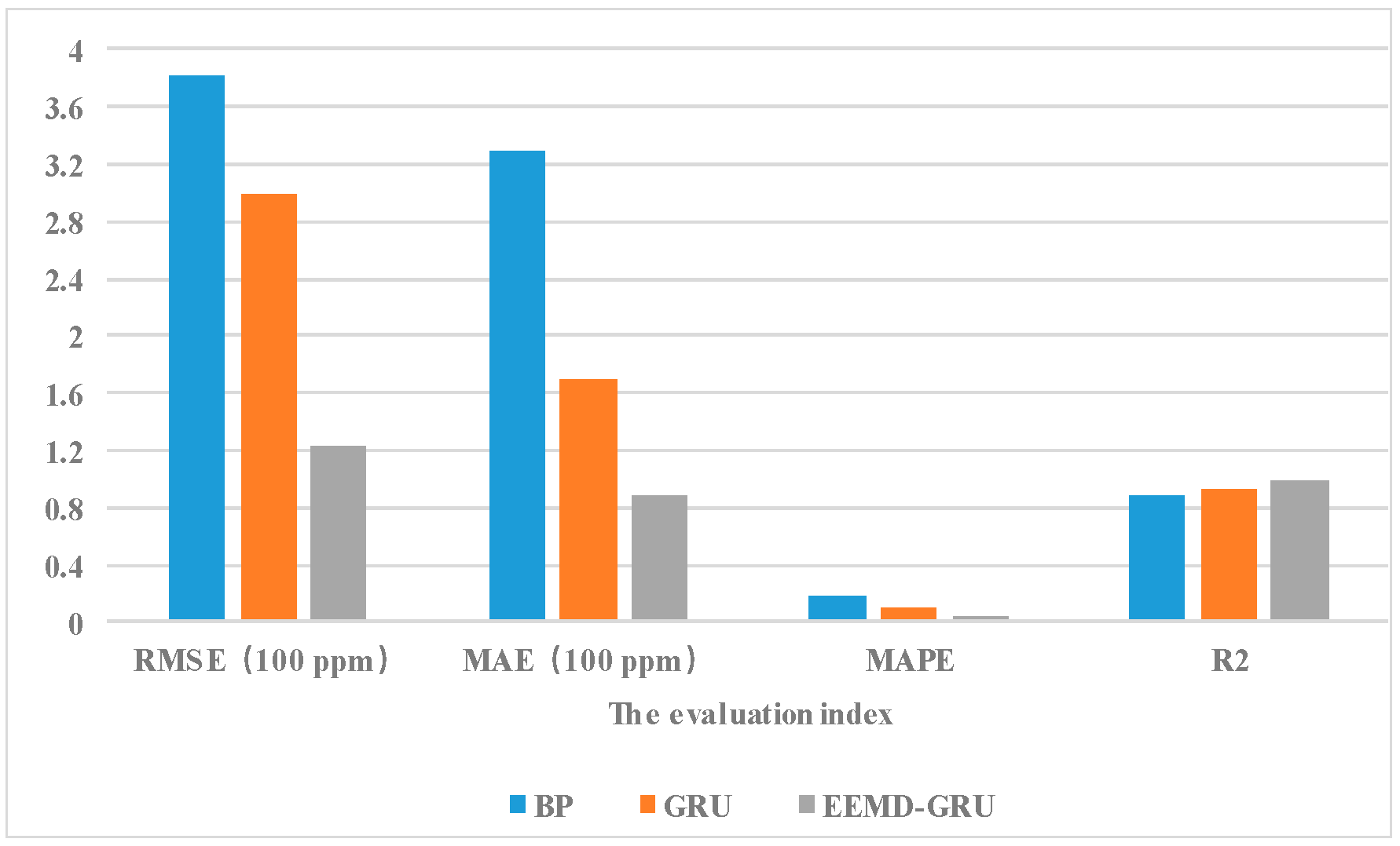
3.1.2. Results of Model Prediction
3.2. Discussion
4. Conclusions
Author Contributions
Funding
Institutional Review Board Statement
Informed Consent Statement
Data Availability Statement
Acknowledgments
Conflicts of Interest
References
- Liu, H.; Chen, Y. Development status, future development trend and suggestions of pig industry in 2021. Chin. J. Anim. Sci. 2022, 58, 204–209. [Google Scholar]
- Chen, J.; Feng, T.; Huang, S.; Hao, W.; Huo, J.; Zhu, W. Research on recognition of piggery environmental status based on D-S evidence theory. J. Chin. Agric. Mech. 2021, 42, 50–54. [Google Scholar]
- Wang, P.; Wang, C.; Xuan, C.; Ji, B.; Zong, Z. Research status of the detection and control methods of harmful gases in pig houses. Heilongjiang Anim. Sci. Vet. Med. 2017, 521, 53–57, 292. [Google Scholar]
- Guo, L.; Zhao, B.; Jia, Y.; He, F.; Chen, W. Mitigation Strategies of Air Pollutants for Mechanical Ventilated Livestock and Poultry Housing—A Review. Atmosphere 2022, 13, 452. [Google Scholar] [CrossRef]
- Guo, X.; Lian, J.; Li, H.; Sun, K. Ammonia concentration forecasting algorithm in layer house based on two-stage attention mechanism and LSTM. J. China Agric. Univ. 2021, 26, 187–195. [Google Scholar]
- Chen, Z.; Ma, Z.; Cheng, Q.; Liu, J. Greenhouse gas emissions from dairy industry in North China using holistic assessment approach. Trans. Chin. Soc. Agric. Eng. 2014, 248, 225–235. [Google Scholar]
- Zong, C.; Zhang, G.; Feng, Y.; Ni, J. Carbon dioxide production from a fattening pig building with partial pit ventilation system. Biosyst. Eng. 2014, 126, 56–58. [Google Scholar] [CrossRef]
- Ding, L.; Lv, Y.; Li, Q.; Wang, C.; Yu, L.; Zong, X. Prediction Model of Ammonia Emission from Chicken Manure Based on Fusion of Multiple Environmental Parameters. Trans. Chin. Soc. Agric. Mach. 2022, 53, 366–375. [Google Scholar]
- Yang, B.; Li, H.; Zhang, Y.; Liu, L.; Lu, W. Establishment and Verification of Multivariate Linear Regression Model for Prediction of Ethanol Concentration. Mod. Electron. Tech. 2012, 35, 153–156. [Google Scholar]
- Yusuf, R.O.; Noor, Z.Z.; Abba, A.H.; Hassan, M.A.A.; Majid, M.R.; Medugu, N.I. Predicting methane emissions from livestock in Malaysia using the ARIMA model. Manag. Environ. Qual. Int. J. 2014, 25, 584–599. [Google Scholar] [CrossRef]
- Xiao, X.; Chen, C. Establishment and Verification of Multivariate Linear Regression Model for Prediction of Ethanol Concentration. Infrared Technol. 2021, 43, 1228–1233. [Google Scholar]
- Bao, L.; Chen, H.; Guo, J.; Yuan, Y.; Li, X. Application of SVM Based on Improved Particle Swarm Optimization Algorithm in Methane Measurement. Chin. J. Sens. Actuators 2017, 30, 1454–1458. [Google Scholar]
- Doval, R.B.; Arango, T.; Velo, R.; Ortega, J.A.; Femandez, M.D. Prediction of carbon dioxide concentration in weaned piglet buildings by wavelet neural network models. Comput. Electron. Agric. 2017, 143, 201–207. [Google Scholar]
- Xie, Q.; Ni, J.; Su, Z. A prediction model of ammonia emission from a fattening pig room based on the indoor concentration using adaptive neuro fuzzy inference system. J. Hazard. Mater. 2017, 325, 301–309. [Google Scholar] [CrossRef] [PubMed]
- Saini, J.; Dutta, M.; Marques, G. Indoor air quality prediction systems for smart environments: A systematic review. J. Ambient. Intell. Smart Environ. 2020, 12, 433–453. [Google Scholar] [CrossRef]
- Ouaret, R.; Ionescu, A.; Petrehus, V.; Candau, Y.; Ramalho, O. Spectral band decomposition combined with nonlinear models: Application to indoor formaldehyde concentration forecasting. Stoch. Environ. Res. Risk Assess. 2018, 32, 985–997. [Google Scholar] [CrossRef]
- Yang, L.; Liu, C.; Guo, Y.; Deng, H.; Li, D.; Duan, Q. Concentration in fattening piggery based on EMD-LSTM. J. Agric. Mach. 2019, 50, 353–360. [Google Scholar]
- Han, G.; Xie, Q.; Xu, Y.; Wang, L. Advances in environmental monitoring technology and methods for piggery. Chin. J. Anim. Sci. 2021, 57, 18–25. [Google Scholar]
- GB/T 17824.3-2008; Environmental Parameters and Environmental Management for Intensive Pig Farms. Ministry of Agriculture of the People’s Republic of China: Beijing, China, 2008.
- Li, J.; Cheng, J.; Shi, J.; Huang, F. Brief Introduction of Back Propagation (BP) Neural Network Algorithm and Its Improvement. Adv. Comput. Sci. Inf. Eng. 2012, 169, 553–558. [Google Scholar]
- Hochreiter, S.; Schmidhuber, J. Long short-term memory. Neural Comput. 1997, 9, 1735–1780. [Google Scholar] [CrossRef]
- Chung, J.; Gulcehre, C.; Cho, K.; Bengio, Y. Gated feedback recurrent neural networks. Int. Conf. Mach. Learn. 2015, 37, 2067–2075. [Google Scholar]
- He, Q.; Hu, Z.; Xu, H.; Song, W.; Du, Y. SST prediction method based on EMD-GRU model. Laser Optoelectron. Prog. 2021, 58, 1–16. [Google Scholar]
- Wang, X.; Xu, X.; Zhang, T.; Gao, C. Gas load forecasting method based on integrated deep learning algorithms. Comput. Syst. Appl. 2019, 28, 47–54. [Google Scholar]
- Li, H.; Hao, H.; Sun, L. TImproved algorithm for empirical mode decomposition with independent elements. J. Harbin Inst. Technol. 2009, 41, 245–248. [Google Scholar]
- Huang, N.E.; Shen, Z.; Long, S.R.; Wu, M.C.; Shih, H.H.; Zheng, Q.; Yen, N.C.; Tung, C.C.; Liu, H.H. The empirical mode decomposition and the Hilbert spectrum for nonlinear and non-stationary time series analysis. Proc. R. Soc. A Math. Phys. Eng. Sci. 1998, 454, 903–995. [Google Scholar] [CrossRef]
- Ning, L.; Xia, J.; Zhan, C.; Zhang, Y. Runoff of arid and semi-arid regions simulated and projected by CLM-DTVGM and its multi-scale fluctuations as revealed by EEMD analysis. J. Arid. Land 2016, 8, 506–520. [Google Scholar] [CrossRef] [Green Version]
- Hawkins, D. The problem of overfitting. J. Chem. Inf. Comput. Sci. 2004, 44, 1–12. [Google Scholar] [CrossRef]


| Equipment | Range | Model | Manufacturers |
|---|---|---|---|
| CO2 sensor | 0–5000 ppm | CO2 SENSOR | Big Herdsman Co., Ltd., Qingdao, China |
| temperature and humidity sensor | 40–70 °C and 0–100% | HTV 597 | Big Herdsman Co., Ltd., Qingdao, China |
| wind speed sensor | PDH | Puxindun Co., Ltd., Shijiazhuang, China | |
| CO2 calibration | -- | HCK200-CO2-01 | Shenzhen Kechuang Heng Electronic Technology Co., Ltd., Shenzhen, China |
| environmental controller | -- | BH 8118 | Big Herdsman Co., Ltd., Qingdao, China |
| Time | CO2 (ppm) | Temperature (°C) | Humidity (%) | Wind Speed (m/s) |
|---|---|---|---|---|
| 2 November 2018 0:00 | 1024.0 | 9.4 | 50.9 | 0.27 |
| 2 November 2018 1:00 | 1008.0 | 9.0 | 51.2 | 0.27 |
| 2 November 2018 2:00 | 982.1 | 8.4 | 50.4 | 0.29 |
| 2 November 2018 3:00 | 958.6 | 8.2 | 50.5 | 0.26 |
| 2 November 2018 4:00 | 930.0 | 7.9 | 50.9 | 0.27 |
| … | … | … | … | … |
| 18 February 2019 14:00 | 1253.3 | 14.6 | 41.7 | 0.29 |
| 18 February 2019 15:00 | 1250.1 | 14.6 | 43.9 | 0.29 |
| 18 February 2019 16:00 | 1298.4 | 15.1 | 54.2 | 0.26 |
| 18 February 2019 17:00 | 2122.6 | 18.5 | 71.1 | 0.23 |
| 18 February 2019 18:00 | 3101.1 | 19.6 | 70.9 | 0.18 |
| Parameter | Parameter Value |
|---|---|
| Training set | 70% of all data sets |
| Test set | 30% of all data sets |
| Optimizer | Adam |
| Exponential Decay Rate for First Moment Estimation | 0.9 |
| Exponential Decay Rate of Second Moment Estimation | 0.999 |
| Epsilon | 1 × 10⁻⁸ |
| Hidden layer activation function | Relu |
| Number of network layers | 3 |
| Number of hidden layer nodes | 1015 |
| Epochs | 500 |
| Output layer activation function | Linear |
| Learning rate | 0.001 |
| Parameter | Parameter Value |
|---|---|
| Training set | 70% of all data sets |
| Test set | 30% of all data sets |
| Optimizer | Adam |
| Regularity coefficient on weight | 0.001 |
| Regularity coefficient on cyclic kernel | 0.005 |
| Number of GRU units | 40 |
| Full connection layers | 1 |
| Number of neurons in fully connected Layer | 1 |
| Epochs | 200 |
| Batchsize | 128 |
| Season | Model | RMSE (ppm) | MAE (ppm) | MAPE | R2 |
|---|---|---|---|---|---|
| Autumn and winter | BP | 382.0 | 328.2 | 17.4% | 0.89 |
| Autumn and winter | GRU | 299.0 | 169.0 | 9.6% | 0.93 |
| Autumn and winter | EEMD–GRU | 123.2 | 88.3 | 3.2% | 0.99 |
| Spring and summer | BP | 223.5 | 192.7 | 21.7% | 0.58 |
| Spring and summer | GRU | 151.8 | 101.1 | 17.8% | 0.66 |
| Spring and summer | EEMD–GRU | 129.1 | 93.2 | 5.9% | 0.76 |
Publisher’s Note: MDPI stays neutral with regard to jurisdictional claims in published maps and institutional affiliations. |
© 2022 by the authors. Licensee MDPI, Basel, Switzerland. This article is an open access article distributed under the terms and conditions of the Creative Commons Attribution (CC BY) license (https://creativecommons.org/licenses/by/4.0/).
Share and Cite
Zang, J.; Ye, S.; Xu, Z.; Wang, J.; Liu, W.; Bai, Y.; Yong, C.; Zou, X.; Zhang, W. Prediction Model of Carbon Dioxide Concentration in Pig House Based on Deep Learning. Atmosphere 2022, 13, 1130. https://doi.org/10.3390/atmos13071130
Zang J, Ye S, Xu Z, Wang J, Liu W, Bai Y, Yong C, Zou X, Zhang W. Prediction Model of Carbon Dioxide Concentration in Pig House Based on Deep Learning. Atmosphere. 2022; 13(7):1130. https://doi.org/10.3390/atmos13071130
Chicago/Turabian StyleZang, Jianjun, Shuqin Ye, Zeying Xu, Junjun Wang, Wenchao Liu, Yungang Bai, Cheng Yong, Xiuguo Zou, and Wentian Zhang. 2022. "Prediction Model of Carbon Dioxide Concentration in Pig House Based on Deep Learning" Atmosphere 13, no. 7: 1130. https://doi.org/10.3390/atmos13071130
APA StyleZang, J., Ye, S., Xu, Z., Wang, J., Liu, W., Bai, Y., Yong, C., Zou, X., & Zhang, W. (2022). Prediction Model of Carbon Dioxide Concentration in Pig House Based on Deep Learning. Atmosphere, 13(7), 1130. https://doi.org/10.3390/atmos13071130