Abstract
In this paper, the Weather Research and Forecasting (WRF) model is coupled with the computational fluid dynamics (CFD) model to study the diffusion model of the accidental leakage of hazardous gas under different atmospheric stability conditions. First, the field test at Nanjing University was used to validate the different turbulence models of CFD. The experimental data confirm that the realizable k-ε model can describe the behavior of hazardous gas diffusion. On this basis, the diffusion process of the accidental release of tracer gas under different atmospheric stability conditions is simulated. The results show that atmospheric stability has a significant effect on the flow field distribution and the area of plume of hazardous substances. The ambient wind deflects under unstable conditions and vertical turbulence is slightly larger than that under neutral and stable conditions. Under stable conditions, the dilution of harmful gases is suppressed due to weak turbulent mixing. In addition, stable atmospheric conditions can increase near-surface gas concentrations.
1. Introduction
With the increase in urbanization and industrialization, the accidental release of hazardous gases is of wide concern. Dangerous chemicals may leak during production, transportation and storage, and the accidental release of these harmful gases poses a potential threat to personal safety and public property. To avoid accidents and minimize the harm to people, it is necessary to perform risk assessment and take preventive measures [1,2,3,4]. Therefore, it is particularly important to deeply understand the characteristics of the flow field and the law of pollutant diffusion on the complex underlying surface of the city. The interaction between atmospheric flow and buildings results in a complex turbulent structure, which makes the urban dispersion process more complicated. Many meteorological conditions, such as atmospheric stability, have a certain impact on the diffusion of pollutants.
Atmospheric stability has a considerable influence on airflow, which complicates the dispersion of pollutants in urban areas due to buoyancy effects. Turbulence mixing around buildings is anticipated to be reduced by stable stratifications, and the pollutant tends to accumulate in the wake zone of the structures [5]. On the other hand, unstable stratifications increase turbulence and pollutant flux around buildings, reducing the accumulation of pollutants [6]. An experimental study of exhaust-emission diffusion around buildings was carried out with changes in chimney position and atmospheric stability conditions. The research indicates that the stable condition increased the vertical velocity around the building and decreased the longitudinal velocity in the lower part. Around the building, the unstable condition increased the longitudinal velocity while decreasing the vertical velocity [7]. Guo et al. simulated the flow and near-field plume dispersion in an urban-like environment under unstable, neutral and stable atmospheric conditions. The results show that under unstable conditions, intense thermal turbulence enhances vortex strength and plume dilution in street canyons [8]. Some scholars have made a more detailed delineation of atmospheric stability, in which a wide range of Richardson numbers is considered. The study shows that as instability increases, both advection and turbulence are enhanced near the ground. The length of flow in the recirculation area behind the building decreases monotonically with the Richardson number [9,10]. The above studies mainly discuss the influence of different atmospheric stabilities on the diffusion of pollutants around ideal buildings. It is clear from the literature that research exploring atmospheric stability in ideal street valleys is relatively well established. However, in the case of real and complex underlying surfaces, there is still a lack of research on the influence of temperature stratification on urban diffusion, so it is worth further exploration in this field.
Computational fluid dynamics (CFD), one of the most accurate and most popular methods, is commonly used for the diffusion simulation of hazardous gas leaks. The rapid development of computer hardware and numerical algorithms have made CFD models widely used in the study of outdoor pollutant diffusion [11,12,13,14,15]. This study was planned to investigate the effect of atmospheric stability on dispersion using this method. However, the variability of meteorological conditions adds difficulty to the diffusion simulation of harmful gases. Currently, the establishment of boundary conditions is usually obtained through meteorological models or observations. Conventional meteorological observations usually use radiosonde and meteorological towers, among other instruments, and the measured data are not precise enough in time and space, so it is difficult to provide accurate boundary condition data for the CFD model [16]. WRF has become the most common means of providing boundary conditions [17,18,19,20,21,22].
In this study, the paper conducted the verification for the WRF mode coupled with the CFD model based on the SF6 diffusion experiment (please refer to Section 2.3 for details of the experiment). Both the wind field and the pollutant concentration field were evaluated by statistical comparisons between simulated concentrations and observations. In addition, the paper applied the verified model to conduct a comprehensive exploration of the influence of the degree of atmospheric stability on the diffusion of hazardous substances in an authentic urban environment. Moreover, the paper considered the main types of atmospheric stabilities: stable stratification, neutral stratification and unstable stratification. Stability was altered mainly by adjusting the results of the WRF simulations for temperature. The paper aimed to explain the rationale for the exploration on the influencing factors of hazardous substance diffusion in authentic urban areas.
2. Materials and Methods
In this study, all simulations were conducted in two steps: (1) simulation of weather conditions using WRF model and (2) modeling the dispersion of hazardous substances using CFD. In this section, WRF model and CFD, the two models used in this study, are introduced briefly, and the model settings are explained.
2.1. Study Area
As shown in Figure 1, the case study area is located at Nanjing University in eastern China, from 32°6′3″ N latitude and 118°56′37″ E longitude and extending to 32°7′56″ N latitude and 118° 57′48″ E longitude. The campus has a land area of 19 hectares, a building area of 343,900 square meters and a plot ratio of 1.81. There are 175 buildings of different shapes and heights on the campus, comprising mainly sports stadiums, teaching buildings, dormitories, libraries and weather towers. The terrain is not simple, and there are two lower ridges in the northwest of the study area. The dense vegetation cover makes the situation more complicated. The buildings are concentrated in the southwest part of the site, where the terrain is relatively flat. Based on these characteristics, a space of 2404 m (width) × 1681 m (length) × 1089 m (height) was considered.
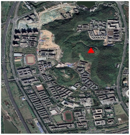
Figure 1.
Satellite cloud image of Nanjing University (The triangle in the figure is the weather tower).
2.2. Numerical Simulation Settings
Referring to the previous methods, the WRF–CFD coupling simulation method is used in this paper to provide boundary conditions for CFD simulation area through WRF simulation results.
WRF Mode Settings
In this study, the WRF–ARW model with multi-scale interaction capability was used to generate the meteorological background. As shown in Figure 2, the four-level nested one-way domain from East China to Nanjing University is considered with horizontal resolutions of 27 km, 9 km, 3 km, and 1 km, respectively. The center of the WRF simulation area is located at the Xianlin campus of Nanjing University (lat = 32.118, lon = 118.957). The grid points of the four nested domains Domain 1 (D1), Domain 2 (D2), Domain 3 (D3) and Domain 4 (D4) are 100 × 100, 112 × 112, 121 × 121 and 151 × 151, respectively. There are 40 terrain-based pressure layers from the ground to 50 hPa in the vertical direction and the lowest 21 layers used to provide CFD boundary conditions are all below 1 km. The WRF mode was initialized using National Centers for Environmental Prediction (NCEP) Final Analysis (FNL) data at 1 × 1 degree 6 h resolution. The simulation results of the WRF model are saved every 10 min during the period of interest (12:00 on 9 August 2020 to 24:00 on 10 August 2020). The physics schemes available in WRF–ARW were carefully chosen to better simulate surface winds, temperature and other meteorological parameters, and the effects of radiation and clouds were taken into account.
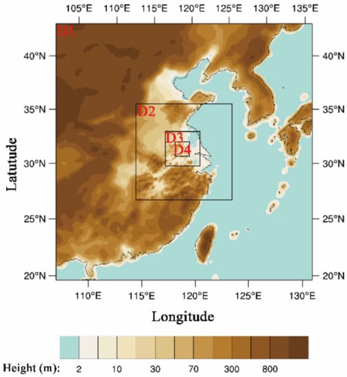
Figure 2.
Simulated domain of WRF model: scope of the four nested domains (D1–D4) used in the meteorological simulation.
Long-wave and short-wave radiation physics utilize the rapid radiative transfer model long-wave and Dudhia short-wave radiation schemes, respectively. The microphysical model adopts the WRF model’s single moment six-level scheme (WSM6), and the land surface flux adopts the unified Noah land surface model. The Mellor–Yamada–Janjic (MYJ) scheme and the corresponding MYJ Monin–Obukhov scheme are used for planetary boundary layer (PBL) turbulence and surface layer models. The cumulus parameterization models are not used in the two most refined domains: D3 and D4. The Kain–Fritsch scheme is used for the convective parameterization of the first and second domains.
2.3. CFD Simulation Settings
The computational domain uses the commercial CFD software Fluent 19.2 to solve the experimental case, which implements finite volume method (FVM) based on control volume. In order to more intuitively reflect the dispersion characteristics of heavy gases in complex environments, a simplified geoindicator simulation domain is established in this study. As shown in the Figure 3, the CFD domain is located in the middle part of the D4 area. The x axis represents the east–west direction, the y axis represents the north–south direction, and the z axis represents the vertical height. The length of the domain is 2404 m, the span of the domain is 1681 m, and the height is 1089 m.
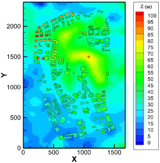
Figure 3.
CFD model diagram of computational domain.
The mesh with non-uniform structure is used to discretize the domain. Appropriate mesh refinement is performed in buildings, ground and SF6 release areas. Three kinds of meshing situations of mesh with non-uniform structure in the computational region are compared. When the number of meshes exceeds 1,691,426, the gas concentrations at the measurement points are practically consistent.
The CFD simulation was performed from 19:00 on 9 August 2020 to 21:00 on 9 August 2020, Beijing time. Buildings and ground are set as wall boundary conditions, establishing symmetry at the top of the domain. The setting of the inlet and outlet boundaries depends on the inlet wind direction. Gridded data from WRF, including wind direction (WD), wind speed (WS), and temperature (T), are stored at 10 min intervals during downscaling data transmission.
Wind speed and direction provide initial inlet conditions for the computational region through inverse interpolation as well as inlet boundary conditions for each time step. The temperature of computational domain was also offered by WRF simulation results.
Since the temperature changes little with time, the temperature at the inlet boundary during the simulation time is linearly fitted, and the fitting formula is: T = −0.00635Z + 303.1627. It is clear that the atmospheric stability was neutral during the experiment. In this study, simulations were first carried out based on real SF6 dispersion experiments. Next, in order to explore the influence of atmospheric stability on the flow field and pollutant distribution, the change in atmospheric stability was controlled by changing the vertical temperature gradient. The inlet wind speed is still simulated using the WRF results. The fitting formula for temperature under unstable conditions is changed to: T = −0.01935Z + 303.1627. The fitting formula for temperature under stable conditions is: T = 0.01635Z + 303.1627. Considering the balance between computational efficiency and accuracy, RANS (Reynolds-averaged Navier–Stokes) model was adopted for the simulation. The Navier–Stokes equations mainly consist of conservation equations for mass, momentum, energy and species concentration:
where is density and t is time.
where v is velocity, p is pressure, τ is shear stress and g is gravitational acceleration.
where and is the specific heat, T is the temperature and is the thermal conductivity.
where Y is the mass fraction and is the diffusion coefficient.
To solve the Navier–Stokes equations, several turbulence models are used in CFD. This study includes four main turbulence models, e.g., the renormalization group (RNG) k-ε model [23], realizable k-ε model [24], standard k-ε model [25] and shear stress transfer (SST) k-u model [26]. Detailed descriptions of the models can be found in the Fluent manual [27].
2.4. Description of Nanjing University Meteorological Tower Observation and SF6 Diffusion Experiment
There is a 75 m meteorological tower in the simulation area, which is used to collect meteorological data in the vertical direction of the study area, as shown in Figure 4.
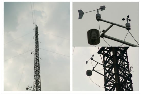
Figure 4.
Meteorological tower at Nanjing University.
The meteorological tower is located in the center of the WRF simulation area (lat = 32.118, lon = 118.957) and contains 4 floors (i.e., 9 m, 18 m, 36 m, 54 m). Each layer can continuously measure WS, WD and temperature (T). To validate the accuracy of the WRF simulation, the WS, WD and T data at 9 m, 18 m, 36 m and 54 m from the SF6 diffusion experiment were used in this study.
In order to study the diffusion behavior of gaseous substances on the real complex underlying surface, an SF6 tracer experiment was carried out. The density of SF6 (6.164 kg/m3) is about 5 times that of air. It is a highly inert and non-toxic gas. The concentration of SF6 is very low in the atmospheric environment and can be easily detected. Therefore, we used SF6 as a gas tracer in our experiments. The diffusion experiment of SF6 was conducted at Nanjing University from 19:16 on 9 August 2020 to 20:36 on 9 August 2020. as shown in Figure 5, SF6 was continuously emitted from the source at a constant source strength of 1.25 g/s. A total of 9 sampling points were set up in the experiment. These sampling points were determined according to the WS value and WD value at 1 h and were mainly distributed in the open space between school roads, public places and buildings. The wind direction during the test was mainly south–west, so the sampling points were selected at the downwind position. The release time of SF6 was 80 min in total. Twelve time points were sampled and a total of 108 samples were collected from nine sampling sites. In order to verify the accuracy of the WRF model coupled with the CFD model, the SF6 concentrations collected at nine sampling points were averaged (validation section in Section 3.1.2). After SF6 release, samples were taken using the CCZ10 sampler with a flow rate of 1 L/min per site. Each sample was collected using a 5 L Teflon gas sampling bag. All samples were analyzed by SP3420A gas chromatograph.
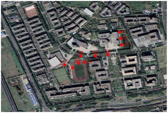
Figure 5.
Location of release and sampling points in the experiment (pentagram is the release point; dots are sampling points).
3. Results and Discussion
3.1. Validation of Simulation Results
3.1.1. Comparison of Simulations and Observations of the WRF Model
In order to quantitatively evaluate the error between the experimental and simulated data, a set of statistical performance methods proposed by Simon et al. [28] was adopted to evaluate the WRF numerical simulation results. Statistical performance indicators include fractional mean error (ME), root-mean-square error (RMSE), normalized mean error (NME), mean normalized error (MNE), and bias (FB). These measures have been widely used in atmospheric diffusion models. It can be seen from Table 1 that the WS observed in the meteorological tower of Nanjing University during the experiment is small, and the maximum value is 1.62 m/s. Obviously, the observed WS increases with increasing height. Combined with Figure 6, it can be seen that the WRF simulation results are slightly larger than the meteorological tower observation results. With the increase in height, various statistical parameters are significantly improved, which may be related to the complexity of the urban underlying surface. It can be seen from Table 1 that during the experiment, the WD observed in the meteorological tower at Nanjing University is generally in the southwest wind direction, and the wind direction fluctuates around 195°. The observed WD does not change much with the increase in height. Combined with Figure 7, it can be seen that the minimum error of MEAN is 1° and the maximum is 7°, and the maximum and minimum values of RMSE are 33.16 and 37.26. Comparative analysis shows that the overall trend of WRF’s simulation for wind direction is relatively close, but there is still a certain error.

Table 1.
Statistical evaluation of WRF simulation results.
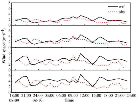
Figure 6.
WRF simulated wind speed and observed wind speed at different heights (9 m, 18 m, 36 m, 54 m from top to bottom).
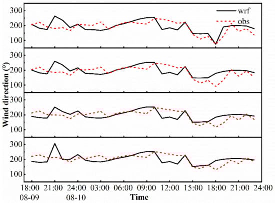
Figure 7.
WRF simulated wind direction and observed wind direction at different heights (9 m, 18 m, 36 m, 54 m from top to bottom).
3.1.2. Comparison of Simulations and Observations of the SF6 Concentrations near the Ground
In order to quantitatively evaluate the error between the experimental and simulated data, a set of statistical performance methods proposed by Chang and Hanna [29] was adopted to evaluate the numerical simulation results of different turbulence models. Statistical performance indicators included fractional bias (FB), normalized mean squared error (NMSE), correlation coefficient (R), simulated scores within two observed factors (FAC2), and simulated scores within five observed factors (FAC5). These measures have been widely used in atmospheric diffusion models.
In this study, SF6 was collected at a distance of 20 cm from the ground and its concentration was measured. A total of 12 sets of data were collected during the experiment and averaged to compare them with the simulated SF6 concentrations. The predicted concentrations of four RANS turbulence models were validated based on experimental data from nine sampling points. The agreement between the calculated results and the experimental data was quantified using model performance indicators, and the results are shown in Table 2. Chang and Hanna [29] suggested using the following measurement range to represent “acceptable model performance”: −0.3 < FB < 0.3, NMSE < 4, FAC2 > 0.5. Good statistical performance is shown for the renormalization group k-ε and SST models, while the standard k-ε and RNG k-ε models perform poorly. On the whole, the realizable k-ε model was used in this study, and its various indicators performed well, with a fractional deviation (FB) of 0.06, an NMSE of 0.35, a correlation coefficient (R) of 0.64 and FAC2 of 0.78.
Table 2.
Statistical evaluation of simulation results of different turbulence models.
3.2. Distribution Characteristics of Wind Field and Pollutant Concentration with Different Degrees of Stability and Different Heights
In this study, numerical experiments of CFD under different atmospheric stability (unstable, neutral and stable) were established. Figure 8 shows the simulated concentration (ppb) and wind vector fields at two altitudes at 19:24 LST on 9 August 2020. At this point, the environmental wind direction given by the WRF model is southwest. The study found that the wind vector inside the building is very different from the free wind vector in the boundary area. Comparing the wind fields at different heights, it is found that the overall wind speed at z = 21.5 m is higher than that at z = 1.5 m, and the influence of buildings on the wind direction is more significant at lower heights (z = 1.5 m).
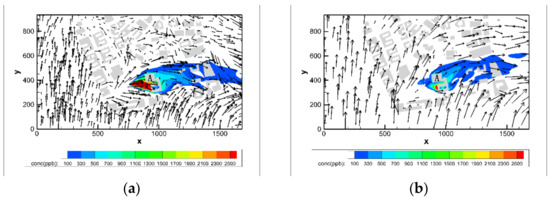
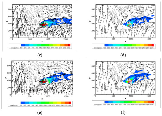
Figure 8.
Simulated concentrations (ppb) and wind vector fields of the LST at 20:08, 9 August LST. The arrow shows the wind: (a,c,e) at z = 1.5 m; (b,d,f) at z = 21.5 m; (a,b) unstable condition; (c,d) neutral condition; (e,f) stable condition.
The wind vector diagram shows that under unstable conditions, turbulence is generated by a combination of mechanical processes and thermal effects, and the incoming wind is deflected to a certain extent before encountering the building group. When the ambient wind enters the street between the buildings in the southwest at a certain angle, it can be seen from the upper-air chart that a spiral airflow is formed here, and the airflow is transported along the street valley and is reflected as a complex of crossed vortex and pipe flow in the street valley. The airflow eventually generates a flow around the building. As the stability increases, the turbulent effect is weakened, and the low wind speed area affected by the building is more significant. Under steady conditions, turbulent flow is mainly produced by mechanical processes. The magnitude of wind direction deflection decreases, and the change of the spiral airflow structure causes the wind direction near the pollution source to shift slightly to the north. Because the buildings are more sparsely distributed at the height of 21.5 m, the wind field there is stronger and simpler. With the increase of atmospheric stability, areas with high density of buildings are more likely to form low wind speed areas, such as the wind vector around buildings in the northwest and building A.
The SF6 concentration diagram shows that the high concentration area mainly appears in the upwind direction of building A, which indicates that pollutants are mainly accumulated here due to the hindrance of building A. The area at concentration (CONC) > 200 ppb under unstable conditions is smaller than that under neutral and stable conditions, and the pollutant plume is mainly diluted by strong turbulent mixing. When the atmosphere is in a steady state, the decrease in the deflection angle of the incoming wind leads to the northward development of the pollutant plume, and the weakening of the turbulent effect leads to the increase in the pollutant plume range near the ground and high in the air.
At 20:40 LST, the ambient wind speed increased and the wind direction changed to the southeast (Figure 9). When the incoming wind encountered the buildings in the southwest, it flowed around the building group, so that the westerly wind with different deflections was formed around the pollution source. Under unstable conditions, the strong thermal turbulence enhances the vortex intensity and plume dilution near the building. The pollutants are fully diluted, and the pollutants on the breathing surface mainly accumulate on the leeward side of building A. The pollutants in the high air with Z = 21.5 m mainly accumulated on the north side of building A. When the atmospheric conditions are neutral, the pollutant concentrations and the distribution characteristics of wind vectors are similar to those of unstable conditions. Due to the relatively weak turbulent motion, the area at concentration (CONC) > 50 ppb in the computational domain increases. When the atmospheric conditions are stable, the stable thermal stratification increases the horizontal conveying and suppresses the vertical movement of the airflow, so the scope of the pollutant plume at the breathing surface expands, and the maximum value of the pollutant concentration at the leeward side of building A increases. It is worth noting that, at the altitude of Z = 21.5 m, the peak of pollutant concentration increased but the range of pollutant plume decreased.
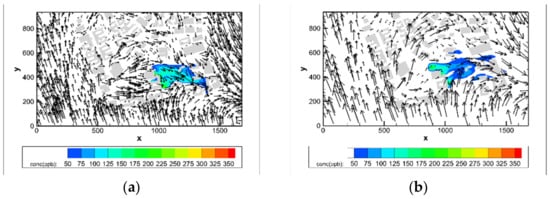
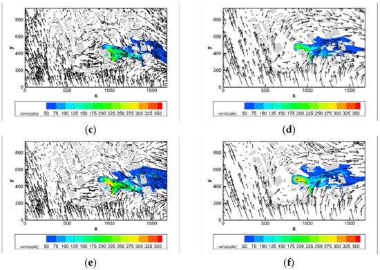
Figure 9.
Simulated concentrations (ppb) and wind vector fields of the LST at 20:40, 9 August LST: (a,c,e) at z = 1.5 m; (b,d,f) at z = 21.5 m; (a,b) unstable condition; (c,d) neutral condition; (e,f) stable condition.
3.3. Distribution Characteristics of Vertical Wind Field with Different Degrees of Stability
In order to study the influence mechanism of atmospheric stability on air circulation, the streamlines of the wind flow in the x-z section through the geometrical center released by SF6 are shown in Figure 10, and the vertical wind speed passing through is indicated in color in the figure. Under different conditions, the computational domain as a whole behaves as an upward wind. Stable stratification suppresses airflow movement in the vertical direction. Under unstable and neutral conditions, the airflow moves strongly in the vertical direction. For example, it is observed that there is an obvious positive upward flow zone on the windward side of building A, and it reaches its maximum value above the windward side of building A, which is related to the upward forcing effect on the windward side of building A, which is particularly significant under the conditions of unstable and neutral atmosphere. Under stable conditions, there is a strongly downward moving air zone on the leeward side of building A. The decrease in airflow on the leeward side of building A can explain the decrease in the air ventilation ability in the wake area of building A under unstable conditions because they lower the high-altitude hot air to a height close to the ground, which leads to a temperature gradient in the flow direction and weakens the dilution effect near the ground and makes it difficult for the pollutants to be sufficiently diluted. Therefore, it should be clear that thermal stratification of the atmosphere can have a significant impact on the flow field of the urban complex underlying surface. This presents significant challenges to the prediction of accidental release of hazardous substances and the timely implementation of remedial measures. Therefore, the CFD study of such structures cannot be limited to the neutral atmosphere because the leakage time of harmful gases is contingent, and it is particularly important to conduct a series of numerical simulation calculations for different degrees of stability.
Figure 10.
Streamline diagram and vertical wind speed at 19:24 LST on 9 August: (a) unstable condition; (b) neutral condition; (c) stable condition.
3.4. Concentration Characteristics of Different Stability and Different Heights
Figure 11 compares the area at CONC ∈ [150 ppb, 200 ppb] and the area at CONC ∈ [300 ppb, +∞) under different atmospheric conditions and different heights. In the high concentration area, when height = 0.2 m, the areas under unstable, neutral and stable conditions are 92, 5184 and 12,362, respectively. Under unstable and neutral conditions, with the increase in height, the area of the high-concentration region first decreases, then increases, and finally decreases. When the atmospheric conditions are stable, due to the weak dilution ability of the atmosphere, the area of each concentration interval of SF6 is the largest, and the maximum value of the high concentration area appears at height = 20 m. When height = 0.2 m, in the low concentration area, the areas under unstable, neutral and stable conditions are 21,703, 61,479 and 85,404, respectively. It is worth noting that under different conditions, the area of the low concentration area appears as an extreme value when height = 50 m, which is mainly related to the high-speed static pressure zone formed at the sharp corner of building A.
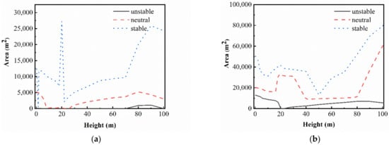
Figure 11.
Areas of each concentration interval of SF6 under different heights at 20:40 LST on August 9: (a) CONC ∈ [150 ppb, 200 ppb]; (b) CONC ∈ [300 ppb, +∞).
Figure 12 compares the highest concentrations of SF6 under different heights and different atmospheric conditions at 20:08 LST and 20:40 LST. At 20:08 LST, when the height is from 0.2 m to 90 m, the SF6 concentration is the largest under stable condition, and when the height is from 140 m to 200 m, the SF6 concentration under unstable condition is the largest, which is related to the stable temperature stratification that suppresses vertical turbulence, and a similar phenomenon also occurs at 20:40 LST. Therefore, stable atmospheric stratification is not conducive to the diffusion of harmful substances into the air. When the leakage of hazardous substances occurs on cloudless nights, relevant personnel should pay sufficient attention to it.
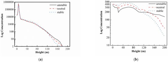
Figure 12.
The maximum concentration of SF6 at different altitudes:(a) 20:08 LST; (b) 20:40 LST.
4. Conclusions
In this paper, the WRF–CFD method was used to study the influence of atmospheric stability on the diffusion of hazardous substances on the urban complex underlying surface. Nanjing University was selected as the case study area, and the buoyancy caused by atmospheric temperature property was simulated by changing the vertical temperature gradient. The WRF simulation results were validated by the meteorological tower at Nanjing University and used the inverse distance interpolation method as the boundary condition of the CFD model. According to the field test results, the statistical parameters of different turbulence models were verified, and the realizable k-ε model was selected for simulation. By analyzing the wind field, tracer plume and tracer distribution characteristics at different heights, the influence of atmospheric stability on the leakage of hazardous substances was explored, and the following conclusions were drawn.
Changes in the environmental wind direction can significantly affect the diffusion model of pollutants, and changes in atmospheric stability can cause a certain degree of deflection of the environmental wind direction. Under unstable atmosphere, thermal turbulence deflects the ambient wind direction.
At the same time, atmospheric stability plays a crucial role in the pollution within the building group, which determines the potential turbulent diffusion capacity of the atmospheric surface. For example, under the stable atmospheric boundary condition, although the change of the environmental wind direction brings certain changes to the flow field structure in the building group, due to the weak turbulent diffusion, the SF6 plume under the stable condition has a higher area at 20:08 LST and 20:40 LST.
Stable atmospheric stratification suppresses vertical turbulence. The dilution ability under the unstable condition is the strongest. During the release of SF6, SF6 is diluted near the altitude of about 100 m due to the influence of vertical diffusion. SF6 concentration is lowest under the unstable condition 8 min after SF6 release is stopped.
In conclusion, the severity of the consequences of accidental release of hazardous substances is significantly affected by atmospheric stability, especially in complex urban buildings. Currently, the research in this field is still a blank, and more types of atmospheric stability deserve to be studied. In addition, the WRF-coupled CFD model is also capable of exploring the influence of other influencing factors on the diffusion of hazardous substances.
Author Contributions
Conceptualization, H.Z. and K.X.; methodology, H.Z. and K.X.; software, H.Z.; validation, H.Z., W.S. and K.X.; formal analysis, H.Z. and K.X.; investigation, H.Z., W.S. and K.X.; writing—review and editing, H.Z.; supervision, W.S. and K.X. All authors have read and agreed to the published version of the manuscript.
Funding
This research received no external funding.
Institutional Review Board Statement
Not applicable.
Informed Consent Statement
Not applicable.
Data Availability Statement
Not applicable.
Conflicts of Interest
The authors declare no conflict of interest.
References
- Gao, P.; Li, W.; Sun, Y.; Liu, S. Risk assessment for gas transmission station based on cloud model based multilevel Bayesian network from the perspective of multi-flow intersecting theory. Process Saf. Environ. Prot. 2022, 159, 887–898. [Google Scholar] [CrossRef]
- Li, Q.; Zhou, S.; Wang, Z. Quantitative risk assessment of explosion rescue by integrating CFD modeling with GRNN. Process Saf. Environ. Prot. 2021, 154, 291–305. [Google Scholar] [CrossRef]
- Sarvestani, K.; Ahmadi, O.; Mortazavi, S.B.; Mahabadi, H.A. Development of a predictive accident model for dynamic risk assessment of propane storage tanks. Process Saf. Environ. Prot. 2021, 148, 1217–1232. [Google Scholar] [CrossRef]
- Huimin, G.; Lianhua, C.; Shugang, L.; Haifei, L. Regional risk assessment methods in relation to urban public safety. Process Saf. Environ. Prot. 2020, 143, 361–366. [Google Scholar] [CrossRef]
- Allegrini, J.; Dorer, V.; Carmeliet, J. Wind tunnel measurements of buoyant flows in street canyons. Build. Environ. 2013, 59, 315–326. [Google Scholar] [CrossRef]
- Shen, Z.; Cui, G.; Zhang, Z. Turbulent dispersion of pollutants in urban-type canopies under stable stratification conditions. Atmos. Environ. 2017, 156, 1–14. [Google Scholar] [CrossRef]
- Yassin, M.F. Experimental study on contamination of building exhaust emissions in urban environment under changes of stack locations and atmospheric stability. Energy Build. 2013, 62, 68–77. [Google Scholar] [CrossRef]
- Guo, D.; Zhao, P.; Wang, R.; Yao, R.; Hu, J. Numerical simulations of the flow field and pollutant dispersion in an idealized urban area under different atmospheric stability conditions. Process Saf. Environ. Prot. 2020, 136, 310–323. [Google Scholar] [CrossRef]
- Zhou, X.; Ying, A.; Cong, B.; Kikumoto, H.; Ooka, R.; Kang, L.; Hu, H. Large eddy simulation of the effect of unstable thermal stratification on airflow and pollutant dispersion around a rectangular building. J. Wind Eng. Ind. Aerodyn. 2021, 211, 104526. [Google Scholar] [CrossRef]
- Duan, G.; Ngan, K. Influence of thermal stability on the ventilation of a 3-D building array. Build. Environ. 2020, 183, 106969. [Google Scholar] [CrossRef]
- Dai, T.; Liu, S.; Liu, J.; Jiang, N.; Liu, W.; Chen, Q. Evaluation of fast fluid dynamics with different turbulence models for predicting outdoor airflow and pollutant dispersion. Sustain. Cities Soc. 2022, 77, 103583. [Google Scholar] [CrossRef]
- Cui, P.-Y.; Zhang, Y.; Chen, W.-Q.; Zhang, J.-H.; Luo, Y.; Huang, Y.-D. Wind-tunnel studies on the characteristics of indoor/outdoor airflow and pollutant exchange in a building cluster. J. Wind Eng. Ind. Aerodyn. 2021, 214, 104645. [Google Scholar] [CrossRef]
- Zheng, X.; Yang, J. CFD simulations of wind flow and pollutant dispersion in a street canyon with traffic flow: Comparison between RANS and LES. Sustain. Cities Soc. 2021, 75, 103307. [Google Scholar] [CrossRef]
- Du, Y.; Blocken, B.; Pirker, S. A novel approach to simulate pollutant dispersion in the built environment: Transport-based recurrence CFD. Build. Environ. 2020, 170, 106604. [Google Scholar] [CrossRef]
- Hu, Y.; Wu, Y.; Wang, Q.; Hang, J.; Li, Q.; Liang, J.; Ling, H.; Zhang, X. Impact of Indoor-Outdoor Temperature Difference on Building Ventilation and Pollutant Dispersion within Urban Communities. Atmosphere 2022, 13, 28. [Google Scholar] [CrossRef]
- Miao, Y.; Liu, S.; Chen, B.; Zhang, B.; Wang, S.; Li, S. Simulating urban flow and dispersion in Beijing by coupling a CFD model with the WRF model. Adv. Atmos. Sci. 2013, 30, 1663–1678. [Google Scholar] [CrossRef]
- Kadaverugu, R.; Purohit, V.; Matli, C.; Biniwale, R. Improving accuracy in simulation of urban wind flows by dynamic downscaling WRF with OpenFOAM. Urban Clim. 2021, 38, 100912. [Google Scholar] [CrossRef]
- Temel, O.; Bricteux, L.; van Beeck, J. Coupled WRF-OpenFOAM study of wind flow over complex terrain. J. Wind Eng. Ind. Aerodyn. 2018, 174, 152–169. [Google Scholar] [CrossRef]
- San José, R.; Pérez, J.L.; Gonzalez-Barras, R.M. Assessment of mesoscale and microscale simulations of a NO2 episode supported by traffic modelling at microscopic level. Sci. Total Environ. 2021, 752, 141992. [Google Scholar] [CrossRef]
- Wong, N.H.; He, Y.; Nguyen, N.S.; Raghavan, S.V.; Martin, M.; Hii, D.J.C.; Yu, Z.; Deng, J. An integrated multiscale urban microclimate model for the urban thermal environment. Urban Clim. 2021, 35, 100730. [Google Scholar] [CrossRef]
- Temel, O.; Porchetta, S.; Bricteux, L.; van Beeck, J. RANS closures for non-neutral microscale CFD simulations sustained with inflow conditions acquired from mesoscale simulations. Appl. Math. Model. 2018, 53, 635–652. [Google Scholar] [CrossRef] [Green Version]
- Li, S.; Sun, X.; Zhang, S.; Zhao, S.; Zhang, R. A Study on Microscale Wind Simulations with a Coupled WRF–CFD Model in the Chongli Mountain Region of Hebei Province, China. Atmosphere 2019, 10, 731. [Google Scholar] [CrossRef] [Green Version]
- Yakhot, V.; Orszag, S.A.; Thangam, S.; Gatski, T.B.; Speziale, C.G. Development of turbulence models for shear flows by a double expansion technique. Phys. Fluids A 1992, 4, 1510–1520. [Google Scholar] [CrossRef] [Green Version]
- Shih, T.-H.; Liou, W.W.; Shabbir, A.; Yang, Z.; Zhu, J. A new k-ϵ eddy viscosity model for high reynolds number turbulent flows. Comput. Fluids 1995, 24, 227–238. [Google Scholar] [CrossRef]
- Brauer, H. Mathematical Models of Turbulence. Von B. E. Launder u. D. B. Spalding. Academic Press, London–New York 1972. 1. Aufl., V, 169 S., zahlr. Abb., geb., £ 2.50. Chem. Ing. Tech. 1973, 45, 143-143. [Google Scholar] [CrossRef]
- Menter, F.R. Two-equation eddy-viscosity turbulence models for engineering applications. AIAA J. 1994, 32, 1598–1605. [Google Scholar] [CrossRef] [Green Version]
- Ansys Inc. ANSYS FLUENT 14 User’s Guide; Ansys Inc.: Canonsburg, PA, USA, 2011. [Google Scholar]
- Simon, H.; Baker, K.R.; Phillips, S. Compilation and interpretation of photochemical model performance statistics published between 2006 and 2012. Atmos. Environ. 2012, 61, 124–139. [Google Scholar] [CrossRef]
- Chang, J.C.; Hanna, S.R. Air quality model performance evaluation. Meteorol. Atmos. Phys. 2004, 87, 167–196. [Google Scholar] [CrossRef]
Publisher’s Note: MDPI stays neutral with regard to jurisdictional claims in published maps and institutional affiliations. |
© 2022 by the authors. Licensee MDPI, Basel, Switzerland. This article is an open access article distributed under the terms and conditions of the Creative Commons Attribution (CC BY) license (https://creativecommons.org/licenses/by/4.0/).