A Novel Missing Data Imputation Approach for Time Series Air Quality Data Based on Logistic Regression

Abstract

Missing values in air quality datasets bring trouble to exploration and decision making about the environment. Few imputation methods aim at time series air quality data so that they fail to handle the timeliness of the data. Moreover, most imputation methods prefer low-missing-rate datasets to relatively high-missing-rate datasets. This paper proposes a novel missing data imputation method, called FTLRI, for time series air quality data based on the traditional logistic regression and a presented “first Five & last Three” model, which can explain relationships between disparate attributes and extract data that are extremely relevant, both in terms of time and attributes, to the missing data, respectively. To investigate the performance of FTLRI, it is benchmarked with five classical baselines and a new dynamic imputation method using a neural network with average hourly concentration data of pollutants from three disparate stations in Lanzhou in 2019 under different missing rates. The results show that FTLRI has a significant advantage over the compared imputation approaches, both in the particular short-term and long-term time series air quality data. Furthermore, FTLRI has good performance on datasets with a relatively high missing rate, since it only selects the data extremely related to the missing values instead of relying on all the other data like other methods.

1. Introduction

Air pollutants pose significant threats to public health, especially the toxicity and diseases caused by atmospheric fine particulate matter [1]. According to a survey, air pollution kills approximately 4.2 million people every year [2]. Therefore, air quality is still an issue of concern in recent years. Environmental researchers mine air quality data to uncover potential value and information, which captures user behavior [3], estimates influenza diseases [4], explores greenhouse gas emissions [5], investigates personal actions to reduce greenhouse gas emissions [6], and so on, to advise the related policy makers. However, due to problems of instrument malfunction, communication noise, and/or other unknown reasons [7], data are frequently missing. Moreover, although most air quality monitoring data are time series data, processing extensive time series environmental data with missing values is usually laborious and difficult, and sometimes unexpected failures are not detected until data are processed. Consequently, environmental databases frequently have some gaps caused by missing data [8]. It is the gap that not only seriously affects the accuracy and availability of data, but also affects the subsequent work of in-depth analysis and data mining [9]. Therefore, it is worthwhile to understand the types of data with missing values and propose an effective and robust strategy to fill time series air quality data with missing values.

In terms of the research of Rubin et al. [10], there are three types of data with missing values: Missing Completely at Random (MCAR), Missing at Random (MAR), and Not Missing at Random (NMAR). When data are MCAR, the fact that the data are missing is independent of the observed and unobserved data [10,11]. When data are MAR, the fact that the data are missing is systematically related to the observed but not the unobserved data [10,12]. When data are NMAR, the fact that the data are missing is systematically related to the unobserved data, that is, the missingness is related to events or factors that are not measured by the researcher [10,13]. Following these three categories, there are some efficient strategies to coordinate data with missing values, appropriately known as “imputation methods” [14]. Mean imputation and Median imputation are two common missing value imputation methods when data are MCAR. They are used as benchmark methods for imputing missing values in air quality datasets in many studies, such as [15,16,17,18,19]. They substitute the mean or median of the corresponding observed attribute’s values for the missing values of that attribute in a dataset, respectively [20]. However, these two simple imputation strategies lose sight of the correlation between the missing value’s own attribute and other attributes in the data points. k-nearest neighbor imputation [21] and random forest imputation [22] are two typical missing value imputation methods when data are MAR. They take into account the dependencies among different attributes of data points, and the missing value of a data point can be obtained according to other data points with complete values. In the k-nearest neighbor imputation method, the missing attribute values in a data point are replaced by the average of the corresponding attribute values of k nearest neighbors of the data point [21,23]. It has been proven that k-nearest neighbor has good imputation performance for air quality data in the literature [15,16]. Researchers [24] have proven that the imputation performance of random forest outperforms k-nearest neighbor due to its being a combination of tree predictors, where each tree depends on a random data point sampled independently [22,25]. However, an air quality monitor runs as a time series and can generate large amounts of missing data sometimes. The missing data mechanism of air quality data is generally random (MAR—missing at random) [19]. The above methods are most capable in datasets with a low missing rate, but they may provide a poor performance on a large number of discrete datasets with a relatively high missing rate [26]. Moreover, without considering that the timeliness among data points also affects data quality in a dataset, these methods may be not suitable for time series data. When processing time series datasets, these methods usually require a large number of training data points to establish a low imputation error model, because they ignore the fact that time series data points are correlated with each other over continuous time intervals, namely, the data differ less in value in short time intervals since the time corresponding to the data point is continuous. Therefore, to solve the issues of missing values in time series air quality data, it is necessary to further explore a more suitable imputation method for time series air quality data with missing values, which not only can train a higher imputation performance model with fewer air quality data, but also can achieve more efficient imputation for relatively high-missing-rate time series air quality datasets with discrete missing values.

In this paper, to achieve more efficient imputation of discrete missing values in time series air quality data, we raise a new single imputation method [18,27] called “First five last three logistic regression imputation (FTLRI)”. This method combines the traditional logistic regression with a presented “first Five & last Three” model, which can explain relationships between/among disparate attributes and extract the data points that are extremely relevant, both in terms of time and attributes, to the data point with missing values, respectively.

Since timeliness of data points in a dataset in an important factor affecting data quality [28], FTLRI uses a model of “first Five & last Three (FT)” to address that issue based on the sliding window, where “F” refers to the five data points with complete values immediately before the data point with missing values, and “T” refers to the three data points with complete values immediately after the data point with missing values in a time series dataset. Selecting the first five and the last three data points next to the data point with missing values ensures commonality of experience between data points, and the eight data points are most closely related in time to the missing value. In addition, to fully consider the correlation between different attributes in the data points, FT selects the attributes extremely related to the attribute with missing values based on the Pearson correlation. Therefore, FT emerges as a time-dependent and attribute-related model, which chooses the most appropriate, minimal amount of data to set the basis for the subsequent, most efficient missing data imputation.

To further fully use correlation between continuous time and the different attributes of data points in air quality data, these eight data points with complete values selected by FT are employed in logistic regression to train a model to fill missing values effectively. Logistic regression has been widely studied recently, such as parameter estimation [29], credit scoring [30], visual detectability prediction [31], and so on, but few studies have examined the application of logistic regression to missing data, let alone its application to fill time series air quality data. Although Akbar et al. [32] indicated that random forest is more accurate than traditional logistic regression imputation for data with missing values, they did not make a detailed analysis of the two approaches. As an imputation method under the category MAR, logistic regression imputation warrants further investigation in time series air quality data with missing values for the declarative reasons. One is that logistic regression is used to explain the relationship between one dependent attribute and one or more independent attributes by estimating probabilities using a logistic regression equation in the description and analysis of data [33]. There is an interaction among the six main pollutants in the air quality data points. For example, the concentration of PM_2.5 may be affected by the concentration of the other pollutants, such as SO₂, CO, and NO₂ [34]. The second is that logistic regression does not require high computing power, and low-performance equipment can complete the calculation [35].

To investigate the performance of FTLRI, this paper compares the three assessment indexes of FTLRI with five other classical imputation methods and a new dynamic imputation method [36] using a neural network with missing rates of 5%, 10%, 20%, and 40%, respectively, and demonstrates that the performance of FTLRI is superior to the others. Overall, the main advantages of FTLRI are as follows.

(1)

FTLRI is an effective time series air quality data imputation model that not only considers correlation, both in terms of time and attributes of the data points, but also legitimately utilizes logistic regression to deal with such correlation.

(2)

FTLRI relies on fewer training data points for each data point with missing values, including eight data points extremely relevant to the data point with missing values, to achieve a lower imputation error model compared with the other classical imputation methods.

(3)

FTLRI realizes accurate imputation of short-term/long-term time series air quality datasets with different missing rates by extracting the data points that are extremely relevant, both in terms of time and attributes, to the data point with missing values.

2. Materials and Methods

This section will illustrate the imputation method FTLRI proposed in this paper and the indicators to evaluate the performance of FTLRI.

2.1. A Developed FT Based on Pearson Correlation and Sliding Window

Time series air quality data are time-dependent and attribute-related. To better understand how to extract the data that are highly relevant to missing data through “first Five & last Three (FT)” in time series datasets, this subsection elaborates the developed model FT covering the Pearson correlation and a sliding window.

The Pearson correlation is employed to reveal the attributes that are highly relevant to the attribute with missing values in a time series dataset in this paper. The Pearson correlation coefficient indicates a linear relation between two attributes in a dataset, and it ranges from −1 to +1. The greater the absolute value of the correlation coefficient is, the higher the correlation degree of the two attributes in a dataset will be [37]. In this study, if the Pearson correlation coefficient between an attribute and the attribute with missing values is greater than or equal to 0.6, then the attribute is regarded as a target attribute of the attribute with missing values. It is assumed that the concentration of one pollutant at a certain time is p and the concentration of another pollutant at the same time is q in a time series air quality dataset containing n data points; then, the Pearson correlation coefficient r of the two pollutants can be expressed as Equation (1). The process of filtering the target attributes of the attribute with missing values through the Pearson correlation coefficients is first done through FT, that is, the selected target attributes through FT first are the attributes that are extremely related to the attribute with missing values.

$$r_{pq}=\frac{n{{\displaystyle \sum }}_{t=1}^n{p}_t{q}_t-{{\displaystyle \sum }}_{t=1}^n{p}_t{{\displaystyle \sum }}_{t=1}^n{q}_t}{\sqrt{n{{\displaystyle \sum }}_{t=1}^n{p}_t^2-{\left({{\displaystyle \sum }}_{t=1}^n{p}_t\right)}^2}\sqrt{n{{\displaystyle \sum }}_{t=1}^n{q}_t^2-{\left({{\displaystyle \sum }}_{t=1}^n{q}_t\right)}^2}}$$

(1)

A sliding window is employed to seek out the data points that are highly relevant in time to the data point with missing values in a time series dataset in this paper. As shown in Figure 1, assuming that the concentration of one pollutant measured at time t is X(t), a sliding window refers to a window with size w that is used to slide from the starting point of a time series air quality dataset to the end with a step length of l, and the values in the window are recorded for subsequent research when the window moves forward. The missing data in a time series dataset may lead to incomplete data in the sliding window. The proposed model FT focuses on the imputation of the missing data through the complete data in the sliding window, which are closest in time. Through the sliding window, the “first Five” data points and the “last Three” data points with complete values closest in time to the data point with missing values are found, which is required for the second step of the model FT.

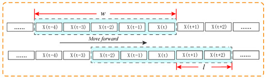
Figure 1. The schematic of a sliding window.

Instead of depending on all the other complete data like other methods to fill missing values, FT screens out the data that are highly correlated with the missing data, both in terms of attributes and time, in a time series air quality dataset to ensure a more effective imputation later. The basic steps of FT are as follows.

Step 1. 

If the Pearson correlation coefficient between an attribute and the attribute with a missing value is greater than or equal to 0.6, then this attribute is a target attribute.

Step 2. 

Find the “first Five (F)” data points and the “last Three (T)” data points close in time to the data point with missing values by a sliding window based on the first step, if and only if F and T are the data points with complete values composed of target attributes and attributes with missing values in a time series air quality dataset.

In Step 2, if a data point with missing values is followed by another data point with missing values for the corresponding attribute, then the search continues until the eight data points with complete values are discovered. Thus, there are two cases for the step length l and size w of the sliding window. The first one is that the step length l and size w of the sliding window are fixed, in which the sliding window size is 9. To test the performance of the imputation method proposed in this paper under different missing rates, the step length l of the sliding window is calculated according to the number of the data points and self-defined missing rate in a time series dataset. Assuming that there are n data points in a time series air quality dataset, and the self-defined missing rate is R, the step length can be expressed as Equation (2). The second case is that the step length l and size w of the sliding window are unfixed. When one of the three data points immediately behind the data point with missing values in time has a missing value for the corresponding attribute, it will continue to look for a data point with complete values. This is the reason the size w and the step length l of the window will increase by one. Therefore, we can obtain eight data points with complete values highly relevant to the data point with missing values in time through FT, which will alter as the data point with missing values alters in a time series air quality dataset.

$$l=\left[\frac{1}{R}\right]$$

(2)

The data selected through FT are extremely attributively and temporally related to each missing data point. In other words, for each data point with missing values, we search for the eight highly correlated data points through FT, which is more targeted and offers the possibility for more effective imputation in the follow-up.

By training an imputation model with the eight data points from FT for each data point with missing values, we not only can overcome the obstacle of other methods that demand large volumes of training data points to build a highly effective model, but also can save the time of training, especially for low-missing-rate datasets with discrete missing values. Thus, it is worth adopting FT into the imputation of time series air quality data with discrete missing values.

2.2. Logistic Regression Imputation

Since there exists a certain relationship between missing values and complete values in data points, this section will first introduce the idea of logistic regression and then describe how logistic regression is used to fill the missing values by employing this relationship.

Logistic regression includes three steps: finding a prediction function, constructing a loss function, and finding regression parameters that minimize a loss function [38,39]. The objective function of logistic regression is expressed as Equation (3).

$$h_{\theta }\left(x\right)=\frac{1}{1+e^{-{\theta }^{T}x}}$$

(3)

where θ is an unknown vector of parameters to be determined, x = (x₁, x₂, … x_d), and d denotes data point x has d attributes. The loss function reflects the degree of model prediction error. Suppose there are n data points, then the average log-likelihood loss will be Equation (4).

$$J\left(\theta \right)=-\frac{1}{n}\left[{\displaystyle \sum }_{i=1}^n{y}^{\left(i\right)}log{h}_{\theta }\left(x^{\left(i\right)}\right)+\left(1-y^{\left(i\right)}\right)\log \left(1-h_{\theta }\left(x^{\left(i\right)}\right)\right)\right]$$

(4)

where y is a return variable with a value of 0 or 1. The regression parameter θ minimizes the loss function, which can be obtained by Gradient Descent [40] and Newton’s method [41] and so on. Newton’s method is adopted in this study. Newton’s method takes the second-order Taylor Formula of the function near the existing estimate of the minimum point and then finds the next estimate of the minimum point. Assuming θ_k is an estimate of the current minimum, then there will be Equation (5).

$$\phi \left(\theta \right)=J\left({\theta }^k\right)+J^{\prime }\left({\theta }^k\right)\left(\theta -{\theta }^k\right)+\frac{1}{2}{J}^{″}\left({\theta }^k\right){\left(\theta -{\theta }^k\right)}^2$$

(5)

Supposing φ′ (θ) = 0, there will be Equation (6).

$${\theta }^{k+}={\theta }^k-\frac{J^{\prime }\left({\theta }^k\right)}{J^{″}\left({\theta }^k\right)}$$

(6)

where k is the number of iterations. Equation (6) is the iterative updated equation. From Equations (5) and (6), we can see this study requires the objective function J(θ) to be second-order continuously differentiable.

This paper applies logistic regression to the imputation domain of missing values. For each data point with missing values in a time series air quality dataset, we rely on an objective regression equation to build a specific imputation model using eight corresponding highly relevant data points from FT. However, it is worth noticing that this study needs to convert the complete data of a missing attribute from continuous type into integer type since logistic regression is frequently employed to cope with classification. For example, when there are missing values in the concentration of PM_2.5, we need to convert the complete values in PM_2.5 into integer data before we use logistic regression to train an imputation model. That is, when using logistic regression to train an imputation model to impute continuous data, we need to preprocess the complete data of the missing attribute by scaling the complete continuous data up to a multiple of 10 to the nth power, or by other methods, to obtain integer data. Further, the integer data processed can be inputted into logistic regression to train an imputation model. Accordingly, for the missing values of the continuous attribute converted into integer type, after the imputed values are obtained through logistic regression, it is necessary to be restored to continuous type. It is the restored data that constitute the final imputation concentration values of this study.

2.3. FTLRI Based on FT and Logistic Regression

“First five last three logistic regression imputation (FTLRI)” integrates the FT proposed in Section 2.1 and the logistic regression introduced in Section 2.2 to fill the discrete missing values in a time series air quality dataset. FTLRI is inspired by the following two considerations, which are clearly shown in Figure 2. The first point is that time series data have the characteristic of autocorrelation; in other words, the attribute values of a data point are closely related to the corresponding attribute values of the other data points in a time interval. For example, the concentration value of PM_2.5 is closely related to the concentration values before and after it, namely, it is not independent. The second point is that there exists a kind of cross-influence relationship among air pollutants. For example, the concentration of PM_2.5 can be extremely correlated with the concentration of the other pollutants at the same time, such as CO and PM₁₀. Exploiting highly correlated relationships to fill discrete missing values in time series air quality datasets offers higher accuracy. Instead of depending on all the other complete data like other methods to fill missing values, FTLRI depends on these two correlations to utilize FT to extract the data points that are highly relevant to each data point with missing values. FTLRI also makes full use of logistic regression to train a suitable imputation model for each data point with missing values.

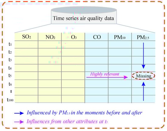
Figure 2. The illustration of FTLRI’s ideas.

The detailed procedure of FTLRI to impute data points with missing values is outlined in Algorithm 1. The process of FTLRI starts with an incomplete time series air quality dataset, and it takes no input parameters. By calculating the Pearson correlation coefficient, Step 1 can easily access the attributes highly relevant to the missing value attributes. Step 2 is based on Step 1 to search for the first five data points and the last three data points that are strongly related to the missing value in time by FT firstly. By finding the first five data points and the last three data points, then, we rely on logistic regression to train an imputer fitted to them. Finally, the missing values can be obtained by this imputer.

Algorithm 1 First five last three logistic regression imputation (FTLRI)

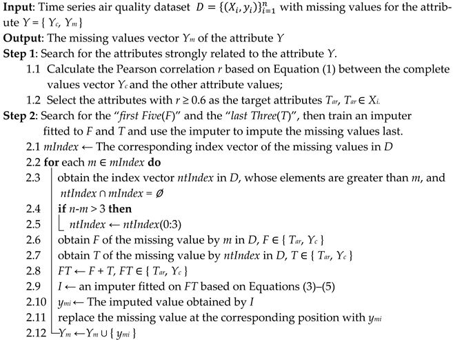Output Ym

Figure 3 illustrates the process of the imputation approach for a data point with missing values in more detail. We present only the attributes that are highly correlated with PM_2.5 in this figure, including CO and PM₁₀. In Figure 3, the missing value for the concentration of PM_2.5 is finally filled with “24”. First of all, by detecting the data point with a missing value and accessing its Pearson correlation coefficient, we can discovery the corresponding “first Five” and “last Three” of the data point, which are represented on the brownish-yellow background and blue-green background colors in the figure, respectively. Next, the “first Five” and the “last Three” are employed to train a model by logistic regression, and this model is applied to obtain the missing concentration values of PM_2.5 last; then, “24” is obtained.

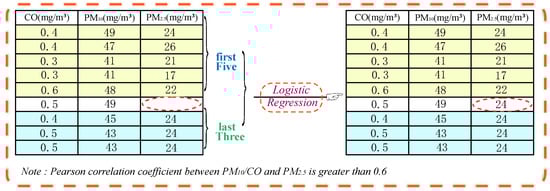
Figure 3. An example of FTLRI.

From the detailed explanation of the process in Figure 3, we can see that, in the process of training and filling through the model, it is the corresponding “first Five” and the “last Three” adjacent to each data point with missing values that simplify the training process of the imputation model and save training time.

Instead of depending on all the other complete data points like other methods, we select these eight data points highly relevant, both in terms of time and attributes, to each data point with missing values to fill missing values, which is the key of FTLRI to train a model with lower imputation errors through logistic regression under different missing rates.

2.4. Assessment Indexes

To evaluate the performance of FTLRI, three assessment indexes are used: Mean absolute error (MAE), Root-mean-square of error (RMSE) and Mean absolute percentage error (MAPE) [42,43,44], which are shown in the following Equations (7)–(9), respectively:

$$MAE=\frac{1}{n}{\displaystyle \sum }_{i=1}^n\left|r_i-f_i\right|$$

(7)

$$RMSE=\sqrt{\frac{1}{n}{\displaystyle \sum }_{i=1}^n{\left(r_i-f_i\right)}^2}$$

(8)

$$MAPE=\frac{100}{n}{\displaystyle \sum }_{i=1}^n\frac{\left|r_i-f_i\right|}{r_i}$$

(9)

where r and f are real and imputation values, respectively, and n denotes the number of a dataset with missing values.

3. Results and Discussion

In this section, to evaluate the effectiveness of FTLRI, we ran it on time series air quality datasets collected from Lanyuan Hotel (LH), Yuzhonglanda Campus (YZ), and Biological Products Institute (BPI) in Lanzhou in 2019. For data from each different station, we selected short-term and long-term time series air quality data with different missing rates, varying between 5%, 10%, 20% and 40%, to demonstrate the feasibility of FTLRI.

3.1. Data Preparation

To verify the performance of the proposed FTLRI approach, this study took hourly concentration (mg/m³) data from Lanzhou, an old industrial city in northwest China, as benchmarks, which contained SO₂, NO₂, O₃, CO, PM₁₀, and PM_2.5 at three stations, including LH, YZ, and BPI. Among the three stations, LH is located in Anning District, which integrates many colleges and universities, new technology, and culture, representing the main source of industrial pollution; YZ is located in the remote Yuzhong County, which expresses the background value of air quality; BPI is located in the urban area integrating commodities and housing, which reflects a high density of population and traffic pollution sources. The data came from “China Environmental Monitoring Station”, a website (http://www.cnemc.cn/ (accessed on 18 November 2020)) containing real-time measurements of concentrations of air pollutants for approximately 120 cities, embracing 600 monitoring stations. To make the study more persuasive, the study adopted the data from four different time series from March 2019, April to June 2019, July to December 2019, and the whole year of 2019 from the three above-mentioned stations and denoted them as T1, T2, T3, and T4, respectively, which is clearly shown in Table 1. Among them, time series T1 and T2 were employed to verify the performance of the imputation methods over a short term, while time series T3 and T4 were utilized to verify the performance of the imputation methods over a long term. The performance test of different imputation methods was carried out with PM_2.5 as an example.

Table 1. Notations and their explanations about data.

Notation	T1	T2	T3	T4
Meaning	March 2019	April to June 2019	July to December 2019	The whole year of 2019
	Short term	Short term	Long term	Long term

Prior to the experiment, all the data with missing values needed to be removed to avoid their influence on the accuracy of imputation results. In other words, the used data in this experiment were processed data with complete values [17,19]. Data information with complete values at the three different stations in the four disparate periods is shown in Table 2.

Table 2. Data information with complete values at different stations in different time series.

Stations	Time Series	Number of Datasets
LH	T1	722
	T2	2137
	T3	4185
	T4	8489
YZ	T1	699
	T2	1985
	T3	4161
	T4	8210
BPI	T1	680
	T2	1957
	T3	4076
	T4	8080

3.2. Pearson Correlation Coefficient between PM_2.5 and the Other Five Pollutants

Table 3 lists the Pearson correlation coefficient r between PM_2.5 and SO₂, NO₂, O₃, CO, and PM₁₀, respectively. In Table 3, the concentrations of PM_2.5 and PM₁₀ showed a strong correlation in four different time series at the three different stations in Lanzhou in 2019, and the correlation coefficient was positive, that is, r was greater than or equal to 0.6. This may be related to their relationship, namely, PM_2.5 is a kind of PM₁₀, and they have an inclusive relationship. PM_2.5 generally accounts for about 70% of PM₁₀ [45]. In addition, the concentrations of PM_2.5 also showed a strong correlation with CO in time series T3 and T4 at LH. There existed a strong correlation between PM_2.5 and SO₂, NO₂, and CO in time series T3 at YZ and BPI, respectively. To explain this correlation, we analyzed it in terms of time of year. T3, from July to December 2019, represents the last two quarters of the four seasons in a year. At this time, the overall temperature in Lanzhou gradually decreases so that people are more likely to choose motor vehicles as transportation tools. The main pollutants emitted by motor vehicles are CO, SO₂, and NO₂.

Table 3. Pearson correlation coefficient r between PM_2.5 and the other five pollutants in the short-/long-term time series.

Stations	Time Series	SO2	NO2	O3	CO	PM10
LH	T1	0.1603	0.5377	−0.2620	0.4664	0.6476
	T2	0.0455	0.1075	−0.0680	0.0971	0.9781
	T3	0.5753	0.5835	−0.3773	0.8444	0.8861
	T4	0.3693	0.4377	−0.2642	0.6263	0.8526
YZ	T1	0.1612	0.1517	−0.1014	0.0902	0.6475
	T2	−0.0134	−0.0168	−0.0650	−0.1014	0.9832
	T3	0.6115	0.6455	−0.4958	0.6018	0.7722
	T4	0.2924	0.2146	−0.2556	0.2872	0.8689
BPI	T1	0.1314	0.4347	−0.2114	0.3347	0.6035
	T2	−0.0353	0.1545	−0.1354	0.0922	0.9591
	T3	0.6666	0.7549	−0.4165	0.6979	0.8344
	T4	0.4416	0.5628	−0.3349	0.5555	0.7989

The implementation of the imputation experiment was carried out according to the Pearson correlation coefficients obtained in Table 3. We selected pollutants whose Pearson correlation coefficient with PM_2.5 was greater than or equal to 0.6 to fill the missing concentration values of PM_2.5 in Table 3. Specifically, at LH, the concentration values of PM₁₀ were employed to fill the missing concentration values of PM_2.5 through different imputation methods in time series T1 and T2, and the concentration values of CO and PM₁₀ were employed to fill the missing concentration values of PM_2.5 through different imputation methods in time series T3 and T4. At YZ, the concentration values of PM₁₀ were employed to fill the missing concentration values of PM_2.5 through different imputation methods in time series T1, T2, and T4, and the concentration values of SO₂, NO₂, CO, and PM₁₀ were employed to fill the missing concentration values of PM_2.5 through different imputation methods in time series T3. At BPI, the concentration values of PM₁₀ were employed to fill the missing concentration values of PM_2.5 through different imputation methods in time series T1, T2, and T4, and the concentration values of SO₂, NO₂, CO, and PM₁₀ were employed to fill the missing concentration values of PM_2.5 through different imputation methods in time series T3.

3.3. Imputation Results of Missing Concentration Values of PM_2.5

In this subsection, we will fully exhibit the imputation results for the time series air quality datasets with different missing rates at the three different stations.

To make the datasets containing n data points generate different missing rates, we removed the i × l (1 ≤ i < n × R + 1) data point in the corresponding dataset according to the step length l and missing rate R in Equation (2). For simplicity in graphs and tables, Table 4 shows the different imputation methods and their corresponding abbreviations used in this experiment. The number of neighbors for k-nearest neighbor was set to eight. The parameters of the random forest and logistic regression were almost set to default in the sklearn package in Python, except for solver = “newton-cg” in the logistic regression. For dynamic imputation, we used the Adam optimizer with a learning rate of 10⁻³ and a mini-batch size of 32, and we terminated the training when the number of epochs reached 500 [36].

Table 4. Abbreviations and their explanations about imputation methods.

Abbreviation	Explanation
MEAI	Mean Imputation
MEDI	Median Imputation
kNNI	k-Nearest Neighbor Imputation
LRI	Logistic Regression Imputation
RFI	Random Forest Imputation
DI	Dynamic imputation
FTLRI	First Five Last Three Logistic Regression Imputation

For the missing values of PM_2.5 concentration in the time series air quality dataset, we show the imputation results of the proposed method from three different perspectives. Table 5, Table 6 and Table 7 list the quantitative evaluations of the imputation results of different methods under different missing rates. Moreover, to see the imputation results of different methods more clearly, taking the missing rate of 5% as an example, Figure 4, Figure 5 and Figure 6 illustrate different methods in different time series with the bar charts of MAE, as well as the line charts of the comparison between the imputed values of relatively superior-performance methods and the real values of PM_2.5 in the corresponding short-term time series T1. Finally, to comprehensively evaluate the performance of FTLRI, Figure 7, Figure 8 and Figure 9 demonstrate different methods in different time series with the box plots of the imputation errors under different missing rates.

Table 5. Quantitative evaluation of imputation results of PM_2.5 at LH under different missing rates in the short-/long-term time series.

Missing Rate	Time Series	Indexes	MEAI	MEDI	kNNI	LRI	RFI	DI	FTLRI
5%	T1	MAE	9.3266	9.0972	8.2552	9.8750	8.9251	24.8968	4.3194
		RMSE	11.5054	11.4828	9.9092	12.1937	11.6876	23.6700	6.4727
		MAPE(%)	23.3676	22.3455	18.9077	22.0951	20.9424	456.1114	10.5460
	T2	MAE	19.1947	18.0755	7.1745	6.5189	6.4053	8.4730	4.2642
		RMSE	56.9115	57.6487	12.3168	9.4913	8.5522	11.6706	5.9336
		MAPE(%)	53.4586	40.8563	22.1571	20.1164	21.0237	92.5925	13.5981
	T3	MAE	20.3067	18.6316	8.0999	8.6411	7.4907	8.0245	5.4976
		RMSE	27.7817	28.6912	10.9886	12.6067	9.8553	10.1465	8.4199
		MAPE(%)	66.1470	49.6818	24.4978	23.4156	23.1088	52.6486	15.4682
	T4	MAE	19.9723	18.7571	7.9173	8.1887	7.0940	14.2146	5.4281
		RMSE	36.2599	36.7902	12.3136	11.8287	9.8032	18.1926	7.8829
		MAPE(%)	65.1434	51.7677	21.7638	20.4819	20.6019	60.9881	15.1197
10%	T1	MAE	9.7513	9.6944	8.4036	10.5000	8.7110	21.8065	5.6806
		RMSE	12.4046	12.4278	10.6311	13.0152	10.6335	15.8190	7.5065
		MAPE(%)	24.4734	23.8093	19.4269	23.5370	19.8380	270.0380	12.6675
	T2	MAE	17.7859	16.3521	6.0317	6.8873	5.6242	5.6756	5.1737
		RMSE	39.5514	40.2143	8.09998	11.8359	7.4265	7.1513	7.0731
		MAPE(%)	57.8238	43.4851	19.7805	19.2935	18.9314	57.3238	16.6493
	T3	MAE	19.7475	18.6986	8.1830	8.1292	8.0853	7.8736	5.1914
		RMSE	25.8608	27.0826	11.3765	11.3795	11.4839	9.9088	7.7299
		MAPE(%)	61.7990	47.7099	21.9017	20.7933	21.5430	43.8569	14.3984
	T4	MAE	19.9651	18.6598	7.4502	8.5572	7.5479	12.4536	5.0183
		RMSE	29.0434	29.8920	10.4300	12.5735	10.1966	16.0247	9.4437
		MAPE(%)	61.2097	48.2936	19.7694	20.0350	19.8060	36.5775	12.9169
20%	T1	MAE	10.8587	10.7917	8.7283	9.8750	8.6104	18.2962	5.0208
		RMSE	14.1367	14.1777	10.7574	12.1866	10.6161	14.5713	6.4842
		MAPE(%)	26.6088	25.9010	20.4038	22.1569	20.1563	181.8955	11.4760
	T2	MAE	17.8513	16.4450	6.0167	6.1030	5.7726	6.5228	5.1546
		RMSE	42.3583	42.9563	9.2839	9.4666	7.8256	9.7669	7.3750
		MAPE(%)	60.0002	45.2960	19.7838	19.1926	19.4388	40.4175	16.7912
	T3	MAE	19.6722	18.5036	7.8440	8.0275	7.8639	7.7621	5.5897
		RMSE	26.0673	27.2837	11.1417	11.1740	11.0940	10.0932	8.2287
		MAPE(%)	61.7950	47.4511	21.0139	20.3688	20.9651	34.1541	15.0123
	T4	MAE	20.1051	19.0415	7.7948	8.5969	7.6881	13.2816	5.3645
		RMSE	30.6449	31.5307	11.2706	12.7798	10.9893	18.5201	9.2043
		MAPE(%)	61.1592	48.8674	20.2780	20.0560	19.7961	35.4173	13.7544
40%	T1	MAE	10.5359	10.1354	9.7713	11.0972	9.7731	21.5579	4.6059
		RMSE	13.1235	12.7864	11.8937	13.3080	12.1313	41.0394	6.5668
		MAPE(%)	29.8595	28.0923	23.8852	26.9787	23.8974	174.4094	11.3371
	T2	MAE	18.2485	18.8361	6.9807	6.9742	6.7001	8.7153	5.6827
		RMSE	45.9307	47.3210	12.2180	10.4209	10.1356	14.3540	9.6039
		MAPE(%)	44.9743	38.6175	19.3951	19.3466	19.3113	32.7463	15.6850
	T3	MAE	19.4474	14.5645	7.4701	7.0502	7.1478	6.6190	4.7790
		RMSE	22.6193	19.3026	11.0824	9.9728	10.1055	9.2204	6.9781
		MAPE(%)	83.8994	56.1293	24.7383	22.4394	23.8510	30.0905	15.9577
	T4	MAE	20.3377	17.0973	7.6084	7.4405	7.1093	12.8631	4.8623
		RMSE	30.7885	29.6875	11.3833	11.1277	9.8489	18.8102	7.8739
		MAPE(%)	76.5638	57.6903	22.7972	21.0014	21.9995	37.6791	14.5921

Table 6. Quantitative evaluation of imputation results of PM_2.5 at YZ under different missing rates in the short-/long-term time series.

Missing Rate	Time Series	Indexes	MEAI	MEDI	kNNI	LRI	RFI	DI	FTLRI
5%	T1	MAE	5.2126	5.2353	4.3125	4.5294	4.2887	14.7559	3.2353
		RMSE	6.9457	7.0000	5.6631	5.8662	5.8944	15.4861	4.9764
		MAPE(%)	19.2489	19.5649	14.6883	15.9116	14.7900	324.5514	11.3589
	T2	MAE	12.6927	11.1212	4.4356	5.0101	4.4247	4.0787	3.6869
		RMSE	37.8030	38.3199	5.6862	7.3030	5.6985	5.0850	4.5826
		MAPE(%)	56.6112	36.8008	24.1570	24.0151	23.7652	51.5036	21.0276
	T3	MAE	9.7301	9.2115	5.0529	5.6923	4.6593	4.9160	4.0625
		RMSE	12.8951	13.1299	6.6563	8.5107	6.0840	6.1879	5.4256
		MAPE(%)	59.4089	48.8306	26.2130	26.0491	24.6708	41.6565	20.7940
	T4	MAE	11.2783	10.9268	7.1262	7.3000	6.6336	6.6183	4.4561
		RMSE	17.2303	17.7511	9.5747	10.1958	8.8760	8.4484	5.9619
		MAPE(%)	62.1708	50.7944	32.4418	29.3337	31.1297	50.7080	20.4898
10%	T1	MAE	6.7498	6.7681	5.2355	5.8116	5.9662	7.9753	4.9420
		RMSE	9.3508	9.3615	6.4898	7.4260	7.3861	9.5509	6.9979
		MAPE(%)	25.0265	25.4306	19.3579	20.5692	20.9600	155.9358	18.1431
	T2	MAE	12.3456	10.8737	4.9722	5.5000	4.8801	4.5025	4.4343
		RMSE	34.4021	34.9992	7.4293	8.5337	7.4177	5.6819	6.6111
		MAPE(%)	56.0564	36.8886	26.5978	25.8333	25.2438	44.1007	21.3664
	T3	MAE	9.9910	9.5913	5.0051	5.5889	4.6656	5.0787	4.0024
		RMSE	13.4062	13.8330	6.6093	7.7091	6.3214	7.0052	5.6639
		MAPE(%)	55.5062	46.0846	24.9980	25.6704	23.9263	34.3857	20.1523
	T4	MAE	11.5349	11.1573	7.0338	7.3110	6.8938	6.9308	4.3317
		RMSE	19.5014	20.0019	9.7686	10.8145	10.0097	9.8884	6.6496
		MAPE(%)	58.7116	47.8500	30.8218	27.4414	29.9753	43.2025	19.1049
20%	T1	MAE	7.0978	7.1223	5.3094	6.1079	5.7258	6.9542	4.5396
		RMSE	10.1508	10.1839	6.6129	7.7073	7.0355	8.3822	6.6077
		MAPE(%)	25.1680	24.8461	19.0064	21.1345	20.2283	120.0964	15.7898
	T2	MAE	11.8769	10.5783	4.8813	4.9495	4.8214	5.3543	4.1136
		RMSE	32.3085	32.8446	7.0603	7.1887	6.9483	7.2719	6.0162
		MAPE(%)	58.1946	39.1437	26.6599	25.5318	25.7883	51.0249	20.5417
	T3	MAE	9.9180	9.4435	5.0269	5.7560	4.6608	5.3155	3.7728
		RMSE	13.2355	13.6086	6.5374	8.0155	6.1685	7.2726	5.1898
		MAPE(%)	56.2576	46.3460	26.0079	26.6194	24.4843	38.8388	18.9255
	T4	MAE	11.5164	11.0676	7.1124	7.2602	6.8971	7.4566	4.3577
		RMSE	19.7466	20.1933	9.8412	10.8259	9.7180	10.9312	6.4011
		MAPE(%)	60.0540	48.6391	31.8132	27.9682	30.9062	36.2539	19.6681
40%	T1	MAE	6.6434	6.5986	6.0094	6.4480	6.2109	6.5447	3.9713
		RMSE	8.1841	8.1375	7.5695	8.2534	7.7751	7.8238	5.2309
		MAPE(%)	27.1475	26.7909	22.6119	22.7199	22.9536	62.2757	14.8742
	T2	MAE	12.0870	12.1209	5.1145	5.0743	4.8256	6.4297	4.2103
		RMSE	36.7551	37.6653	8.8752	7.3159	6.6594	9.3509	5.9501
		MAPE(%)	46.4553	36.0876	25.7203	24.5194	25.6164	40.3397	21.6829
	T3	MAE	9.6919	7.8606	4.9234	4.9032	4.4459	5.0430	3.4718
		RMSE	11.7032	10.2160	6.7121	6.6403	5.8893	6.5588	4.6475
		MAPE(%)	74.9282	56.9831	30.0138	27.9363	27.4782	37.8886	20.9163
	T4	MAE	12.1000	10.9367	6.7368	6.3441	6.6933	6.5428	4.1806
		RMSE	21.6623	21.4456	9.6222	9.3517	9.3314	9.5896	5.7943
		MAPE(%)	71.3188	58.0125	33.0794	28.1212	33.3943	47.1449	20.9770

Table 7. Quantitative evaluation of imputation results of PM_2.5 at BPI under different missing rates in the short-/long-term time series.

Missing Rate	Time Series	Indexes	MEAI	MEDI	kNNI	LRI	RFI	DI	FTLRI
5%	T1	MAE	7.8529	7.9118	7.6691	7.7647	8.3532	7.9325	6.1471
		RMSE	9.6504	9.9425	9.8419	10.5774	11.1502	10.0296	8.3367
		MAPE(%)	24.4234	23.2634	22.2890	20.9411	23.7481	191.1401	16.7590
	T2	MAE	11.1694	10.5567	5.9021	5.8041	5.2307	4.3370	4.7113
		RMSE	15.4730	15.7231	8.0025	8.4932	7.3086	5.4924	7.0733
		MAPE(%)	65.7634	53.4456	31.1481	26.8624	27.5830	57.1888	20.1788
	T3	MAE	15.9517	14.7586	7.3996	8.0443	6.6064	7.2786	4.9163
		RMSE	21.0946	22.1181	9.5885	10.5047	8.8161	9.5771	7.7160
		MAPE(%)	77.0622	54.8917	32.8906	31.6526	29.7786	65.6406	19.7760
	T4	MAE	14.2917	13.6337	9.6392	9.2847	9.1018	8.3887	5.6757
		RMSE	21.5361	21.7801	13.8190	13.5558	12.6730	12.2321	11.0408
		MAPE(%)	75.0523	62.1916	39.1529	34.1101	37.6579	46.8109	20.4861
10%	T1	MAE	8.1928	8.2836	7.6735	7.2836	8.1839	7.5445	5.4627
		RMSE	11.1849	11.4599	10.2629	10.6589	11.7756	8.5467	9.3633
		MAPE(%)	23.4739	22.4816	22.0243	18.5742	23.2183	117.8287	14.5170
	T2	MAE	12.6104	11.9590	6.3000	5.6000	5.5654	5.0632	4.5744
		RMSE	33.7048	33.9565	14.5579	7.2607	7.2291	6.4180	6.0315
		MAPE(%)	66.0007	53.6391	29.6611	28.0771	28.9961	46.6733	21.8469
	T3	MAE	16.5227	15.4447	6.6566	7.6708	6.2647	7.2782	4.7248
		RMSE	22.3279	23.6200	8.9096	10.4707	8.7040	10.3442	7.0294
		MAPE(%)	78.9227	56.8688	29.8960	29.4501	28.1293	56.0770	19.1742
	T4	MAE	14.6076	13.9938	9.5390	9.9876	9.3699	9.1775	5.5576
		RMSE	20.8733	21.2219	13.6119	16.0704	14.0552	12.4687	10.4499
		MAPE(%)	72.5249	60.1633	36.8746	32.6436	36.1596	43.6204	21.0708
20%	T1	MAE	8.6532	8.5630	8.1630	7.6741	8.3358	7.2725	5.5259
		RMSE	12.8520	13.0617	11.0294	11.3261	11.6938	8.4408	8.1231
		MAPE(%)	25.0768	23.5203	23.3885	20.1825	24.2154	103.8905	14.6349
	T2	MAE	12.3480	11.8824	6.4588	6.0486	6.0411	5.8591	5.0665
		RMSE	28.0527	28.3820	12.2045	8.5292	8.2426	7.7292	7.9244
		MAPE(%)	62.9781	51.9408	29.8756	27.9170	29.5282	47.1189	23.0778
	T3	MAE	16.1763	15.0614	6.6420	7.1572	6.1382	7.8302	4.2542
		RMSE	21.7239	22.8618	9.1820	10.5028	8.7926	10.8144	6.6670
		MAPE(%)	78.8656	56.7359	29.6941	26.9927	26.7032	48.8947	16.6594
	T4	MAE	14.7472	14.1505	9.2127	9.4681	9.0951	9.2310	4.4762
		RMSE	20.8721	21.2590	13.2930	14.7525	13.4210	13.1628	7.9502
		MAPE(%)	70.4753	58.4725	34.6287	30.0727	33.7932	41.6103	16.7961
40%	T1	MAE	7.3234	7.0846	7.0685	7.5846	7.9387	7.0082	4.4412
		RMSE	9.9294	9.8934	9.6341	10.5142	10.6669	8.7282	6.5322
		MAPE(%)	23.9662	21.7918	20.9028	21.1081	23.1070	57.8177	12.8600
	T2	MAE	11.8887	12.1777	6.0315	6.1688	5.8544	6.4626	4.7864
		RMSE	27.6755	28.2821	11.7199	9.1273	8.1376	8.5904	8.8181
		MAPE(%)	45.2211	41.1041	24.9847	24.8509	24.9089	46.3268	18.8721
	T3	MAE	15.7414	11.0773	6.3011	6.5003	5.8256	6.6683	3.9079
		RMSE	17.8914	14.1502	8.3844	8.8397	7.8949	9.2228	5.7505
		MAPE(%)	110.9879	70.3749	35.8824	32.5436	32.3008	58.2571	20.0691
	T4	MAE	14.8406	12.7308	9.1054	8.4115	8.8181	8.4707	4.4629
		RMSE	21.7011	20.6293	14.3031	12.8652	13.2177	11.6549	8.1781
		MAPE(%)	90.0536	70.3686	40.2730	32.6855	39.1316	49.3339	19.4503

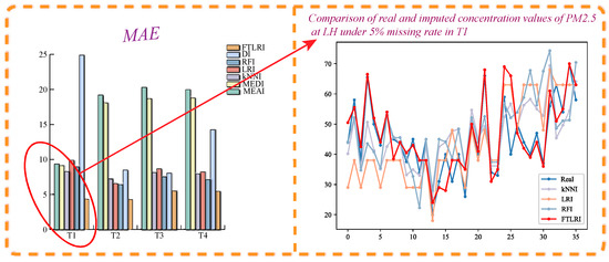
Figure 4. MAE of imputation results of PM_2.5 at LH under 5% missing rate.

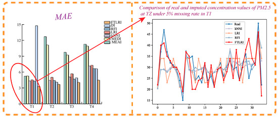
Figure 5. MAE of imputation results of PM_2.5 at YZ under 5% missing rate.

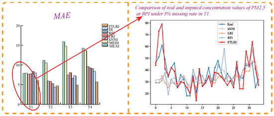
Figure 6. MAE of imputation results of PM_2.5 at BPI under 5% missing rate.

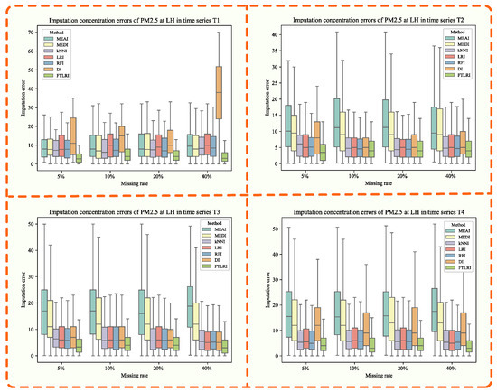
Figure 7. Imputation concentration errors of PM_2.5 generated by MEAI, MEDI, kNNI, LRI, RFI, DI, FTLRI at LH in different time series.

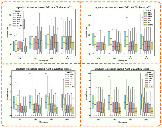
Figure 8. Imputation concentration errors of PM_2.5 generated by MEAI, MEDI, kNNI, LRI, RFI, DI, FTLRI at YZ in different time series.

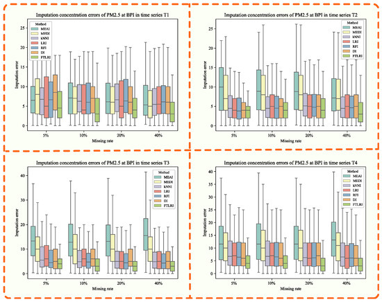
Figure 9. Imputation concentration errors of PM_2.5 generated by MEAI, MEDI, kNNI, LRI, RFI, DI, FTLRI at BPI in different time series.

3.3.1. Imputation of Missing Concentration Values of PM_2.5 at LH

Table 5 shows the quantitative evaluation of the imputation results of PM_2.5 in the short-term time series T1 and T2 and the long-term time series T3 and T4 under different missing rates at LH. When the missing rate was 5%, 10%, 20%, and 40%, respectively, the MAE, MSE, and MAPE of the PM_2.5 imputation results obtained by FTLRI were the lowest compared with the other five classical imputation methods and the new dynamic imputation method using neural networks in both the short-term time series T1 and T2, as well as the long-term time series T3 and T4. The performance of the random forest imputation was slightly worse than that of FTLRI, ranking second among these methods. Mean imputation and Median imputation produced almost the worst results. Dynamic imputation was slightly better than Median imputation and Mean imputation, but its performance was worse than logistic regression. The imputation performance of logistic regression was unstable, and it was worse than that of the k-nearest neighbor imputation on the whole.

To see the performance of FTLRI more visually, Figure 4 clearly depicts a specific imputation effect diagram of PM_2.5 with a missing rate of 5% as an example at LH. The bar chart on the left provides the diagram of the MAE obtained after PM_2.5 was imputed, while the line chart on the right takes short-term time series T1 as an example to describe the values of PM_2.5 imputed by the different imputation methods and the corresponding real values of PM_2.5. For the graph on the right side in Figure 4, the horizontal axis represents the time frames of the missing concentrations of PM_2.5 in time series T1, and the vertical axis represents the concentration values of PM_2.5. Aiming at more clearly showing the imputed values and the true values of PM_2.5 on the right side, we only plotted the imputation results of the four relatively superior-performance methods. As can be seen from the bar chart on the left, the assessment index MAE of the imputation results of FTLRI proposed in this paper was significantly lower than that of the other six imputation methods, in both short-term and long-term time series, which indicates that the performance of FTLRI proposed in this paper is significantly better than that of the other five classical imputation methods and the new dynamic imputation method using a neural network. As can be seen from the line chart on the right, the values imputed by FTLRI were more fitting to the corresponding real values of PM_2.5 than the other four classical methods, which again shows that the imputation performance of the proposed method FTLRI in this paper stays ahead of the other imputation methods from a quantitative point of view.

Aiming at more intuitively comparing the imputation performance of FTLRI with the other five classical imputation approaches and the new dynamic imputation method using a neural network, Figure 7 shows the imputation errors of PM_2.5 at LH in different time series under different missing rates. The imputation errors are expressed as the absolute values of the results calculated by subtracting the values imputed by different methods from the corresponding real value of PM_2.5. The smaller the absolute value is, the smaller the error is, and the better the corresponding imputation methods are. The horizontal coordinate of each subplot indicates the various missing rates, and the vertical coordinate indicates the imputation errors, while the colors represent the corresponding imputation methods. As can be seen from Figure 7, the errors of FTLRI were smaller than that of the other methods, and the median lines of the box plot of FTLRI were also lower than that of the other five classical imputation methods and the new dynamic imputation method using a neural network, which further indicates that FTLRI has an advantage in missing data imputation compared with the other methods under different missing rates in both short-term and long-term time series.

From the above three perspectives, we can draw a conclusion that FTLRI has a big advantage in the missing data imputation at LH under different missing rates, and the imputation performance does not fall with the growing of missing rates and number of data points in the dataset. The cause for that phenomenon is that the imputation results of FTLRI put forward in this paper only depend on the first five and the last three complete data points, which are highly relevant to the data point with missing values in terms of time and attributes. Instead of relying on all the other complete data points, like other imputation approaches, FTLRI selects the eight data points highly correlated with the missing data point to impute the missing value, which is beneficial for imputation performance [46,47]. Therefore, the increasing of the number of data points and the changing of missing rates will not affect the performance of FTLRI, that is, FTLRI can provide superior imputation results on datasets with different missing rates and different numbers of data points.

3.3.2. Imputation of Missing Concentration Values of PM_2.5 at YZ

Table 6 shows the quantitative evaluation of the imputation results of PM_2.5 in the short-term time series T1 and T2 and the long-term time series T3 and T4 under different missing rates at YZ. When the missing rate was 5%, 10%, 20%, and 40%, respectively, the MAE, MSE, and MAPE of the PM_2.5 imputation results obtained by FTLRI were the lowest compared with the other five classical imputation methods and the new dynamic imputation method using neural networks, in both short-term time series T1 and T2, as well as long-term time series T3 and T4, that is, the imputation performance of FTLRI was still superior to the others in both short-term and long-term time series on the whole.

Figure 5 clearly depicts a specific imputation effect diagram of PM_2.5 with a missing rate of 5% as an example at YZ. The bar chart on the left provides the diagram of the MAE obtained after PM_2.5 was imputed, while the line chart on the right takes short-term time series T1 as an example to describe the values of PM_2.5 imputed by the four relatively superior imputation methods and the corresponding real concentration values of PM_2.5. For the graph on the right side in Figure 5, the horizontal axis represents the time frames of the missing concentrations of PM_2.5 in time series T1, and the vertical axis represents the concentration values of PM_2.5. As can be seen from Figure 5, the proposed method FTLRI still achieved better performance than the other five classical imputation methods and the new dynamic imputation method using a neural network.

Figure 8 shows the imputation errors of PM_2.5 generated by MEAI, MEDI, kNNI, LRI, RFI, DI, FTLRI at YZ in different time series under different missing rates. The horizontal coordinate of each subplot indicates the different missing rates, and the vertical coordinate indicates the imputation errors, while the colors represent the corresponding imputation methods. As can be seen from Figure 8, FTLRI still had an advantage in missing data imputation compared with the other five classical methods and the new dynamic imputation method using a neural network under different missing rates in both short-term and long-term time series.

3.3.3. Imputation of Missing Concentration Values of PM_2.5 at BPI

Table 7 shows the quantitative evaluation of the imputation results of PM_2.5 in the short-term time series T1 and T2 and the long-term time series T3 and T4 under different missing rates at BPI. When the missing rate was 5%, 10%, 20%, and 40%, respectively, the MAE, MSE, and MAPE of the PM_2.5 imputation results obtained by FTLRI were almost the lowest compared with the other six imputation methods, in both short-term time series T1 or T2 and long-term time series T3 or T4, that is, the imputation performance of FTLRI was still superior to the others in both short-term and long-term time series on the whole.

Figure 6 clearly depicts a specific imputation effect diagram of PM_2.5 with a missing rate of 5% as an example at BPI. The bar chart on the left provides the diagram of the MAE obtained after PM_2.5 was imputed, while the line chart on the right takes short-term time series T1 as an example to describe the values of PM_2.5 imputed by the four relatively superior imputation methods and the corresponding real values of PM_2.5. As can be seen from Figure 6, the proposed method FTLRI almost achieves better performance than the other six imputation methods at BPI on the whole.

Figure 9 shows the imputation errors of PM_2.5 at BPI in different time series under different missing rates. The horizontal coordinate of each subplot indicates the various missing rates, and the vertical coordinate indicates the imputation errors, while the colors represent the corresponding imputation methods. As can be seen from Figure 9, FTLRI still had an advantage in missing data imputation compared with the other five classical methods and the new dynamic imputation method using a neural network under different missing rates in both short-term and long-term time series at BPI.

Through the exploration of the PM_2.5 imputation results at the above three stations under different missing rates, we can conclude that the imputation method FTLRI put forward in this paper is in a dominant position compared with the other five classical imputation methods and the new dynamic imputation method using a neural network for time series air quality datasets with discrete missing values. Specifically, for low-missing-rate time series air quality datasets with discrete missing values, FTLRI can achieve good imputation performance. Furthermore, for relatively high-missing-rate datasets, FTLRI can also achieve more accurate imputation results by using the extremely related data to the missing data instead of relying on all the other data like other methods.

3.4. Demonstrate the Reasonableness of Choosing the “First Five” Data Points and the “Last Three” Data Points in Step 2

In Step 2 of FTLRI, we searched for the highly relevant data points by selecting the first five data points and the last three data points closest to the missing value in time based on Step 1. In this subsection, we discuss the influence of the specified number of data points closest to the missing value before and after the time on the imputation performance. For convenience, the number of highly correlated data points before the time corresponding to the missing value is represented as prior, and the number of highly correlated data points after the time corresponding to the missing value is represented as rear.

By setting prior and rear from 1 to 10, respectively, to reduce time consumption, we evaluated the corresponding MAE on the benchmark datasets with different missing rates. Figure 10 illustrates the mean values of the MAE of imputation results for all the datasets under different missing rates, and the MAE of imputation results in T3 under a missing rate of 40% at BPI. The stable experimental results in Figure 10 prove that FTLRI is insensitive to prior and rear and indicate that FTLRI is a robust imputation method. Selecting the first five and the last three as a common rule of thumb basically achieved superior imputation performance. In a real application, to access a relatively desired performance, we suggest setting prior and rear from 1 to 10.

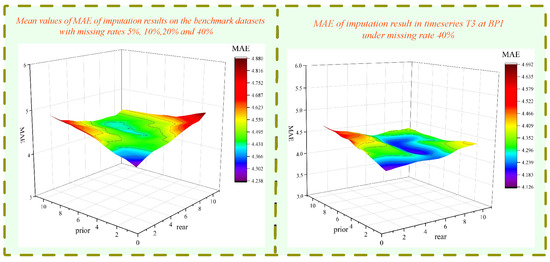
Figure 10. The impact of different priors and rear on FTLRI imputation performance.

4. Conclusions

To accurately fill missing values in a time series air quality dataset, this paper proposes a simple but effective and robust imputation method, called FTLRI. By combining a presented model FT with logistic regression, FTLRI utilizes FT to select the data extremely related to the missing data, both in terms of time and attributes, and applies logistic regression to establish an objective regression equation to obtain the corresponding parameter vector through the selected extremely related data, then employs the parameter vector and other attribute values of the missing data point to obtain the missing value. The limitation with respect to FTLRI is that it fails to impute the missing data points effectively when there are missing values in the eight extremely related data points due to the failure to train an imputation model. In this situation, it is necessary to find another appropriate imputation approach to complete the imputation of missing values. Experiments on the time series air quality data of three different stations in Lanzhou in 2019 have shown that FTLRI can yield more favorable imputation outcomes for both the particular short-term and long-term data under different missing rates. We look forward to applying FTLRI to other time series datasets with discrete missing values, such as share prices and medical monitoring, to verify its validity in the future.

References

- Pang, Y.; Huang, W.; Luo, X.-S.; Chen, Q.; Zhao, Z.; Tang, M.; Hong, Y.; Chen, J.; Li, H. In-vitro human lung cell injuries induced by urban PM2.5 during a severe air pollution episode: Variations associated with particle components. Ecotoxicol. Environ. Saf. 2020, 206, 111406. [Google Scholar] [CrossRef] [PubMed]
- Li, Y.; Myint, S.W. Fine resolution air quality dynamics related to socioeconomic and land use factors in the most polluted desert metropolitan in the American Southwest. Sci. Total Environ. 2021, 788, 147713. [Google Scholar] [CrossRef] [PubMed]
- Zhu, X.; Xia, C. Visual network analysis of the baidu-index data on greenhouse gas. Int. J. Mod. Phys. B 2021, 35, 2150115. [Google Scholar] [CrossRef]
- Kandula, S.; Shaman, J. Reappraising the utility of google flu trends. PLoS Comput. Biol. 2019, 15, e1007258. [Google Scholar] [CrossRef] [PubMed] [Green Version]
- Li, Z.; Wang, D.; Sui, P.; Long, P.; Yan, L.; Wang, X.; Yan, P.; Shen, Y.; Dai, H.; Yang, X.; et al. Effects of different agricultural organic wastes on soil GHG emissions: During a 4-year field measurement in the North China Plain. Waste Manag. 2018, 81, 202–210. [Google Scholar] [CrossRef] [PubMed]
- Wynes, S.; Nicholas, K.A. The climate mitigation gap: Education and government recommendations miss the most effective individual actions. Environ. Res. Lett. 2017, 12, 074024. [Google Scholar] [CrossRef] [Green Version]
- Li, S.-T.; Shue, L.-Y. Data mining to aid policy making in air pollution management. Expert Syst. Appl. 2004, 27, 331–340. [Google Scholar] [CrossRef]
- Picornell, A.; Oteros, J.; Ruiz-Mata, R.; Recio, M.; Trigo, M.M.; Martínez-Bracero, M.; Lara, B.; Serrano-García, A.; Galán, C.; García-Mozo, H.; et al. Methods for interpolating missing data in aerobiological databases. Environ. Res. 2021, 200, 111391. [Google Scholar] [CrossRef]
- Peng, D.; Zou, M.; Liu, C.; Lu, J. RESI: A Region-Splitting Imputation method for different types of missing data. Expert Syst. Appl. 2021, 168, 114425. [Google Scholar] [CrossRef]
- Little, R.J.A.; Rubin, D.B. Statistical Analysis with Missing Data, 2nd ed.; John Wiley & Sons: Hoboken, NJ, USA, 2002. [Google Scholar]
- Maheswari, K.; Priya, P.P.A.; Ramkumar, S.; Arun, M. Missing Data Handling by Mean Imputation Method and Statistical Analysis of Classification Algorithm. In Proceedings of the EAI International Conference on Big Data Innovation for Sustainable Cognitive Computing, Coimbatore, India, 18–19 December 2020; Springer: Berlin/Heidelberg, Germany, 2020; pp. 137–149. [Google Scholar]
- Ispirova, G.; Eftimov, T.; Seljak, B.K. Evaluating missing value imputation methods for food composition databases. Food Chem. Toxicol. 2020, 141, 111368. [Google Scholar] [CrossRef]
- Stead, A.D.; Wheat, P. The case for the use of multiple imputation missing data methods in stochastic frontier analysis with illustration using English local highway data. Eur. J. Oper. Res. 2020, 280, 59–77. [Google Scholar] [CrossRef]
- Pandey, A.K.; Singh, G.; Sayed-Ahmed, N.; Abu-Zinadah, H. Improved estimators for mean estimation in presence of missing information. Alex. Eng. J. 2021, 60, 5977–5990. [Google Scholar] [CrossRef]
- Zainuri, N.A.; Jemain, A.A.; Muda, N. A Comparison of Various Imputation Methods for Missing Values in Air Quality Data. Sains Malays. 2015, 44, 449–456. [Google Scholar] [CrossRef]
- Saeipourdizaj, P.; Sarbakhsh, P.; Gholampour, A. Application of imputation methods for missing values of PM10 and O3 data: Interpolation, moving average and K-nearest neighbor methods. Environ. Health Eng. Manag. 2021, 8, 215–226. [Google Scholar] [CrossRef]
- Schneider, T. Analysis of Incomplete Climate Data: Estimation of Mean Values and Covariance Matrices and Imputation of Missing Values. J. Clim. 2001, 14, 853–871. [Google Scholar] [CrossRef]
- Liu, X.; Wang, X.; Zou, L.; Xia, J.; Pang, W. Spatial imputation for air pollutants data sets via low rank matrix completion algorithm. Environ. Int. 2020, 139, 105713. [Google Scholar] [CrossRef]
- Junninen, H.; Niska, H.; Tuppurainen, K.; Ruuskanen, J.; Kolehmainen, M. Methods for imputation of missing values in air quality data sets. Atmos. Environ. 2004, 38, 2895–2907. [Google Scholar] [CrossRef]
- Davey, A. Statistical Power Analysis with Missing Data: A Structural Equation Modeling Approach; Routledge: London, UK, 2009. [Google Scholar]
- Wilson, D.R.; Martinez, T.R. Improved heterogeneous distance functions. J. Artif. Intell. Res. 1997, 6, 1–34. [Google Scholar] [CrossRef]
- Liaw, A.; Wiener, M. Classification and regression by randomforest. R News 2002, 2, 18–22. [Google Scholar]
- Cheng, C.-H.; Chan, C.P.; Sheu, Y.-J. A novel purity-based k nearest neighbors imputation method and its application in financial distress prediction. Eng. Appl. Artif. Intell. 2019, 81, 283–299. [Google Scholar] [CrossRef]
- Hong, S.; Lynn, H.S. Accuracy of random-forest-based imputation of missing data in the presence of non-normality, non-linearity, and interaction. BMC Med. Res. Methodol. 2020, 20, 199. [Google Scholar] [CrossRef] [PubMed]
- De Freitas, A.G.M.; Minho, L.A.C.; de Magalhães, B.E.A.; Dos Santos, W.N.L.; Santos, L.S.; de Albuquerque Fernandes, S.A. Infrared spectroscopy combined with random forest to determine tylosin residues in powdered milk. Food Chem. 2021, 365, 130477. [Google Scholar] [CrossRef] [PubMed]
- Wang, H.; Yuan, Z.; Chen, Y.; Shen, B.; Wu, A. An industrial missing values processing method based on generating model. Comput. Netw. 2019, 158, 61–68. [Google Scholar] [CrossRef]
- Gómez-Carracedo, M.P.; Andrade, J.M.; López-Mahía, P.; Muniategui, S.; Prada, D. A practical comparison of single and multiple imputation methods to handle complex missing data in air quality datasets. Chemom. Intell. Lab. Syst. 2014, 134, 23–33. [Google Scholar] [CrossRef]
- Han, J.; Pei, J.M. Kamber, Data Mining: Concepts and Techniques; Elsevier: Amsterdam, The Netherlands, 2011. [Google Scholar]
- Ahmadini, A.A.H. A novel technique for parameter estimation in intuitionistic fuzzy logistic regression model. Ain Shams Eng. J. 2021, 13, 101518. [Google Scholar] [CrossRef]
- Dumitrescu, E.; Hué, S.; Hurlin, C.; Tokpavi, S. Machine learning for credit scoring: Improving logistic regression with non-linear decision-tree effects. Eur. J. Oper. Res. 2021, 297, 1178–1192. [Google Scholar] [CrossRef]
- Jiang, F.; Zhidong, G.; Zengshan, L.; Xiaodong, W. A method of predicting visual detectability of low-velocity impact damage in composite structures based on logistic regression model. Chin. J. Aeronaut. 2021, 34, 296–308. [Google Scholar] [CrossRef]
- Waljee, A.K.; Mukherjee, A.; Singal, A.G.; Zhang, Y.; Warren, J.; Balis, U.; Marrero, J.; Zhu, J.; Higgins, P. Comparison of imputation methods for missing laboratory data in medicine. BMJ Open 2013, 3, e002847. [Google Scholar] [CrossRef]
- Zhu, C.; Idemudia, C.U.; Feng, W. Improved logistic regression model for diabetes prediction by integrating PCA and K-means techniques. Inform. Med. Unlocked 2019, 17, 100179. [Google Scholar] [CrossRef]
- Tian, D.; Fan, J.; Jin, H.; Mao, H.; Geng, D.; Hou, S.; Zhang, P.; Zhang, Y. Characteristic and Spatiotemporal Variation of Air Pollution in Northern China Based on Correlation Analysis and Clustering Analysis of Five Air Pollutants. J. Geophys. Res. Atmos. 2020, 125, e2019JD031931. [Google Scholar] [CrossRef]
- Verma, R.; Krishan, K.; Rani, D.; Kumar, A.; Sharma, V.; Shrestha, R.; Kanchan, T. Estimation of sex in forensic examinations using logistic regression and likelihood ratios. Forensic Sci. Int. Rep. 2020, 2, 100118. [Google Scholar] [CrossRef]
- Han, J.; Kang, S. Dynamic imputation for improved training of neural network with missing values. Expert Syst. Appl. 2022, 194. [Google Scholar] [CrossRef]
- Cohen, I.; Huang, Y.; Chen, J.; Benesty, J. Pearson Correlation Coefficient. In Noise Reduction in Speech Processing; Springer: Berlin/Heidelberg, Germany, 2009. [Google Scholar]
- Peng, C.-Y.J.; Lee, K.L.; Ingersoll, G.M. An Introduction to Logistic Regression Analysis and Reporting. J. Educ. Res. 2002, 96, 3–14. [Google Scholar] [CrossRef]
- Fan, Y.; Bai, J.; Lei, X.; Zhang, Y.; Zhang, B.; Li, K.C.; Tan, G. Privacy preserving based logistic regression on big data. J. Netw. Comput. Appl. 2020, 171, 102769. [Google Scholar] [CrossRef]
- Andrychowicz, M.; Denil, M.; Gomez, S.; Hoffman, M.W.; Pfau, D.; Schaul, T.; Shillingford, B.; De Freitas, N. Learning to learn by gradient descent by gradient descent. Adv. Neural Inf. Processing Syst. 2016, 29. [Google Scholar]
- Kelley, C.T. Solving Nonlinear Equations with Newton’s Method; SIAM: Philadelphia, PA, USA, 2003. [Google Scholar] [CrossRef]
- Kabir, G.; Tesfamariam, S.; Hemsing, J.; Sadiq, R. Handling incomplete and missing data in water network database using imputation methods. Sustain. Resilient Infrastruct. 2020, 5, 365–377. [Google Scholar] [CrossRef]
- Niu, M.; Sun, S.; Wu, J.; Yu, L.; Wang, J. An innovative integrated model using the singular spectrum analysis and nonlinear multi-layer perceptron network optimized by hybrid intelligent algorithm for short-term load forecasting. Appl. Math. Model. 2016, 40, 4079–4093. [Google Scholar] [CrossRef]
- Hka, N.D.; Tahir, N.M.; Abd Latiff, Z.I.; Jusoh, M.H.; Akimasa, Y. Missing data imputation of MAGDAS-9’s ground electromagnetism with supervised machine learning and conventional statistical analysis models. Alex. Eng. J. 2022, 61, 937–947. [Google Scholar] [CrossRef]
- Gomišček, B.; Hauck, H.; Stopper, S.; Preining, O. Preining, Spatial and temporal variations of PM1, PM2.5, PM10 and particle number concentration during the auphep—Project. Atmos. Environ. 2004, 38, 3917–3934. [Google Scholar] [CrossRef]
- Audigier, V.; Husson, F.; Josse, J. A principal component method to impute missing values for mixed data. Adv. Data Anal. Classif. 2016, 10, 5–26. [Google Scholar] [CrossRef]
- Hasan, M.K.; Alam, M.A.; Roy, S.; Dutta, A.; Jawad, M.T.; Das, S. Missing value imputation affects the performance of machine learning: A review and analysis of the literature (2010–2021). Inform. Med. Unlocked 2021, 27, 100799. [Google Scholar] [CrossRef]
Publisher’s Note: MDPI stays neutral with regard to jurisdictional claims in published maps and institutional affiliations. |
© 2022 by the authors. Licensee MDPI, Basel, Switzerland. This article is an open access article distributed under the terms and conditions of the Creative Commons Attribution (CC BY) license (https://creativecommons.org/licenses/by/4.0/).