Improving the Performance of Pipeline Leak Detection Algorithms for the Mobile Monitoring of Methane Leaks

Abstract

Methane (CH₄) is the major component of natural gas, a potent greenhouse gas, and a precursor for the formation of tropospheric ozone. Sizable CH₄ releases can occur during gas extraction, distribution, and use, thus, the detection and the control of leaks can help to reduce emissions. This study develops, refines, and tests algorithms for detecting CH₄ peaks and estimating the background levels of CH₄ using mobile monitoring, an approach that has been used to determine the location and the magnitude of pipeline leaks in a number of cities. The algorithm uses four passes of the data to provide initial and refined estimates of baseline levels, peak excursions above baseline, peak locations, peak start and stop times, and indicators of potential issues, such as a baseline shift. Peaks that are adjacent in time or in space are merged using explicit criteria. The algorithm is refined and tested using 1-s near-ground CH₄ measurements collected on 20 days while driving about 1100 km on surface streets in Detroit, Michigan by the Michigan Pollution Assessment Laboratory (MPAL). Sensitivity and other analyses are used to evaluate the effects of each parameter and to recommend a parameter set for general applications. The new algorithm improves the baseline estimates, increases sensitivity, and more consistently merges nearby peaks. Comparisons of two data subsets show that results are repeatable and reliable. In the field study application, we detected 534 distinct CH₄ peaks, equivalent to ~0.5 peaks per km traveled; larger peaks detected at nine locations on multiple occasions suggested sizable pipeline leaks or possibly other CH₄ sources.

1. Introduction

1.1. Significance of Methane Leaks from Natural Gas Infrastructure

Atmospheric concentrations of methane (CH₄) have risen at a rate of 0.5% per year over the past decade [1], and this gas now causes the largest radiative forcing (0.97 W/m²) after CO₂ [2,3]. The largest anthropogenic sources of CH₄ are agriculture and waste management activities, followed by the fossil fuel industry, which emitted ~33% of the global total in 2000–2009 and over 40% of the U.S. total [4]. Increased natural gas supplies, due to enhanced recovery techniques, such as hydraulic fracturing and horizontal drilling, have tremendously increased the share of natural gas used to generate electrical power in the U.S. [5]. At the same time, fugitive releases from leaks during natural gas extraction, distribution, and application are likely to experience a great increase. Notably, much of the gas transmission and distribution system, especially mains and service lines in cities, is old and prone to leaks, and recent reports suggest significant underreporting of pipeline CH₄ leaks [6,7]. Older studies report many events likely to release CH₄, e.g., 959 transmission line incidents in 2002–2009 and 823 distribution line incidents in 2004–2009 in the U.S. [8]. A vastly higher number of leaks likely occurs from mains and service lines, e.g., extrapolations of field studies in 12 cities suggest that some 630,000 leaks in U.S. distribution mains emit 0.69 Tg/year of CH₄ [7]. The detection and the repair of pipeline leaks remains important for safety, economic, and environmental reasons. Unfortunately, traditional leak detection approaches have many shortcomings.

1.2. Leak Detection Methods

Conventional leak detection methods for natural gas pipelines include acoustic methods, gas sampling and analysis, and soil monitoring. Acoustic methods detect the sound generated by escaping gas. While simple, these methods cannot detect small leaks if faint sounds are obscured by background noise [9]. Gas sampling methods typically use hand-held detectors, such as flame ionization detectors (FIDs) and sampling probes to measure gas concentrations along a sampling route. While small leaks can be detected, the process is slow and the sampling area is small and limited by the probe [9]. In soil monitoring, a tracer gas, such as SF₆ or CO₂, is injected into a buried gas pipeline and monitored in air just above the soil surface [10]. While potentially accurate and sensitive, this method is expensive since the tracer must be continuously added [11]. In addition, all of these methods require staff to patrol the pipeline with hand-held instruments, which is labor-intensive, difficult to ensure full spatial coverage of large and complex urban distribution systems, and prone to both false positives and false negatives. Very large leaks can be detected using volume or mass balance methods, which compare the volume of gas entering and exiting a pipeline section [12]. While inexpensive, these methods cannot detect small leaks, and they do not indicate leak locations [11]. Other leak detection methods use real-time modeling, negative pressure wave, and pressure point analyses [11,13].

In recent years, CH₄ leaks have been detected using mobile monitoring and sensitive, selective and fast-response instrumentation, including cavity ring-down spectroscopy [14], tunable diode laser absorption spectroscopy (TDLAS) [15], laser induced fluorescence (LIF) [16,17], Fourier transform infrared spectroscopy (FTIR) [18], and thermal imaging [9,11]. These instruments remain too large, heavy, expensive, and power hungry to be carried by staff or to be permanently installed along pipelines. Similar portable instruments such as Remote Methane Leak Detector (RMLD) and portable cavity ringdown spectroscopy sensors from Picarro are commercially available, but these methods are highly labor-intensive and cannot fully cover complex distribution systems in cities. However, installed on mobile platforms, such as vehicles and airplanes, gas leaks are easily detected, e.g., in 2-month campaigns, a vehicle-based system using a cavity ring-down spectrometer detected 3356 CH₄ leaks in Boston, Massachusetts and 5893 leaks in Washington, DC [19]. The δ¹³C-isotopic signature indicated that the elevated CH₄ levels had a fossil fuel, rather than a biogenetic, source. Such instruments installed in Google Street View cars have detected thousands of leaks in 15 U.S. cities [6,20], using an open-source algorithm [21]. Even more recently, drone-based platforms using laser spectrometry to detect CH₄ leaks also are being developed [22,23,24]. Mobile monitoring has also been used in estimating on-road traffic emissions and related recent publications reported novel methods and algorithms to separate peak and background concentrations [25,26].

1.3. Study Objectives

Our overall goals are to assess and to enhance the ability to reliably determine the location and the magnitude of subsurface natural gas pipeline leaks using mobile monitoring. Here we focus on the algorithms for estimating background, peak levels, and peak locations. We use field data collected by the Michigan Pollution Assessment Laboratory (MPAL), a mobile laboratory equipped with two sensitive CH₄ instruments, and utilize two 10-day subsets of near-ground CH₄ data and other information collected in a portion of Detroit, Michigan. The study site is diverse, and it includes residential, commercial, and industrial areas, as well as a mix of new and old infrastructure. We conduct a sensitivity analysis on key parameters in the algorithm, compare results with other published methods, examine the repeatability of results, and recommend a parameter set for general use.

2. Methods

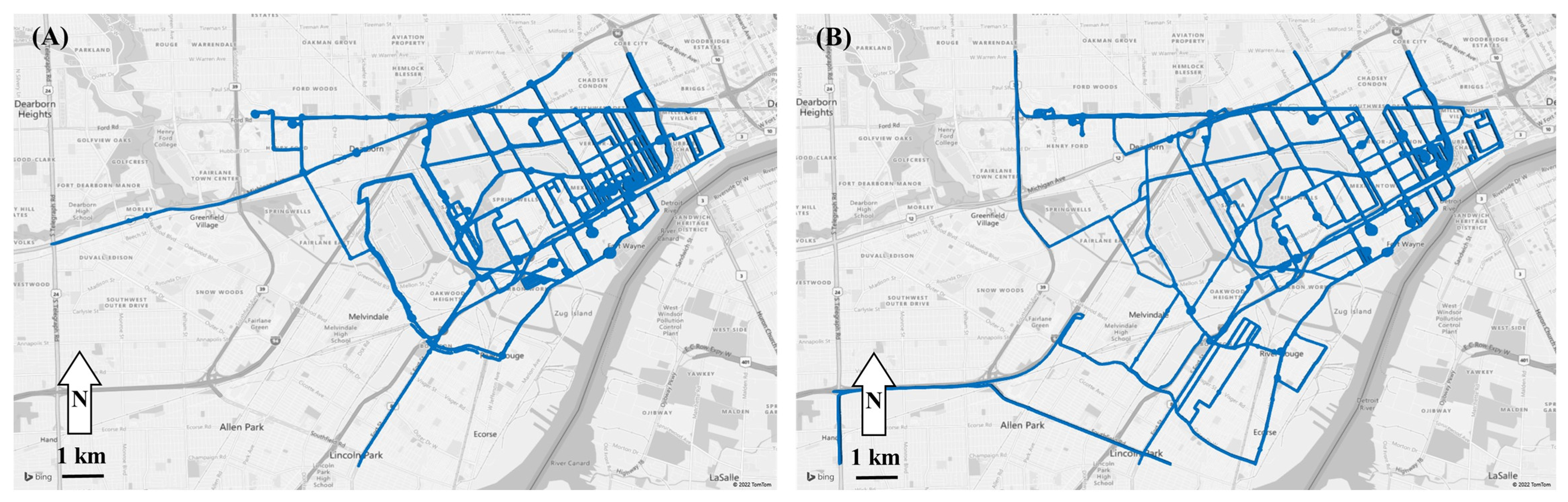
2.1. Study Site and Sampling Schedule

Measurements were collected in a 17 × 10 km portion of Detroit, Michigan from 19 May 2021, to 15 December 2021, as a part of the Michigan–Ontario Ozone Source Experiment (MOOSE) project. We use two data subsets to test and refine the peak detection and characterization algorithm. The first subset was collected on 10 days (26/May/2021, 2/Jun/2021, 7/Jun/2021, 20/Sep/2021, 22/Oct/2021, 27/Oct/2021, 3/Nov/2021, 4/Nov/2021, 12/Nov/2021, 17/Nov/2021) and used to develop and refine the algorithm. A second data subset, also using 10 days (27/May/2021, 11/Jun/2021, 15/Jun/2021, 7/Jul/2021, 23/Aug/2021, 14/Sep/2021, 24/Sep/2021, 8/Oct/2021, 13/Oct/2021, 10/Nov/2021), evaluated the performance and the repeatability of the algorithm. Dates, meteorology conditions based on observations at four local airport stations (Detroit Metro Wayne County Airport (DTW), Grosse Ile Municipal Airport, Detroit City Airport, Willow Run Airport) reporting to the National Weather Service, and sampling schedules are summarized in

Table 1. Summary of sampling schedule (in local time, EST) and meteorological conditions of the 20 days in the two data subsets. Meteorological variables represent the average (circular average for wind direction and scalar average for the rest parameters) for the study period derived from data from four local airports (measured at 10 m).

Date	Time_Start	Time_End	Temperature (°C)	Wind_Direction (deg)	Wind_Speed (m/s)	Ceiling_Height (m)	Pressure (mbar)
Data Subset 1
26/May/2021	14:30	18:30	23.8	269	5.6	11,971	1013.8
2/Jun/2021	9:30	12:00	19.0	181	2.9	1966	1018.8
7/Jun/2021	11:00	15:30	27.1	189	4.8	11,061	1015.3
20/Sep/2021	11:00	13:30	26.5	161	4.4	16,421	1017.6
22/Oct/2021	10:00	15:00	10.3	358	2.5	12,405	1017.1
27/Oct/2021	12:00	17:00	11.4	16	1.4	285	1015.9
3/Nov/2021	15:00	18:00	5.9	298	1.0	4804	1027.3
4/Nov/2021	14:00	16:30	6.8	311	2.3	3641	1026.2
12/Nov/2021	10:30	16:00	10.1	220	8.5	10,980	1007.3
17/Nov/2021	11:30	17:30	16.6	209	7.3	560	1009.6
Data Subset 2
27/May/2021	14:00	16:00	18.2	57	5.6	17,973	1019.7
11/Jun/2021	7:30	9:00	25.4	82	2.8	22,000	1010.9
15/Jun/2021	10:00	12:00	23.3	345	5.5	15,140	1016.0
7/Jul/2021	12:00	15:30	28.6	233	4.3	13,373	1011.7
23/Aug/2021	13:00	17:30	29.7	293	3.1	22,000	1013.7
14/Sep/2021	10:30	15:00	29.7	214	7.3	14,513	1009.2
24/Sep/2021	9:00	12:00	19.0	256	5.2	19,281	1014.9
8/Oct/2021	12:30	16:30	22.7	140	3.2	7106	1016.0
13/Oct/2021	12:00	17:00	22.5	221	3.9	13,649	1014.8
10/Nov/2021	15:00	18:00	10.2	88	2.3	15,679	1022.1

.

2.2. Measurements and Quality Assurance

Data were collected using the Michigan Pollution Assessment Laboratory (MPAL), a truck-based platform that contains five lab-quality instruments to measure gaseous pollutants, five instruments for particulate matter (PM), meteorological sensors, a geographical positioning sensor (GPS), and forward and reverse cameras. All data were collected by MPAL’s data system at 1 Hz. MPAL’s sampling systems, performance evaluations, and quality assurance protocols have been detailed elsewhere [27]. In 2021, MPAL was temporarily adapted into a slightly smaller vehicle without the PM instruments; otherwise, instruments, power, and data acquisition systems were identical. Two sampling inlets were installed: a roof inlet at ~2.5 m height and a front inlet at ~10 cm height above the road, using an array of six vertical, downward-facing sampling ports evenly distributed across the front bumper. Purge flows minimized residence and lag times in the sampling system. Samples were introduced to each instrument following a water trap and 1 µm Teflon filter; the front inlet also used a small splash guard around each port and an additional particle filter to reduce contamination of the Teflon tubing.

CH₄ was measured using two cavity ring-down spectrometers (G2204 and G2401, Picarro, Santa Clara, CA, USA) that have a 0–100 ppm range, 0.001 ppm resolution, and 2 s resolution. Before MOOSE, the two instruments installed on MPAL collected data between March 2019 and March 2020, and they showed accurate and comparable results (e.g., the two instruments had average CH₄ concentrations of 2.05 ± 0.30 ppm and 2.06 ± 0.50 ppm, respectively) [27]. This study focusses on the near-ground data collected by the G2204, which was connected to the front inlet. In addition to measuring CH₄, this instrument also measures H₂S and H₂O.

MPAL incorporated a high-speed GPS (Garmin 18×, Garmin International Inc., Olathe, KS, USA) that measured location at 1 Hz with an uncertainty generally under 3 m. An onboard meteorological system measured wind speed and direction (Model 92000, R.M. Young Company, Traverse City, MI, USA); these measurements were corrected for vehicle speed and direction. We supplemented the on-board meteorological data, which could be affected by the relatively low measurement height (~2.5 m), rapid speed, and direction changes of MPAL, as well as other vehicles, trees, and buildings, with meteorological data from four local airports noted earlier, calculating hourly averages of temperature, dew point, wind direction, windspeed, precipitation, ambient pressure, ceiling height, and visibility [28].

Quality assurance checks regularly performed included zero and span checks, and determinations whether sample flows, temperatures, sampling and reactor pressures, and concentration readings were in acceptable ranges. We accounted for the lag time due to instrument response and the sampling inlet system.

2.3. Data Analysis

2.3.1. Initial Data Processing

Data were collected by MPAL’s data acquisition system at 1 Hz, which means 1-s data were logged regardless of the actual instrument resolution. 1-s, 5-s, or 60-s averaged data were consolidated into a master dataset containing CH₄ measurements, time and date, vehicle position and speed, wind speed and direction, and other data. Details on the preliminary data validation and consolidation can be found elsewhere [27].

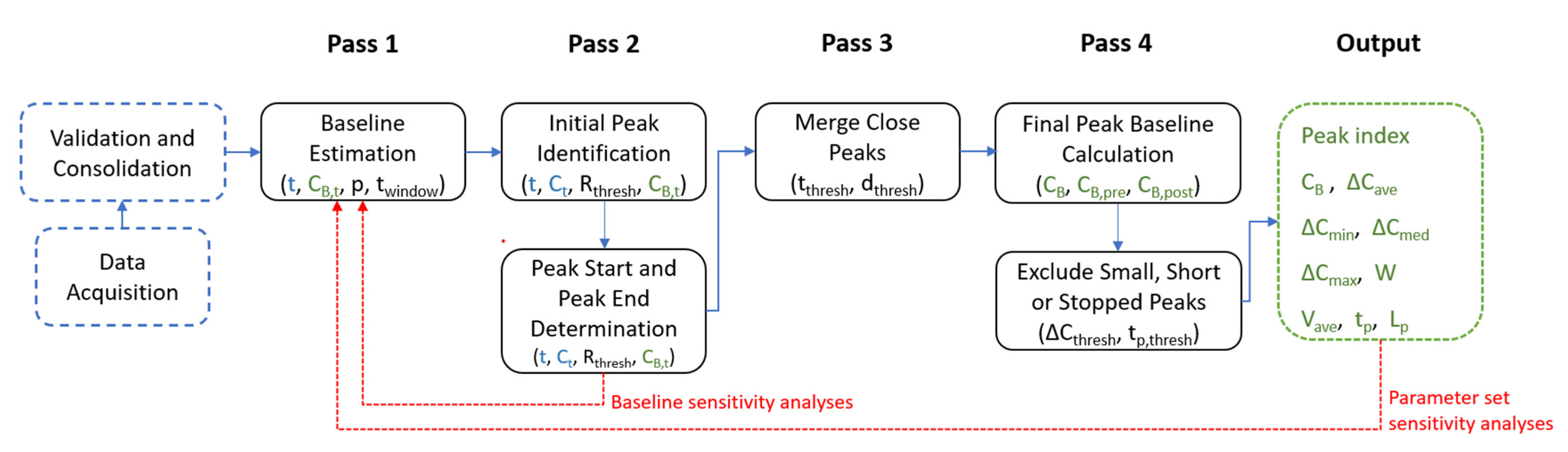
2.3.2. Baseline and Peak Detection Algorithm

An algorithm was developed to identify CH₄ concentration excursions or “peak events” that potentially correspond to pipeline leaks. The algorithm used 1-s data (to provide the greatest resolution) and made four passes of the data (Figure 1). Pass 1 provides initial estimates of baseline levels, which are used in Pass 2 to determine peaks, peak start and stop times, and locations. A peak index is also assigned. Pass 3 merges adjacent peaks, including those close in space and/or time. Pass 4 filters out small or short peaks and refines the baseline. The final output provides peak concentration, average concentration, baseline, start and end times and locations, peak duration, and other statistics, providing a compact representation derived from hundreds of thousands of observations collected in a typical day’s run.

Pass 1 provides local estimates of background concentrations of CH₄, which can differ from the global and the urban average CH₄ concentration (nominally ~2 ppm). Background levels can change slightly in space and in time (generally less than ±0.2 ppm) due to local and to regional emission sources, meteorological effects, and instrumental drift. The initial estimate of baseline concentration at time t, C_B,t (ppm), is calculated as percentile p of measurements within a time window that extended t_window seconds both before and after the present time. The selection of the percentile and the time window jointly affect the baseline and the bias that might occur if peaks occur in or near the time window. We evaluated percentiles p from 1 to 50% and time windows t_window from 100 to 600 s. Baseline levels (and peaks) were not estimated if data gaps in the time window exceeded 30 s. This initial baseline estimate is subsequently refined in Pass 4.

Pass 2 identifies elevated measurements if the concentration at time t, C_t, exceeds R_thresh × C_B,t, where R_thresh is the ratio of the current concentration to the background concentration needed to identify a peak. We tested R_thresh over a range from 1.015 to 1.1. Lower ratios can detect small peaks, but noise may lead to false positives, while higher ratios reduce these errors but may miss peaks and thus yield false negatives. Using samples collected near the road surface, Weller et al. [21] set R_thresh = 1.1, equivalent to ~0.2 ppm increment over baseline. Pass 2 also determines the start time when the CH₄ level first exceeds R_thresh × C_B,t, and the end time when levels next fall below this concentration. Detected peaks are numbered chronologically.

Pass 3 merges adjacent peaks that are close in space or in time. The time and the distance gaps between adjacent peaks are calculated using the start and the end times and locations (latitude and longitude) for peaks identified in Pass 2, and then adjacent peaks are merged if the time or the distance gap is smaller than predetermined thresholds. We evaluated time gap thresholds, t_thresh (s), from 2 to 10 s, and distance gap thresholds, d_thresh (m), from 10 to 75 m. After merging, new peak numbers are assigned.

Finally, Pass 4 refines the baseline and filters out small or short peaks. The final baseline C_B is calculated as the average of pre- and post-peak baselines, where C_B,pre and C_B,post are the p^th percentile of readings within t_window seconds before the start of the peak, and after the end of the peak, respectively. Thus, this final baseline accounts for possible shifts in baseline, while excluding the peak itself. The maximum concentration of each peak above final baseline, ΔC_max, is calculated. Small peaks that are likely instrument noise are removed if their increments above baseline C_B are smaller than threshold concentration ΔC_thresh (ppm), or if the peak duration is less than the time threshold t_p,thresh (s). To minimize false negatives, small values of ΔC_,thresh and t_p,thresh may be preferred. In addition, Pass 4 filtered out peaks that occurred when the vehicle was stopped for a relatively long time, which can result in long duration peaks and inaccurate baseline estimates; in addition, measurements collected while moving or being stationary may differ due to differences in turbulence and mixing induced by the vehicle as compared to being at rest. We omitted peaks if at least 50% of the peak occurred when the vehicle was stopped, which was determined if the GPS-derived speed was below 0.05 m/s. (When the vehicle is stopped, GPS noise can produce a low velocity.) The final peak numbers were assigned after these steps.

Outputs calculated and archived for each peak included start and end times, start and end locations, baseline concentration C_B, concentration increments above baseline for the peak average, minimum, median, and maximum, ΔC_ave, ΔC_min, ΔC_med, and ΔC_max (ppm), respectively. We also calculated the peak width W (m) as the distance between the peak start and end locations (m), the average driving speed V_ave (m/s) as the peak width divided by its duration t_p (s), and the peak centroid L_p (latitude and longitude vector) as the concentration-weighted spatial average of 1-s measurements during the peak event:

$${\mathrm{L}}_{\mathrm{p}}=\frac{{{\displaystyle \sum }}_{\mathrm{t}=1}^{\mathrm{Np}} ({\mathrm{C}}_{\mathrm{t} }-{ \mathrm{C}}_{\mathrm{B}}){ \mathrm{V}}_{\mathrm{t}\ast }{ \mathrm{l}}_{\mathrm{t}} }{{{\displaystyle \sum }}_{\mathrm{t}=1}^{\mathrm{Np}} ({\mathrm{C}}_{\mathrm{t} }-{ \mathrm{C}}_{\mathrm{B}}){ \mathrm{V}}_{\mathrm{t}\ast } }$$

(1)

where l_t = location (latitude and longitude) at time t, C_t = measured concentration at time t, N_p = number of measurements in the peak event (equivalent to duration in seconds since 1-s data are analyzed), and V_t is the distance traveled during the measurement (m) at time t, or equivalently and more conveniently the vehicle speed (m/s) since 1-s measurements are used. This approach is not optimal if the vehicle stops at some point during the peak event since V_t = 0 and the corresponding CH₄ measurements will not be used, although these measurements could reduce the uncertainty and thus improve the result. To correct this, during stopped periods we define V_t* = V_ave*/N_s where V_ave* = mean speed when the vehicle is moving during the peak event (m/s) and N_s = number of measurements when the vehicle is stopped. In effect, this averages concentrations over the stopped period, producing a data point equivalent in weight to the average measurement during the peak event when the vehicle is moving. Equation (1) provides an appropriate weight for a single stop during a peak event. In the rare event of multiple (separated) stops, an alternative formulation would be required to obtain comparable weights.

2.3.3. Sensitivity Analysis

The algorithm used seven primary parameters: three parameters (p, t_window, R_thresh) determine baselines and peaks in Passes 1 and 2, and four additional parameters (t_thresh, d_thresh, t_p,thresh, ΔC_thresh) merge adjacent peaks and filter out potentially false peaks in Passes 3 and 4. We evaluated these parameters in sensitivity analyses that systematically changed parameter values while recording the number of peaks reported, flagged by predetermined criteria (described below), merged, or filtered out. Additional parameters (Pass 1 baseline skip gap, set as 30 s; Pass 4 filtration criteria due to vehicle stop, set as 50% of measurements; and Pass 4 vehicle stationary speed limit, set as 0.05 m/s) generally had much smaller effects on results. The sensitivity analysis was performed using data subset 1. The selected parameters were then applied to data subset 2.

We tested 100 combinations of the three parameters affecting baseline estimates (full factorial design with p set to 0.01, 0.05, 0.15, 0.25, and 0.50; t_window set to 100, 150, 300, 450, and 600 s, and R_thresh set to 1.015, 1.025, 1.05, and 1.1), and we calculated outputs by setting the four parameters in Passes 3 and 4 at nominal values (t_thresh = 5 s, d_thresh = 10 m, t_p,thresh = 5 s, and ΔC_thresh = 0.03 ppm). These nominal values worked well based on an extensive set of prior tests. The results of each combination was evaluated using heatmaps and other displays for four criteria: number of peaks detected; baseline out of range (i.e., not within 1.8–2.2 ppm); consistently elevated observations in the baseline window (>50% of data in the baseline window); and large baseline shifts (|C_B,pre − C_B,post| > 0.02 ppm). The three latter criteria can identify potentially problematic baseline estimates. From this analysis, a subset of parameter combinations was selected for further analysis. Results were also evaluated using several additional criteria, including the number of small peaks (ΔC_max < 0.1 ppm), long duration peaks (t_p > 240 s), very wide peaks (W > 500 m), and peaks with stopped periods (V_i < 0.05 m/s exceeding 1 s during the peak). We also plotted and inspected concentration and location trends for all peaks. Graphical examples of peaks flagged by the abovementioned seven criteria can be found in Figure S1.

We tested 25 combinations of the parameters used to merge peaks in Pass 3 (setting t_thresh to 2, 3, 5, 7, and 10 s) and d_thresh set to 10, 20, 30, 50, and 75 m), and we examined the number of peaks merged. In this analysis, we fixed the other parameter to nominal values (p = 0.05, t_window = 450 s, R_thresh = 1.05, t_p,thresh = 5 s and ΔC_thresh = 0.03 ppm).

Finally, to test peak filtering in Pass 4, 8 combinations of t_p,thresh (5 and 10 s) and ΔC_thresh (0.02, 0.025, 0.03, and 0.05 ppm) were evaluated and the number of peaks filtered out was determined. Again, other parameters were set to nominal values (p = 0.05, t_window = 450 s, R_th = 1.05, t_thresh = 5 s, and d_thresh = 10 m). These sensitivity analyses demonstrated the interaction between parameters and allowed some “fine tuning” of the approach.

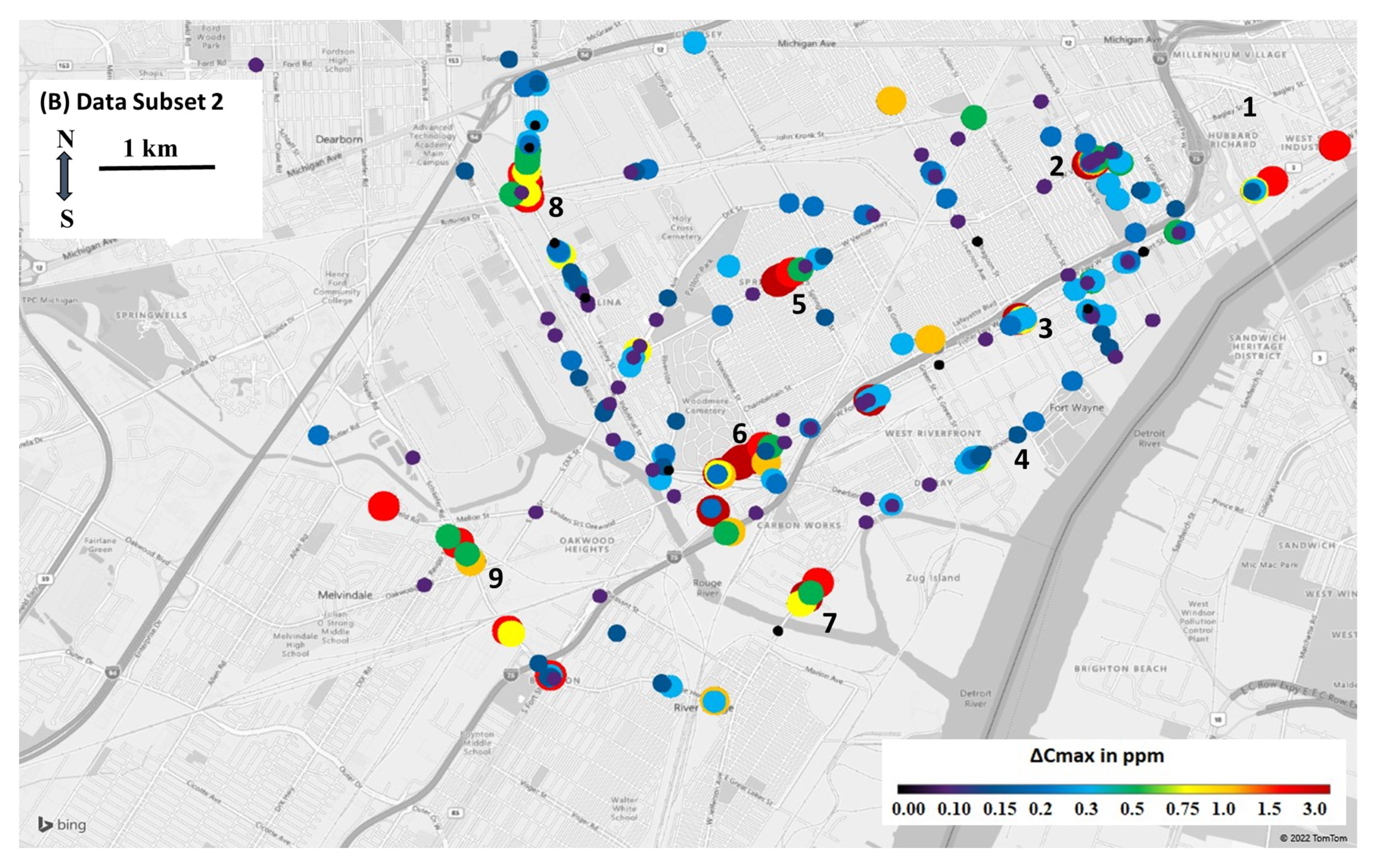
2.3.4. Data Mapping and Visualization

To visualize peaks and baseline levels, we generated “hotspot” maps, which displayed ΔC_max in concentration bins (10 cut-points of 0, 0.10, 0.15, 0.20, 0.30, 0.50, 0.75, 1.00, 1.50, >3.00 ppm); maps of C_B used 7 cut-points (1.85, 1.90, 1.95, 2.00, 2.05, 2.10, >2.15 ppm). These nonlinear bins better display results than linear ranges or bins.

2.3.5. Comparison to Other Peak Detection Algorithms

Results of the new algorithm were compared to the procedure of Weller et al. [21], which had a number of similarities, but set p = 0.5 (median), t_window = 150 s, R_thresh = 1.1, and for adjacent peak merging, t_thresh = 5 s. Weller et al. [21] did not apply a distance gap threshold for peak merging. The two approaches were compared by contrasting peak statistics, probability plots, and scatter plots that matched peaks detected by the different algorithms, using the timestamp of the maximum concentration. We also evaluated trend plots for each peak.

A much simpler, quicker algorithm, using a fixed baseline, was also tested. This was evaluated using three sets of parameters (C_B = 1.9 ppm and R_thresh = 1.1; C_B = 2.0 ppm and R_thresh = 1.05; C_B = 2.2 ppm and R_thresh = 1.025) and the same performance evaluation described above. The evaluations used data subset 1.

3. Results and Discussion

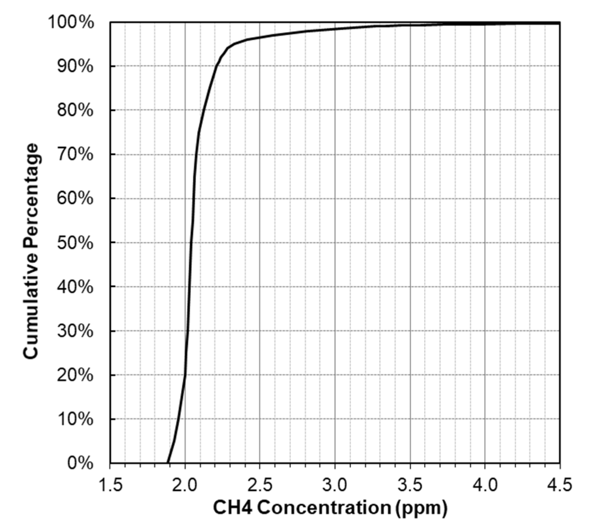
3.1. Data Summary

Data subset 1 contained 10 days of data and a total of 125,025 1-s CH₄ measurements collected in southwest Detroit over a distance of 541 km, while driving at an average speed of 15.6 km/h (Figure 2a). Both median and average measurements of CH₄ (2.04 and 2.10 ppm, respectively) were slightly above the 2021 global average of 1.9 ppm [1]. The skewness of the far right tail of the CH₄ concentration distributions is seen in the probability plot (Figure 3): 1-s levels ranged from 1.88 ppm to 25.5 ppm, and 90th, 98th, 99th, and 99.9th percentile concentrations were 2.21, 2.82, 3.27, and 7.51 ppm, respectively.

3.2. Sensitivity Analyses

3.2.1. Baseline and Initial Peak Finding

Tests using the 100 parameter combinations in Passes 1 and 2 detected from 178 to 589 peaks, depending on the parameter set. Heat maps (Figure S2a) show the influence of t_window, p and R_th. Results were most sensitive to R_thresh (ratio multiplying the background concentration that sets the floor for peak detection), e.g., the number of peaks decreased from 584 to 224 as R_thresh increased from 1.015 to 1.100 (for t_window = 100 s and p = 0.05). As expected, higher R_thresh eliminated small peaks, some of which may be instrument noise or random variability. Results were moderately sensitive to t_window (baseline window width), e.g., the number of peaks gradually decreased from 584 to 417 as t_window lengthened from 100 to 600 s (for R_thesh = 1.015 and p = 0.05). This trend reflects greater chances of data gaps with long windows (since baselines and peaks were not calculated if a data gap exceeding 30 s was detected) and that the data gap would force exclusion of peaks.

Baseline estimates and peak finding were largely insensitive to values of p below 0.25 (percentile used to calculate the baseline concentration), e.g., the number of detected peaks decreased from 588 to 570 as p increased from 0.01 to 0.25 (for t_window = 100 s and R_thresh = 1.015; Figure S2a). At high values, e.g., p = 0.5 (median), however, the number of peaks detected and other criteria were affected, particularly for short time windows. The use of small p (e.g., 0.01) may be preferred since the baseline estimate would effectively exclude elevated measurements, potentially increasing the accuracy of the baseline estimate. Corroborating evidence was seen as decreasing p lowered the out-of-range baseline percentage, e.g., for the 20 t_window and R_thresh combinations, out-of-range baselines were lowered from 9–28% with p = 0.50 to 0–4% with p = 0.01. This also lowered the number of large baseline shifts, e.g., from 46–71% for p = 0.5 to 13–44% for p = 0.01. However, smaller p flagged more peaks with >50% elevated observations in the baseline window (percentage increased from 0–4% to 3–40%) (Figure S2c) since smaller p decreases C_B,t and thus decreases R_thresh × C_B,t. As a result, more measurements were marked as elevated with unchanged t_window and R_thresh. The main issue in using small p, however, is potential sensitivity to instrument noise, e.g., for p = 0.01, C_B is the third lowest 1-s concentration measurement in a 300 s window. While potentially a minor issue for low noise and stable instruments, to improve robustness we recommended setting p to exclude at least the several very lowest measurements in the calculation window.

While the baseline concentration C_B is primarily determined by t_window and p, the presence of peaks in the baseline calculation window can be important. Concentration ratio R_thresh is the key parameter determining both peak finding and the start and the end of peaks. In turn, peak width can affect the final baseline estimate (determined as the average of C_B,pre and C_B,post calculated in Pass 4). Interactions between R_thresh, t_window, and p are depicted in heat maps (Figure S2b–e). Across the 100 parameter combinations, 0 to 28% of peaks were out of baseline range, 0 to 40% of peaks had elevated observations in the baseline window, and 13 to 71% had a baseline shift, possibly due to the low threshold value (|C_B,pre − C_B,post| < 0.02 ppm) used. Generally fewer peaks were flagged with these issues as t_window increased since longer windows diminished the effect of peaks and tended to stabilize the background estimate.

As expected, peak finding was very sensitive to R_thresh (threshold concentration ratio) and considerably fewer peaks were detected or flagged as this parameter increased (Figure S2a,c). Surprisingly, baseline shift increased with R_thresh (Figure S2d), probably since large R_thresh leave out more (slightly) elevated measurements in the baseline calculation window. This may not have much significance for the larger peaks detected with high values of R_thresh; again, it reflects the interaction of these parameters on baseline estimates.

In summary, this analysis suggests several general trends. First, longer windows t_window can improve the baseline estimates although some peaks may be lost due to data gaps in very long windows. In addition, very long windows may not handle situations where large baseline shifts occur over small distances, possibly around area sources such as gas extraction and processing facilities. We did not encounter such situations; these may be atypical in urban settings. Second, values of baseline percentile p below 0.25 had little effect on peak finding. Importantly, the use of a low percentile value (e.g., p from 0.05–0.15) is far preferable to an average or a median, which can be unduly influenced by peaks. Third, while a larger threshold ratio R_thresh can filter out false positives, it also removes true small peaks and affects pre- and post-peak baseline estimates. Our analysis suggests that the best performing parameter set used a middle range for t_window (150–450 s) and R_thresh (1.025–1.05) and a low value for p (0.05). The combination of t_window = 450 s, R_thresh = 1.05, and p = 0.05 had the lowest overall flagged peak percentages (Figure S2e), and it was thus selected as “parameter set 1”, our first option.

Table 2. Selected parameter sets and corresponding algorithm results obtained using data subset 1. The rows show results for different parameter sets including the algorithm published by Weller et al. [21]; sets 1 to 4 highlight selected results from the sensitivity analyses; set 4 results using data subset 2; and fixed baselines of 1.9, 2.0 and 2.2 ppm. The table includes the number of peaks detected after each pass of the algorithm, the percentage of peaks flagged with potential issues, and baseline and peak maximum statistics. Bolded data represents peak finding results with the final selected parameter set.

Parameter Set	Weller et al. [21]	Set 1	Set 2	Set 3	Set 4	Set 4 Data Subset 2	Fixed_BL_1.9	Fixed_BL_2.0	Fixed_BL_2.2
twindow (s)	150	450	450	300	150	150
Rthresh	1.1	1.05	1.025	1.05	1.05	1.05	1.1	1.05	1.025
p	0.50	0.05	0.05	0.05	0.05	0.05
tthresh (s)	5	5	5	5	5	5	5	5	5
dthresh (m)		10	10	10	10	10	10	10	10
ΔCthresh (ppm)	0.03	0.03	0.03	0.03	0.03	0.03	0.03	0.03	0.03
tp,thresh (s)	5	5	5	5	5	5	5	5	5
Peak #_Pass2	206	319	386	337	350	348	309	304	245
Peak #_Pass3	197	277	324	296	305	278	257	254	206
Peak #_Pass4	166	254	246	273	280	254	231	232	184
Flag: BL (start) out of Range (percentage)	16.3%	0.0%	0.0%	0.4%	1.1%	0.0%
Flag: Elevated Obs (percentage)	0.6%	0.8%	16.7%	1.5%	4.3%	5.9%
Flag: BL Shift (percentage)	59.0%	27.6%	19.9%	30.0%	35.4%	30.7%
Flag: Small Peak (percentage)	0.0%	5.1%	21.5%	4.8%	5.0%	3.9%	0.0%	0.0%	13.0%
Flag: Dur too Long (percentage)	0.0%	0.4%	4.9%	1.5%	0.0%	0.0%	3.0%	2.6%	0.0%
Flag: Dis too Long (percentage)	7.8%	15.7%	34.6%	16.1%	12.9%	13.0%	19.5%	17.7%	11.4%
Flag: Stopped during Peak (percentage)	12.7%	16.9%	29.7%	16.5%	15.0%	22.0%	22.5%	21.6%	15.8%
CB_Ave (ppm)	2.08	2.01	2.01	2.02	2.03	2.03
CB_Median (ppm)	2.06	2.01	2.01	2.01	2.02	2.02
CB_Min (ppm)	1.89	1.89	1.89	1.89	1.89	1.93
CB_Max (ppm)	2.47	2.19	2.20	2.20	2.22	2.17
ΔCmax_Ave (ppm)	1.63	1.05	1.04	1.02	1.02	1.26	1.06	0.97	1.36
ΔCmax_Median (ppm)	0.63	0.27	0.24	0.27	0.28	0.26	0.35	0.25	0.43
ΔCmax_Min (ppm)	0.19	0.06	0.06	0.08	0.08	0.07	0.19	0.10	0.07
ΔCmax_Max (ppm)	23.34	23.37	23.37	23.37	23.37	31.59	23.64	23.54	23.34

provides a detailed evaluation of parameter set 1 and a similar set in which R_thresh is decreased to 1.025, called “parameter set 2.” Both show comparable performance in terms of peaks detected (254 and 246 after Pass 4) and similar C_B and ΔC_max statistics, however, set 1 performed better in five of seven criteria, e.g., only 5% of peaks were small compared to 22% for set 2. Peak traces (Figure S5b,c) showed that the larger R_thresh (1.05 versus 1.025) improved the detection and the separation of nearby peaks, sometimes could separate adjacent large and small peaks (Figure S5a), and more accurately delineated peak start and end times and locations. In contrast, the smaller R_thresh tended to merge adjacent peaks (Figure S5d). (This analysis is based on Pass 2, prior to peak merging performed in Pass 3). This comparison shows the trade-off between separating individual peaks and detecting small peaks. Small peaks may be important if they grow and become large leaks in the future; if so, a small R_thresh is preferable—even if this causes some false positives. Here we focus on slightly larger peaks and set R_thresh = 1.05, but we recognize that study purposes can vary and that parameters should be tuned accordingly.

Results obtained using two additional parameters sets, representing minor changes from parameter set 1, are shown in Table 2: parameter set 3 shortened the baseline window t_window to 300 s; parameter set 4 further reduced this to 150 s. While earlier we noted that t_window had generally only small effects, this applied particularly to small p, which tends to exclude elevated measurements in the baseline window. However, 26 additional peaks were found with t_window set to 150 s, a modest improvement over set 1 (t_window = 450 s). Compared with sets 1 and 3, set 4 had a similar or a better performance in six of the seven criteria, although a slightly higher percentage (4.3% versus 0.8–1.5%) of peaks were flagged due to elevated observations in the baseline window. These elevated measurements can cause the baseline to be overestimated and thus ΔC_max to be underestimated. Investigation of the flagged peaks found that with parameter set 4, >50% elevated measurements in the baseline window only sometimes led to baseline overestimation: 5 of 12 flagged peaks had increased baseline estimation, and the increment was generally <0.03 ppm. Similarly, Figure S7 shows a slight (~0.05 ppm) overestimation of C_B,t at two locations where large peaks were found. In all, only 5 out of 280 detected peaks had (slightly) overestimated baseline levels (all < 0.03 ppm); this small bias and the low rate appears acceptable. To include more peaks, we selected set 4 as the final parameter set; a window width of 150 s is also consistent with Weller et al. [21].

3.2.2. Peak Merge and Final Filtering

In Pass 3, which merges nearby peaks, the number of merged peaks increased almost linearly as the gap time threshold t_thresh increased from 2 to 10 s or as the distance threshold d_thresh increased from 10 to 75 m (Figure S3a). The distance parameter was somewhat more influential, e.g., 36 peaks were merged with the smallest distance gap (10 m) compared to 25 peaks with the largest time gap (10 s). The heatmap for 25 values of these parameters (Figure S4a) shows modest interactions. To merge only very nearby peaks and to be consistent with Weller et al. [21], we set t_thresh to 5 s and d_thresh to 10 m.

Pass 4 screens out small and short peaks, specifically, peaks with concentration increments below ΔC_thresh or peak widths below t_p,thresh. Scatter plots and a heatmap displaying 8 combinations of these parameters (Figures S3b and S4b) show that no peaks were removed for ΔC_thresh below 0.03 ppm, which results from using a relatively large R_thresh (1.05), while 22 peaks were removed for ΔC_thresh = 0.05 ppm. Setting t_p,thresh to 5 and 10 s removed 4 and 30 peaks, respectively. To include more small and short peaks, we set ΔC_thresh to 0.03 ppm and t_p,thresh to 5 s, which removed only 4 peaks. Parameters in Pass 4 can be selected according to the study focus. As examples, to find (only) major leaks, ΔC_thresh might be set to a high value (e.g., 5 ppm); a maximum duration threshold (e.g., 20 s) can be applied instead of t_p,thresh to examine only short and localized events.

Pass 4 also removed peaks if the vehicle was stationary for at least 50% of the measurements during the peak; this removed ~20 additional peaks in data subset 1. We tested other criteria, e.g., removing peaks if the vehicle was stationary for at least 30 s during the peak, which had similar effects. Using parameter set 4, the 50% and the 30-s criteria removed 17 and 13 peaks in Pass 4, respectively. Among these, 10 peaks were removed by both criteria. After investigating the trend plots, we found that the 50% criterion tended to filter out short peaks (<60 s) if stopped for under 30 s, while the 30-s criterion tended to remove long peaks (>60 s) if stopped for more than 30 s. Overall, these two criteria yielded similar performance. We selected the 50% criterion for use in this study. (Possibly a different algorithm or parameter set could be optimized for detecting peaks while stopped.) Again, our goal was to exclude peaks that occurred mainly when the vehicle was stopped, since the peaks found while stopped might require a different interpretation than peaks found while moving, specifically with respect to emission estimation that has been based on ΔC_max [21].

3.3. Comparison to Other Algorithms

Weller et al. [21] and colleagues have published results of methane surveys using an open source algorithm, which can be represented by our algorithm by setting R_thresh = 1.1, p = 0.50, and t_window = 150 s. To merge adjacent peaks, Weller et al. used t_thresh = 5 s. This algorithm does not merge peaks by distance (no d_thresh was used as in Pass 3), it does not have a separate step to reject small or short peaks (Pass 4), nor does it provide an overall and a refined baseline estimate (as obtained using the average of C_B,pre and C_B,post). A comparison using data subset 1 is summarized in Table 2. As an example, Figure 4 and Figure S6 illustrates trend plots of the same peak detected by our method with parameter set 4 and with the Weller et al. parameters. The median baseline statistic (p = 0.5) often increases baseline concentrations (Median C_B was 0.04 ppm larger), which decreased the ability to detect small peaks. The larger R_thresh also decreased the ability to find small peaks (Figure S2a), and, in cases, peak start and end times were inaccurately defined (Figure 4). These two differences yielded many fewer peaks (41% fewer after Pass 4) compared to our parameter set 4. In addition, a substantial fraction of peaks (16%) had baseline values out of range and 59% had baseline shifts, reflecting issues with the median used to estimate baseline. These differences are illustrated in Figure S6, which trends three groups of peaks. For the first group, the Weller et al. parameters failed to detect a small peak (ΔC_max = 0.18 ppm) occurring at 120 s earlier in the profile, while two large adjacent peaks were separated (gaps of 18 s and 142 m; Figure S6a). The two algorithms give very similar results for a large peak (Figure S6b), although set 4 parameters reported a 20-s longer peak duration, mainly due to the smaller R_thresh. For the third group, parameter set 4 better characterized the entire peak profile due to the more accurate baseline estimate and smaller R_thresh (Figure 4 and Figure S6c). In merging peaks, we found that the distance between peaks, d_thresh, was an important and often limiting parameter. This may be especially important in study sites such as Detroit where stops and turns were frequent, thus distance gaps between adjacent peaks were sometimes small (<10 m) even though the time gap was relatively large (>5 s). This was demonstrated as the Weller et al. algorithm merged 9 (4.4%) peaks in Pass 3 using only time criterion t_thresh, while set 4 parameters merged 45 (12.9%) peaks using both time t_thresh and distance d_thresh criterion.

The cumulative percentage and scatter plots (Figure 5 and Figure 6) illustrate further differences, but they tend to confirm the trends noted above. Our algorithm with parameter set 4 more effectively detects small peaks, e.g., 50 and 80% of detected peaks had ΔC_max < 0.3 ppm and 1 ppm, respectively, while the Weller et al. percentages dropped to 20% and 65%. Nearly all peaks (145 of the 166) detected by the Weller et al. algorithm were matched with our algorithm, and the scatter plots showed a strong correlation for ΔC_max (r² = 1.00). The ΔC_max reported by Weller et al. was slightly smaller (0.04 ppm (Figure 6A)). The correlation for C_B was relatively high (r² = 0.87), but the Weller et al. C_B was generally 1.2 times larger (Figure 6B). Five peaks were “outliers” that fell off the linear trend line; these were caused by baseline overestimation with p = 0.5. The correlation for t_p was moderate (r² = 0.55) and the fitted line had a slope of 0.47 (Figure 6C), a result of the larger R_thresh (1.1) used by Weller et al. that yielded shorter peaks (usually 25–80% of the duration of those detected with parameter set 4).

Overall, we conclude that the new algorithm with set 4 parameters provided representative baseline estimates, detected both small and large peaks, and start and end locations appeared accurate. For large peaks, for which it seems best suited, the Weller et al. algorithm gave generally comparable results.

Table 2 also shows results for the fixed-baseline method. This simple method was able to detect ~200 peaks, and the flagged peak percentages and peak statistics appeared reasonable. However, a major flaw of this method arises from the variation in daily urban background levels (discussed later in Section 3.5), which varied between 1.9 and 2.2 ppm in data subset 1. A low background parameter (e.g., 1.9 ppm) on a “high” background day yielded many false positives and sometimes very long peaks (once exceeding 7000 s), even with R_th = 1.1. For the opposite situation, i.e., a high background parameter (e.g., 2.2 ppm) assumption on a “low” baseline day failed to detect many peaks. Overall, the fixed-baseline method was not considered to be rigorous or robust.

3.4. Peak Locations and CH₄ Sources

Table 3. Statistics of the 280 peaks detected using parameter set 4 setups for data subset 1. Bolded data represents the median.

		CB (ppm)	ΔCmax (ppm)	ΔCave (ppm)	ΔCmed (ppm)
Valid Sample Size		280	280	280	280
Average		2.03	1.02	0.37	0.26
Standard Deviation		0.08	2.38	0.53	0.23
Percentile	0.000	1.89	0.08	0.08	0.08
	0.250	1.96	0.13	0.11	0.11
	0.500	2.02	0.28	0.19	0.18
	0.750	2.08	0.80	0.38	0.31
	0.900	2.16	2.33	0.77	0.51
	0.980	2.19	7.85	2.08	0.95
	0.990	2.21	12.97	2.55	1.13
	0.999	2.22	21.53	4.53	1.73
	1.000	2.22	23.37	4.92	1.75

summarizes statistics of the 280 CH₄ peaks detected using our algorithm with parameter set 4 and data subset 1. For these peaks, the average and the median ΔC_max were 1.02 and 0.28 ppm, respectively; the largest ΔC_max was 23 ppm. Most peaks were much smaller, e.g., 75% of the peaks had ΔC_max < 1 ppm, and only 2% of peaks had ΔC_max > 7 ppm. This analysis used 1-s data, which helps to detect small and highly localized peaks. The use of longer averaging periods (e.g., 2 s or 5 s) can reduce random noise, however, narrow peaks can flatten significantly, and some small peaks may be lost. Moreover, an averaging period of even a few seconds while driving at typical urban speeds (e.g., 11.2 m/s or 25 mph) represents a relatively large distance that does not permit accurate localization, thus slow speeds may be preferred in some applications.

Several small peaks (ΔC_max < 0.5 ppm) occurred in residential areas, possibly due to natural gas releases from service lines, meters, and households (Figure 7A). Larger peaks (ΔC_max > 1 ppm) were repeatedly detected at nine “hot spots” (numbered in Figure 7), which suggest relatively large, persistent, and localized releases associated with pipeline leaks and construction-related and industrial sources. Locations 3 and 4 are near a very large construction site (for the Gordie Howe International Bridge or GHIB); location 3 included a series of peaks along interstate highway I-75, where many construction activities were ongoing. We note that construction and traffic generally are not considered anthropogenic CH₄ sources [29,30], although emissions may occur from leaks from on- and off-road equipment powered by natural gas, releases from excavated soils, and pipelines that are disturbed, repaired, or replaced during construction activities. The largest hotspots, locations 6 and 8, may indicate major natural gas pipeline leaks. Location 7 is adjacent to a very large wastewater treatment facility and may be associated with biological treatment or other operations. Location 9 is near the Marathon oil refinery as well as other industrial facilities (e.g., steel mills, vehicle assembly) and intermodal and logistics hubs. Oil refinery emissions of CH₄ have been estimated to average 580 ± 220 kg/h [31], and refineries are considered a major source of CH₄ emissions in the south-central United States [32]. A potentially important source at refineries is flaring, which occurs continuously at such facilities; these elevated sources might raise background levels and possibly form a localized peak.

3.5. Background Variation and Number of Peaks

Baseline estimates C_B for the 280 peaks varied from 1.89 to 2.22 ppm, a range that can result from spatial and temporal variation. Maps of C_B,t for individual days showed little indication of spatial variation, e.g., on 12/Nov/2021 (Figure S7), C_B,t was near 2.00 ppm except for small elevations (~0.05 ppm) near locations 3 and 8, increments that appear associated with emissions that were repeated detected at these “hot spots”. In contrast, day-by-day analyses showed variation, e.g., in pooling data subsets 1 and 2, three days (26/May/2021, 7/Jun/2021, 7/Jul/2021) had low C_B,t levels (1.92–1.96 ppm, based on the median for the day); six days had high median C_B,t (>2.07 ppm); and C_B,t on other days ranged between 1.98 and 2.05 ppm (Figure S8). This variation likely reflects meteorological conditions and time-of-day factors that affect dispersion from local sources, e.g., stable versus convective mixing and ceiling height; in cases, it may reflect transport of CH₄ plumes from distant sources, e.g., oil and gas extraction and processing or possibly large agricultural operations. A preliminary analysis of C_B,t acquired by MPAL some 75 km west in a newer, suburban community (NE Ann Arbor) on the same days showed a similar variation (Figure S8). Two days (20/Sep/2021 6:35–6:50 and 10/Nov/2021 14:13–14:28) had exceptionally high median C_B,t levels (2.25–2.52 ppm) in Ann Arbor, which could be due to local emission events or transport of CH₄ plumes. Comparison of data collected on the same day in Detroit indicated that these baseline levels do not reflect instrument drift.

The number of peaks detected, expressed as the number of peaks per km, was not associated with the daily median C_B,t or season. After pooling the two datasets, we found an average of 32 peaks/day detected in summer compared to 23 peaks/day in fall, however, the number of peaks per km (average of 0.5; range from 0.2–0.9) did not show a seasonal pattern (Figure S8). These metrics are site dependent, and they can depend on driving routes, meteorological conditions, and source changes.

3.6. Reliability and Repeatability

This section compares results for the two data subsets. Like dataset 1, data subset 2 also collected over 10 days. It included a total of 112,498 1-s CH₄ measurements collected over a distance of 535 km (mapped in Figure 2b); these totals are comparable to those for data subset 1.

Overall, data subset 2 yielded results that were very similar to those discussed earlier (Table 2 and Table S1). This includes the number of peaks identified (348 and 254 peaks after Passes 2 and 4, respectively), the range of the daily baseline (1.93–2.17 ppm), and statistics for ΔC_ave, ΔC_max, and ΔC_med. For the highest 2% of peaks, ΔC_max difference between data subset 1 and 2 ranged from 2.9 to 8.2 ppm, and most larger peaks (ΔC_max > 1 ppm) were detected at the locations seen earlier (Figure 7A,B), including locations 2 and 5–9. While ΔC_max at some of these locations varied from levels seen earlier, this can result from factors noted above, e.g., leak repair. Many smaller peaks (ΔC_max < 0.5 ppm) were repeatedly detected at or near locations found for dataset 1. The most notable differences occurred near locations 1, 3, and 4: the large peaks previously detected at location 1 were not present in the second dataset (but two one-time and large peaks appeared just to the south); and the cluster of peaks around locations 3 and 4 (near the bridge construction) were reduced to two large peaks at location 3 and none at location 4, although a series of small peaks were found elsewhere around the construction site. These differences may reflect changes in construction activity, leak repairs, and the other factors discussed earlier. Overall, the two datasets yielded very comparable results, suggesting that the CH₄ survey and the algorithm led to reproducible and reliable results.

Regional and local background levels of CH₄ showed some daily variation over the 20 days in the pooled data subsets. As presented in the previous section and in the Supplementary Materials (Figure S8), daily median background CH₄ levels in southwest Detroit area ranged from 1.92 to 2.15 ppm, and the 20-day average was 2.03 ± 0.06 ppm. The daily variation likely reflects meteorological conditions, location, and time-of-day factors. As another example, the background concentration at one localized area (between 42.3027 and 42.3035° latitude and −83.1077° and −83.1070° longitude) visited on 15 days had similar statistics, averaging 2.02 ± 0.06 ppm (range from 1.93–2.14 ppm). The agreement between local and regional background estimates also suggests that both the measurement method and the background estimation algorithm are reliable.

3.7. Algorithm Application Recommendations

We recognize that some of our results apply to the specific conditions in the field study, however, the study area is very diverse and encompasses a wide range of conditions that are applicable to many urban and industrial areas. In addition, the algorithm was developed based on MPAL measurements, while other mobile monitoring systems may have different inlet designs and heights, drive at different vehicle speeds, and differ in instrument response time, sensitivity, and resolution. Generally, low vehicle speed, low sampling height, high data logging frequency (1 Hz), and sensitive and less noisy instruments will improve CH₄ peak detection with mobile monitoring.

It is recommended that sensitivity analyses, such as the one presented, be conducted before applying the algorithm to a new measurement platform. The selected t_window and p should yield reasonable background concentration estimation (~2 ppm during the day, possibly higher during the night or in the early morning). R_thresh should be adjusted to accurately detect peak start and end times/locations. The selection of t_thresh and d_thresh depends mainly on the driving pattern (e.g., larger t_thresh and d_thresh with lower average speed), and the selection of ΔC_thresh and t_p,thresh should match study objectives.

The current algorithm might be improved with two additional analyses examining the impact of sampling height and linking peak detection to leak estimation. In addition to the instrument (Picarro G2204) measuring at ~10 cm height, MPAL had a second instrument (Picarro 2401) measuring at 2.5 m height during the MOOSE campaign. Comparison of the same peak detected by two instruments will illustrate the sampling height impacts. A controlled tracer release experiment similar to that conducted by von Fischer et al. [20] can reveal the relationship between detected peaks and the rate and the location of the potential CH₄ leakage.

4. Conclusions

This study has developed, refined, and tested an algorithm for detecting the background levels and peaks of CH₄ that can help to identify and to quantify pipeline leaks. Using measurements collected by our mobile laboratory in urban and industrial areas of Detroit, we detected hundreds of peaks that likely represent pipeline leaks and possibly other CH₄ sources. Enhancements to the algorithm improved the ability to detect and to resolve peaks, and sensitivity analyses showed how parameter selection affected algorithm results. Using a low percentile concentration (e.g., 5th) rather than the median in the baseline calculation window reduced uncertainties and potential biases caused by elevated measurements in the calculation window; this also improved the algorithm’s ability to demarcate the location of peaks. In a second pass of the data, the calculation window was adjusted to exclude peaks, which helped to stabilize the baseline estimate. A critical parameter for defining elevated levels and peaks is the threshold ratio, R_thresh, which should be assigned in accordance with the research focus. Larger values (R_thresh = 1.1) are suitable to characterizing larger peaks, but they can also cause false negatives. Collectively, these many overlooked small peaks can be important, and they may represent small leaks that grow in the future. We favored a smaller value (R_thresh = 1.05) that detected more peaks and generally improved peak demarcation. In cases, this incorrectly merged adjacent peaks, however, this was rare and easily visualized and corrected. The algorithm also included explicit criteria used to merge adjacent peaks that featured both time and distance gap thresholds. In our application, the distance gap threshold was more influential, a result of frequent stops and turns made by our mobile laboratory while surveying in urban areas. The algorithm also includes a concentration-weighted approach to determine peak centroids corrected for vehicle stops and filters to remove small peaks and potentially spurious peaks.

The final algorithm, which used parameters selected after extensive sensitivity analyses, detected nearly 300 peaks in each 10-day data subset, representing an average of 0.5 peaks/km. The two data subsets yielded very similar results, which helps to confirm the repeatability and the reliability of the approach. We identified a number of larger peaks (ΔC_max > 1 ppm), which included repeated detections at nine “hot spots”, most of which appear to be pipeline leaks; others may be associated with construction and industry. Over 90% of CH₄ measurements fell between 1.9 and 2.2 ppm, a range that appears to represent typical urban background levels of CH₄ during the day between 9:00 and 18:30.

Future research directions might include understanding the effects of sampling (inlet) height, performance using instruments with slower response times (thus decreasing system cost), effects of meteorological conditions and time-of-day on peak detection and background concentrations, emission quantification using concentration and other data, and the use of similar algorithms to detect sources of other gases and particulate air pollutants. Lastly, we highlight the need for collaboration with the gas distribution utility, local industry, and regulators to both verify and to control CH₄ emissions.

References

1. Dlugokencky, E. Global CH4 Monthly Means. 2021. Available online: https://gml.noaa.gov/ccgg/trends_ch4/ (accessed on 22 February 2021).
2. Stocker, T.F.; Qin, D.; Plattner, G.; Tignor, M.; Allen, S.; Boschung, J.; Nauels, A.; Xia, Y.; Bex, V.; Midgley, P. Climate Change 2013: The Physical Science Basis. Intergovernmental Panel on Climate Change, Working Group I Contribution to the IPCC Fifth Assessment Report (AR5); Cambridge University Press: Cambridge, UK, 2013. [Google Scholar]
3. O’Connor, F.M.; Abraham, N.L.; Dalvi, M.; Folberth, G.A.; Griffiths, P.T.; Hardacre, C.; Johnson, B.T.; Kahana, R.; Keeble, J.; Kim, B.; et al. Assessment of pre-industrial to present-day anthropogenic climate forcing in UKESM1. Atmos. Chem. Phys. 2021, 21, 1211–1243. [Google Scholar] [CrossRef]
4. Kirschke, S.; Bousquet, P.; Ciais, P.; Saunois, M.; Canadell, J.G.; Dlugokencky, E.J.; Bergamaschi, P.; Bergmann, D.; Blake, D.R.; Bruhwiler, L.; et al. Three decades of global methane sources and sinks. Nat. Geosci. 2013, 6, 813–823. [Google Scholar] [CrossRef]
5. Lu, H.; Ma, X.; Azimi, M. US natural gas consumption prediction using an improved kernel-based nonlinear extension of the Arps decline model. Energy 2020, 194, 116905. [Google Scholar] [CrossRef]
6. Weller, Z.D.; Roscioli, J.R.; Daube, W.C.; Lamb, B.K.; Ferrara, T.W.; Brewer, P.E.; von Fischer, J.C. Vehicle-based methane surveys for finding natural gas leaks and estimating their size: Validation and uncertainty. Environ. Sci. Technol. 2018, 52, 11922–11930. [Google Scholar] [CrossRef] [PubMed]
7. Weller, Z.D.; Hamburg, S.P.; von Fischer, J.C. A national estimate of methane leakage from pipeline mains in natural gas local distribution systems. Environ. Sci. Technol. 2020, 54, 8958–8967. [Google Scholar] [CrossRef] [PubMed]
8. Simonoff, J.S.; Restrepo, C.E.; Zimmerman, R. Risk management of cost consequences in natural gas transmission and distribution infrastructures. J. Loss Prev. Process Ind. 2010, 23, 269–279. [Google Scholar] [CrossRef]
9. Sivathanu, Y. Natural Gas Leak Detection in Pipelines; US Department of Energy, National Energy Technology Laboratory: Pittsburgh, PA, USA, 2003.
10. Lowry, W.E.; Dunn, S.D.; Walsh, R.; Merewether, D.; Rao, D.V. Method and System to Locate Leaks in Subsurface Containment Structures Using Tracer Gases. U.S. Patent No 6,035,701, 14 March 2000. [Google Scholar]
11. Murvay, P.-S.; Silea, I. A survey on gas leak detection and localization techniques. J. Loss Prev. Process Ind. 2012, 25, 966–973. [Google Scholar] [CrossRef]
12. Liou, J.C. Leak detection by mass balance effective for Norman wells line. Oil Gas J. 1996, 94, 69–74. [Google Scholar]
13. Lu, H.; Iseley, T.; Behbahani, S.; Fu, L. Leakage detection techniques for oil and gas pipelines: State-of-the-art. Tunn. Undergr. Space Technol. 2020, 98, 103249. [Google Scholar] [CrossRef]
14. O’Keefe, A.; Deacon, D.A. Cavity ring-down optical spectrometer for absorption measurements using pulsed laser sources. Rev. Sci. Instrum. 1988, 59, 2544–2551. [Google Scholar] [CrossRef] [Green Version]
15. Hanson, R.; Varghese, P.; Schoenung, S.; Falcone, P. Absorption Spectroscopy of Combustion Gases Using a Tunable IR Diode Laser; ACS Publications: Washington, DC, USA, 1980. [Google Scholar]
16. Crosley, D.R.; Smith, G.P. Laser-induced fluorescence spectroscopy for combustion diagnostics. Opt. Eng. 1983, 22, 225545. [Google Scholar] [CrossRef]
17. Robinson, J.; Dake, J. Remote sensing of air pollutants by laser-induced infrared fluorescence—A review. Anal. Chim. Acta 1974, 71, 277–288. [Google Scholar] [CrossRef]
18. Becker, E.D.; Farrar, T. Fourier Transform Spectroscopy: New methods dramatically improve the sensitivity of infrared and nuclear magnetic resonance spectroscopy. Science 1972, 178, 361–368. [Google Scholar] [CrossRef] [PubMed]
19. Jackson, R.B.; Down, A.; Phillips, N.G.; Ackley, R.C.; Cook, C.W.; Plata, D.L.; Zhao, K. Natural gas pipeline leaks across Washington, DC. Environ. Sci. Technol. 2014, 48, 2051–2058. [Google Scholar] [CrossRef] [PubMed]
20. Von Fischer, J.C.; Cooley, D.; Chamberlain, S.; Gaylord, A.; Griebenow, C.J.; Hamburg, S.P.; Salo, J.; Schumacher, R.; Theobald, D.; Ham, J. Rapid, vehicle-based identification of location and magnitude of urban natural gas pipeline leaks. Environ. Sci. Technol. 2017, 51, 4091–4099. [Google Scholar] [CrossRef] [PubMed]
21. Weller, Z.D.; Yang, D.K.; von Fischer, J.C. An open source algorithm to detect natural gas leaks from mobile methane survey data. PLoS ONE 2019, 14, e0212287. [Google Scholar] [CrossRef] [Green Version]
22. Barchyn, T.E.; Hugenholtz, C.H.; Myshak, S.; Bauer, J. A UAV-based system for detecting natural gas leaks. J. Unmanned Veh. Syst. 2017, 6, 18–30. [Google Scholar] [CrossRef] [Green Version]
23. Barchyn, T.E.; Hugenholtz, C.H.; Fox, T.A.; Helmig, D.; Lamb, B. Plume detection modeling of a drone-based natural gas leak detection system. Elem. Sci. Anthr. 2019, 7, 41. [Google Scholar] [CrossRef]
24. Golston, L.M.; Aubut, N.F.; Frish, M.B.; Yang, S.; Talbot, R.W.; Gretencord, C.; McSpiritt, J.; Zondlo, M.A. Natural gas fugitive leak detection using an unmanned aerial vehicle: Localization and quantification of emission rate. Atmosphere 2018, 9, 333. [Google Scholar] [CrossRef] [Green Version]
25. Wei, P.; Brimblecombe, P.; Yang, F.; Anand, A.; Xing, Y.; Sun, L.; Sun, Y.; Chu, M.; Ning, Z. Determination of local traffic emission and non-local background source contribution to on-road air pollution using fixed-route mobile air sensor network. Environ. Pollut. 2021, 290, 118055. [Google Scholar] [CrossRef]
26. Actkinson, B.; Ensor, K.; Griffin, R.J. SIBaR: A new method for background quantification and removal from mobile air pollution measurements. Atmos. Meas. Tech. 2021, 14, 5809–5821. [Google Scholar] [CrossRef]
27. Xia, T.; Catalan, J.; Hu, C.; Batterman, S. Development of a mobile platform for monitoring gaseous, particulate, and greenhouse gas (GHG) pollutants. Environ. Monit. Assess. 2021, 193, 1–22. [Google Scholar] [CrossRef]
28. Hourly/Sub-Hourly Observational Data Version 3.0.0. 2021. Available online: https://www.ncei.noaa.gov/maps/hourly/ (accessed on 5 January 2022).
29. Allen, D. Attributing Atmospheric Methane to Anthropogenic Emission Sources. Accounts Chem. Res. 2016, 49, 1344–1350. [Google Scholar] [CrossRef] [PubMed]
30. Bilec, M.M.; Ries, R.J.; Matthews, H.S. Life-cycle assessment modeling of construction processes for buildings. J. Infrastruct. Syst. 2010, 16, 199–205. [Google Scholar] [CrossRef]
31. Lavoie, T.N.; Shepson, P.B.; Gore, C.A.; Stirm, B.H.; Kaeser, R.; Wulle, B.; Lyon, D.; Rudek, J. Assessing the methane emissions from natural gas-fired power plants and oil refineries. Environ. Sci. Technol. 2017, 51, 3373–3381. [Google Scholar] [CrossRef]
32. Miller, S.M.; Wofsy, S.C.; Michalak, A.M.; Kort, E.A.; Andrews, A.E.; Biraud, S.C.; Dlugokencky, E.J.; Eluszkiewicz, J.; Fischer, M.L.; Janssens-Maenhout, G. Anthropogenic emissions of methane in the United States. Proc. Natl. Acad. Sci. USA 2013, 110, 20018–20022. [Google Scholar] [CrossRef] [Green Version]
Figure 1. Flow chart of the peak detection algorithm. Blue parameters are MPAL measurements, black are algorithm parameters discussed in this study, and green are calculated/output values. Similarly, blue boxes show steps of input data processing, black boxes show algorithm steps, and the green box indicates data output. Red lines represent baseline and sensitivity analyses.
Atmosphere 13 01043 g001
Figure 2. Maps showing driving routes for data subsets 1 (A) and 2 (B). Maps represent a 11 × 17 km region. Often, repeated passes were made both within and among the days in the 10-day data subsets. Solid circles represent periods when the vehicle was parked for an extended period (typically more than 0.5 min).
Atmosphere 13 01043 g002
Figure 3. Cumulative probability plot of 1-s CH4 measurements in data subset 1.
Atmosphere 13 01043 g003
Figure 4. Comparison of the same peak detected by parameter set 4 (A) and the parameters by Weller et al. [21] (B). The peak stared at time 0 s and its duration is indicated by the solid purple bar. Solid black bars indicate additional peaks before and after, dashed blue bars indicate peak baseline levels and calculation window according to the corresponding methods. The entire trend plot includes 390 s measurements, which usually cover ~2000 m driving distance.
Atmosphere 13 01043 g004
Figure 5. Cumulative percentage plot peak increments contrasting parameter set 4 (280 peaks detected) with parameters representing method of Weller et al. [21] (166 peaks detected).
Atmosphere 13 01043 g005
Figure 6. Scatter plots comparing results of parameter set 4 with Weller et al.’s method [21] for (A) peak maximum concentration, (B) peak baseline concentration, and (C) peak duration.
Atmosphere 13 01043 g006
Figure 7. Maps showing ΔCmax for (A) data subset 1 (280 peaks detected) and (B) data subset 2 (254 peaks detected). Maps use parameter set 4; numbers indicate “hotspot” area. Maps represent an 8 × 12 km area.
Atmosphere 13 01043 g007aAtmosphere 13 01043 g007b