Article

Ionospheric TEC Prediction Base on Attentional BiGRU

1
Institute of Disaster Prevention, Institute of Intelligent Emergency Information Processing, Langfang 065201, China
2
Key Laboratory of Earth and Planetary Physics, Institute of Geology and Geophysics, Chinese Academy of Sciences, Beijing 100029, China
3
National Institute of Natural Hazards, Ministry of Emergency Management of China, Beijing 100085, China
4
School of Information Engineering, Institute of Disaster Prevention, Langfang 065201, China
*
Authors to whom correspondence should be addressed.
Atmosphere 2022, 13(7), 1039; https://doi.org/10.3390/atmos13071039
Submission received: 28 May 2022 / Revised: 23 June 2022 / Accepted: 27 June 2022 / Published: 29 June 2022
(This article belongs to the Section Upper Atmosphere)

Abstract

:
Many studies indicated that ionospheric total electron content (TEC) prediction is vital for terrestrial and space-based radio-communication systems. In previous TEC prediction schemes based on RNN, they learn TEC representations from previous time steps, and each time-step made an equal contribution to a prediction. To overcome these drawbacks, we propose two improvements in our study: (1) To predict TEC with both past and future time-step, Bidirectional Gate Recurrent Unit (BiGRU) was presented to improve the capabilities. (2) To highlight critical time-step information, attention mechanism was used to provide weights to each time-step. The proposed attentional BiGRU TEC predicting method was evaluated on the publicly available data set from the Centre for Orbit Determination in Europe. We chose three geographical locations in low latitude, middle latitude, and high latitude to verify the performance of our proposed model. Comparative experiments were conducted using Deep Neural Network (DNN), Artificial Neural Network (ANN), Recurrent Neural Network (RNN), Long Short-Term Memory (LSTM), Bidirectional Long Short-Term Term memory (BiLSTM), and Gated Recurrent Unit (GRU). Experimental results show that the proposed Attentional BiGRU model is superior to the other models in the selected nine regions. In addition, the paper discussed the effects of latitudes and solar activities on the performance of Attentional BiGRU model. Experimental results show that the higher the latitude, the higher the prediction accuracy of our proposed model. Experimental results also show that in the middle latitude, the prediction accuracy of the model is less affected by solar activity, and in other areas, the model is greatly affected by solar activity.

1. Introduction

There are many charged particles in the ionosphere that have a significant effect on the propagation of radio waves [1]. The ionosphere affects shortwave communications, navigation, and positioning [2]. Total electron content (TEC) is an important parameter of the ionosphere [3]. The greater the TEC, the greater the delay of the radio waves passing through it [4]. Thus, the monitoring and forecasting for total electron content constitute important research content in space weather [5,6].
The ionosphere is an important region of earth space that is coupled upward with the magnetosphere and influenced downward by the lower atmosphere [7]. The ionosphere is also affected by solar activity and geomagnetic activity; thus, the ionosphere has very complex temporal and spatial variations [8]. With the increase in human space activities, the demand for monitoring and forecasting the ionospheric space environment is increasing. There are two main methods for short-term ionospheric prediction. One is the artificial neural network method (ANN) based on a large number of observation data, and the other is the data assimilation method, which combines observation data with a theoretical ionospheric model [9,10].
Recently, artificial neural networks (ANNs) have become popular for modeling and forecasting ionospheric parameters due to their outstanding ability in representing both linear and nonlinear relationships from data [11]. Unnikrishnan et al. adopted an ANN model to predict the diurnal and seasonal effects of TEC over an Indian equatorial station, Changanacherry [12]. Watthanasangmechai et al. proposed an ANN model to predict TEC in Thailand [13]. However, ANN models only consider the spatial location of data and ignore the temporal characteristics, which will lead to large prediction errors. Samed et al. [14] showed that ANN models could not reflect the time series characteristics of data, resulting in large prediction errors and low prediction accuracies in different seasons; Huang et al. [15] showed that RBF neural network is not sensitive to the daily variation of TEC, resulting in large TEC prediction error of the model at night; John et al. [16] showed that ANN model is easily disturbed by solar activity, TEC prediction error changes greatly in high solar activity years and low solar activity years, and the model is not sensitive to seasonal changes of TEC, resulting in low prediction accuracy. For this reason, recurrent neural networks (RNNs) are proposed to model time series data. RNN is a deep learning method. It is a network allowing connections (feedback) between the nodes in order to model the temporal information of a time series signal [17]. Yuan et al. [18] showed that RNN can predict the positive change of TEC, but for the negative change of TEC, the prediction error of the model is large. Moreover, gradient dispersion occurs in the RNN training process; Srivaniet al. [19] used LSTM to predict TEC. The model solves the problem of gradient dispersion. However, due to the information redundancy of input data, the model cannot pay attention to important information, resulting in slow convergence of the model. The attention mechanism can redistribute the weights of multiple feature vectors of the input network and improve the weights of important information [20] and has achieved great success in natural language processing and other fields [21,22]. Thus far, no one has used the attention mechanism for TEC prediction. Therefore, this paper proposes an attention mechanism in the feature extraction layer, and it uses the bidirectional gated loop unit to predict TEC.
In this paper, we proposed an Attentional BiGRUl model, a time series prediction methods based on deep learning. Comparative experiments are carried out with other neural network models (DNN, ANN, RNN, LSTM, GRU, and BiLSTM) and the proposed Attentional BiGRU model.
In this paper, we chose the total electronic data at 100 degrees east longitude as our research object, and we divide the selected data into three regions: low latitude regions, middle latitude regions, and high latitude regions. Three sites are selected in each region. Comparative experiments on these sites show that the BiGRU model with attention mechanism gains higher accuracy and lower loss than DNN, ANN, RNN, LSTM, GRU, and BiLSTM model.
This paper has two contributions:
(1).
For the first time, both past and future time-step were used in Ionospheric TEC prediction. We present BiGRU, which contains a forward-propagated GRU unit and a backward-propagated GRU unit. Therefore, the output layer contains both past information and future information.
(2).
For the first time, the attention mechanism is introduced into the Ionospheric TEC prediction to highlight critical time-step information.

2. Data and Proposed Model

2.1. Data Description

The ionospheric data used in this paper come from the international IGS (International GNSS Service) ionospheric analysis center. The IGS station provides global ionospheric total electron content (TEC) grid data. In order to study the prediction performance at different latitudes, we chose locations on the 100° E line of the northern hemisphere as the research objects. The time range of the experimental data selected in this paper is from 0:00 on 1 January 1999 to 24:00 on 31 December 2014, and the time resolution of the data is 2 h:
low latitude regions: from 0° N to 30° N;
middle latitude regions: from 30° N to 60° N;
high latitude regions: from 60° N to 87.50° N.
This paper selects three regions from above low latitude region, middle latitude region, and high latitude region. The descriptions of all the locations selected are shown in Table 1. TEC values of nine regions in Table 1 from 1999 to 2014 are shown in Figure 1.

2.2. Data Preprocessing

In this paper, the preprocessing of the selected Ionospheric TEC data includes four parts: TEC data stationary test and difference processing, pure randomness test, data standardization, and sample making.

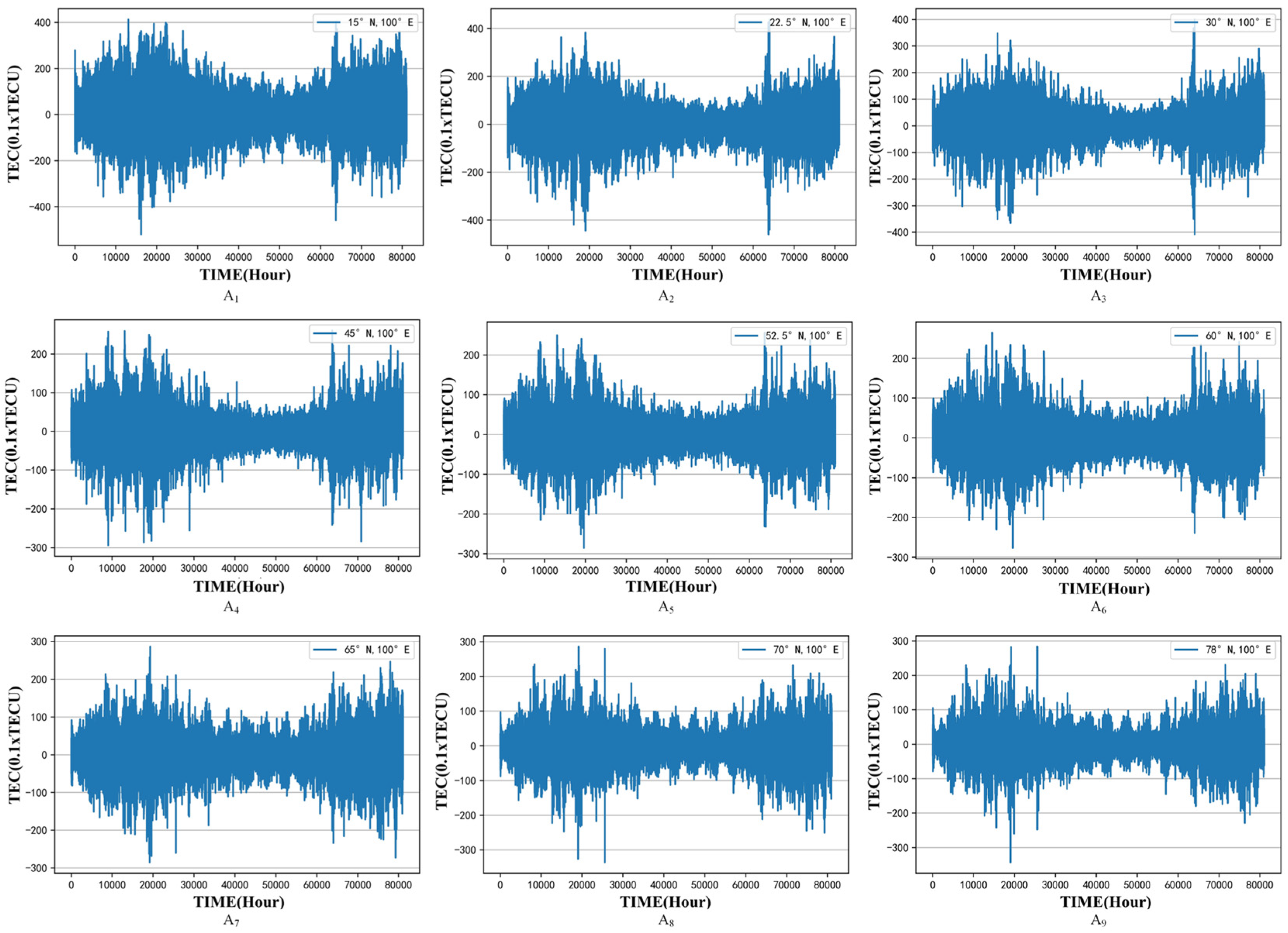
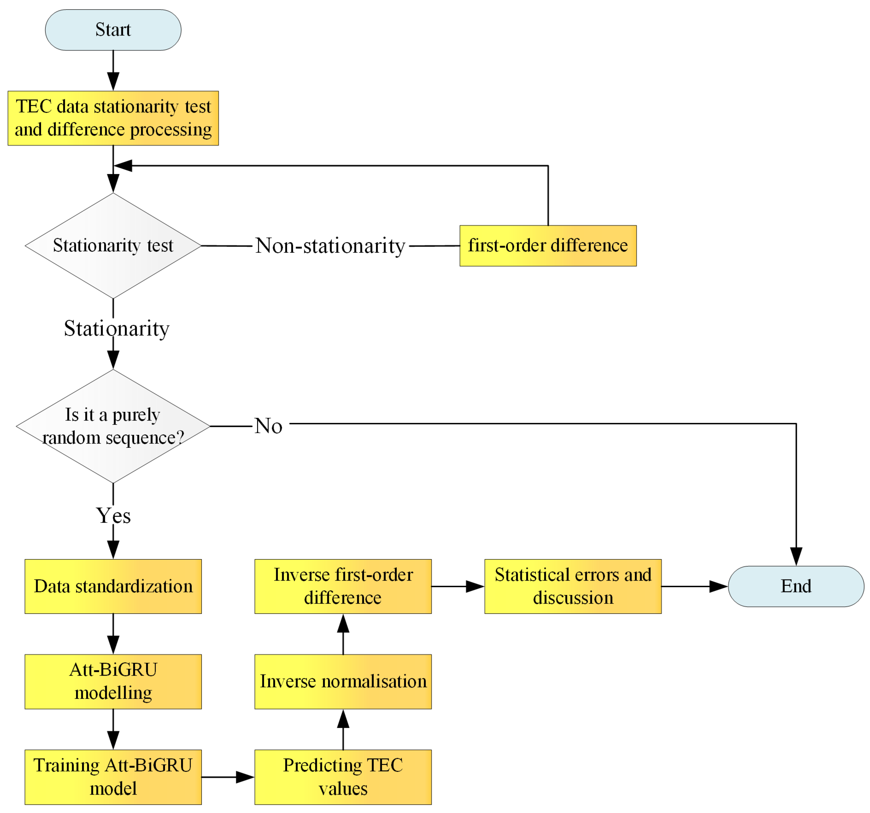
2.2.1. TEC Data Stationary Test and Difference Processing

TEC prediction is a typical time series analysis problem. Time series stationarity is the basic assumption of time series analysis. Therefore, before TEC prediction, we must first test its stability. This paper uses an ADF test method to test the stationarity of time series. The results show that the original TEC data are non-stationary. It can also be seen from Figure 1 that the average values of TEC values in the 9 regions selected in this paper changes with time, which are obviously non-stationary data; thus, it is impossible to directly use the time series analysis model to predict them. In this paper, the ADF test is used to test the stationarity of time series.
The solution is to carry out the first-order difference processing on the TEC data of the nine regions in turn and turn them into stationary sequences. The calculation formula of the first-order difference is as follows:
Δ x t = x t x t 1
where Δ is the first-order difference operator, and x t is the observation data at time t.
Figure 2 shows the first-order difference effect of TEC data in 9 regions in Figure 1. At this time, the ADF test result shows that the TEC time series after first-order differences are stationary time series.

2.2.2. Pure Randomness Test

Not all stationary time series are predictable. Pure random stationary time series are unpredictable. Therefore, it is necessary to test the pure randomness of the time series after stabilization. In this paper, the LB Test is used to test the pure randomness of the time series. The results of the LB test show that the TEC data after first-order difference processing are not pure random data and can be predicted.

2.2.3. Data Standardization

After difference processing, the original TEC data become a stationary time series. However, the data still change greatly in the entire data space, which will affect the results of data prediction. It is necessary to standardize the data firstly. Therefore, we use min-max scaler method to normalize the first-order difference of TEC between 0 and 1.

2.2.4. Samples Making

The TEC data of nine regions in this paper are selected from 0:00 on 29 March 1998 to 24:00 on 25 April 2015. The total number of observation points in each region is 81,081. After the first-order difference processing, it becomes 81,080. Using the segmentation method with a sliding window of 12, the standardized data are made into samples. Every 12 points are the input of a sample, and the 13th point is the output of this sample. The sliding window is made in turn, with a total of 81,068 samples, 90% of which were used as training samples and the rest as test samples.
The sample making process is shown in Figure 3.
After the samples are made, use the training samples to train our proposed model, and then use the test samples to make predictions. Then, the prediction results are processed by inverse standardization and inverse first-order difference.
The entire experimental process is shown in Figure 4.

2.3. Evaluation Indexes

This paper evaluates the model from two aspects: loss indexes and accuracy index.
Loss indexes are used to evaluate the prediction error. In this paper, three loss indexes are used to evaluate the loss of the model: Mean Square Error (MSE), Mean Absolute Error (MAE), and Mean Relative Error (MRE). Loss indexes mentioned above are computed by the following equations:
MSE = 1 n i = 1 n ( y t r u e y p r e ) 2
MAE = 1 n i = 1 n | ( y t r u e y p r e ) |
MRE = 1 n i = 1 n | ( y t r u e y p r e ) y t r u e |
where n is the number of test samples, y t r u e is the real value of test samples, and y p r e includes the predicted values of test samples. The smaller the loss, the better the performance of the model.
The calculation formula of prediction accuracy selected in this paper is shown as follows.
accuracy = ( 1 1 n i = 1 n | ( y t r u e y p r e ) y t r u e | ) × 100 %
The higher the accuracy, the better the performance of the model.

2.4. Our Proposed Model

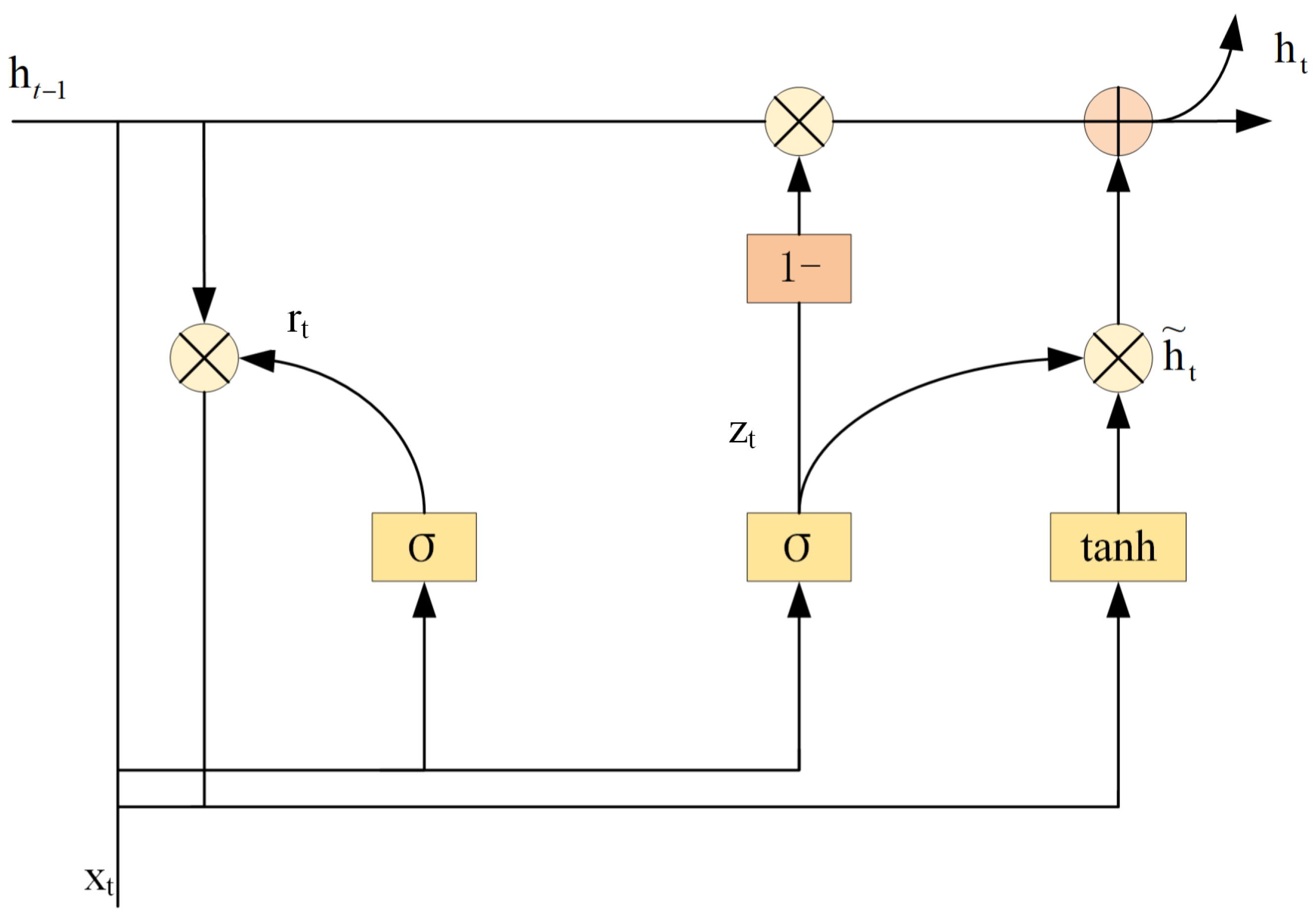
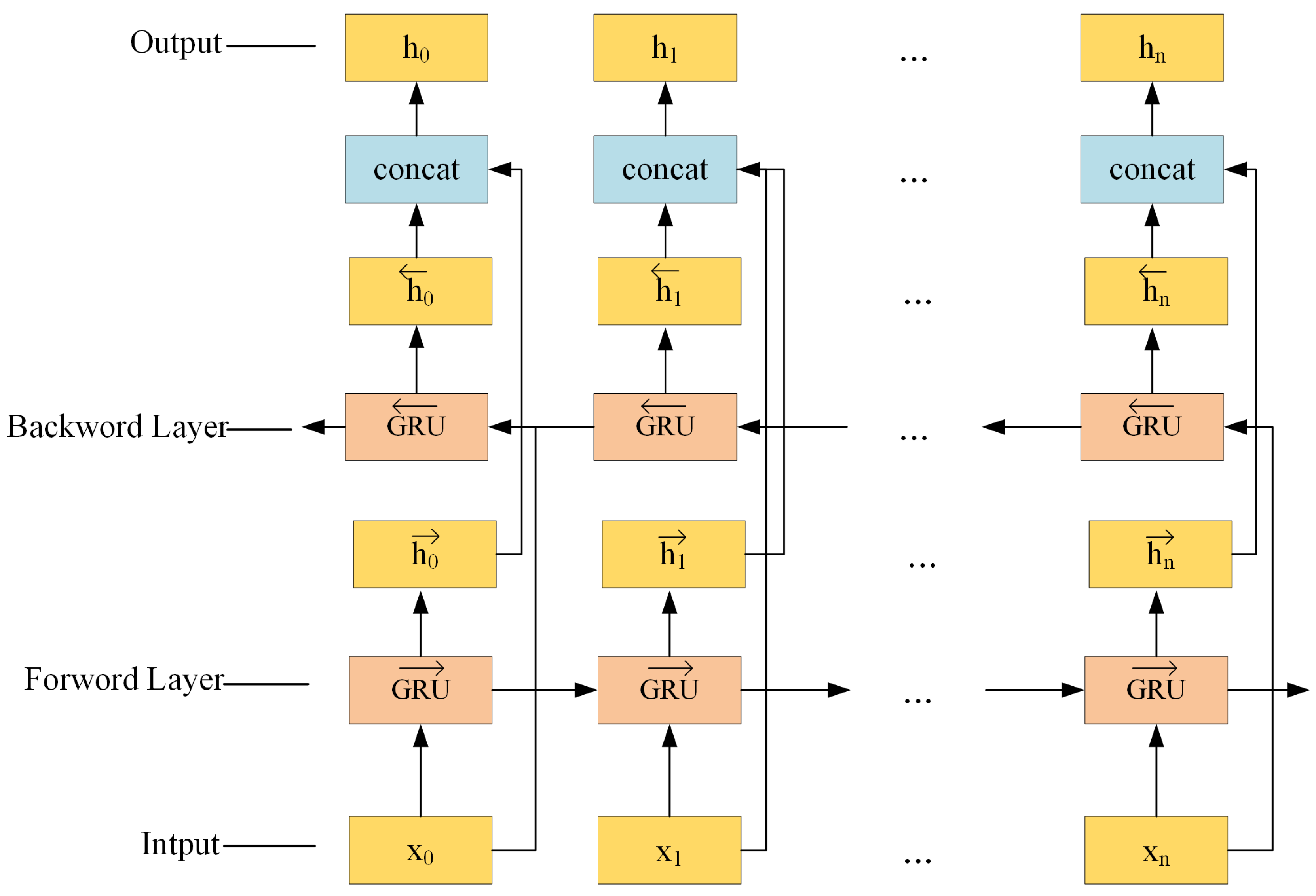
2.4.1. The BiGRU Model

Gate Recurrent Unit (GRU) model is a simplified version of Long Short-Term Memory (LSTM) model that uses two gate structures to effectively alleviate the problem of gradient disappearances. Figure 5 shows the structural overview of a GRU unit. There are only two gates in a GRU unit: an update gate r t and a reset gate z t . Update gate r t controls how much information from the previous hidden state will carry over to the current hidden state. The equations of GRU are described as follows:
r t = σ ( W r × [ x t , h t 1 ] + B r )
z t = σ ( W z × [ x t , h t 1 ] + B z )
h ˜ t = tanh ( W × [ r t h t 1 , x t ] + B h )
h t = ( 1 z t ) h t 1 + z t h ˜ t
where W r , W z , and W represent the weight matrices, represents the element-wise multiplication, [ ] means that the two vectors are connected to each other, x t is the current input, h t 1 is the previous transmitted state, h t is the current transmitted state, σ represents Sigmoid activation function, and B r ,   B z ,   B h are the bias vectors.
The bidirectional gated recurrent unit (BiGRU) model was first proposed by Grüßer-Sinopoli and Thalemann [23]. The base unit of BiGRU model contains a forward-propagated GRU unit and a backward-propagated GRU unit. Therefore, the output layer contains both past information and future information. A structural overview of the bidirectional GRU network is shown in Figure 6.
h t = G R U ( x t , h t 1 )
h t = w t h t + v t h t + b t
Here, G R U ( x t , h t 1 ) presents a forward-propagated GRU unit at time t, and G R U ( x t , h t 1 ) presents a backward-propagated GRU unit at time t. h t is the forward transmitted state, and h t is the reverse transmitted state. w t and v t represent their weights. b t represents bias at time t.

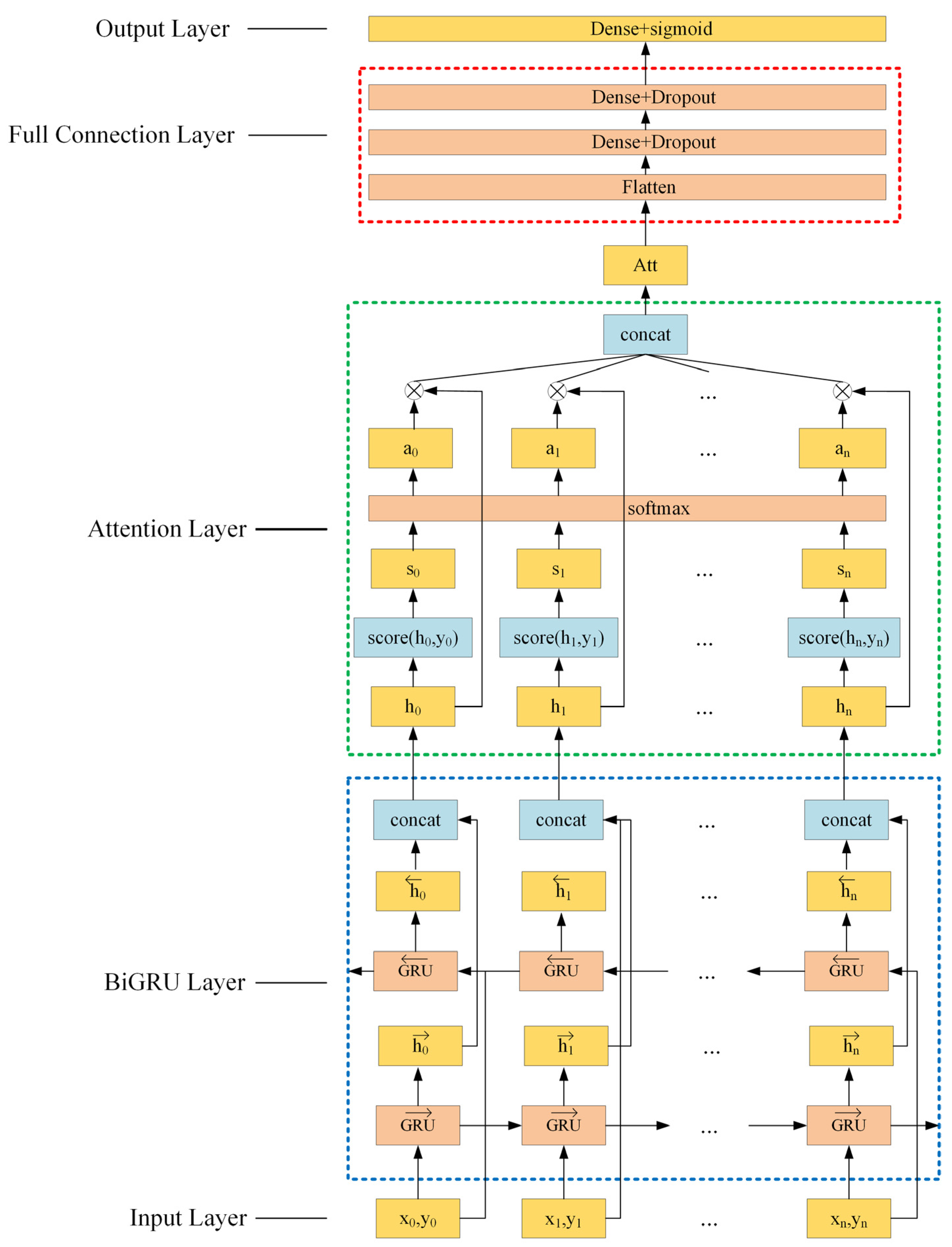
2.4.2. The Proposed Attentional BiGRU Model for TEC Prediction

Our proposed model is a Sequence-to-Sequence model, which means that we predict the output sequences using the input sequences. In our study, TEC data are organized as sequences of input and output pairs. Figure 7 illustrates the architecture of proposed Attentional BiGRU model. The network configuration setup consists of five layers: the input layer, the BiGRU layer, the attention layer, the full connection layer, and the output layer.
A schematic diagram of the proposed Attentional BiGRU is shown in Figure 7.

3. Results and Discussion

3.1. Optimal Parameters of the Proposed Attentional BiGRU Model

After the model is built, the next step is to train the model. In this paper, we train our model on data-set from regions A1. Using Attentional BiGRU for TEC modeling, there are five important parameters that have a significant impact on prediction performance: two model parameters and three training parameters.
Two model parameters include the number of hidden layer neurons and activation function. The three training parameters include optimizer, batch_size, and learning rate. The influence of these five parameters will be discussed one by one below.

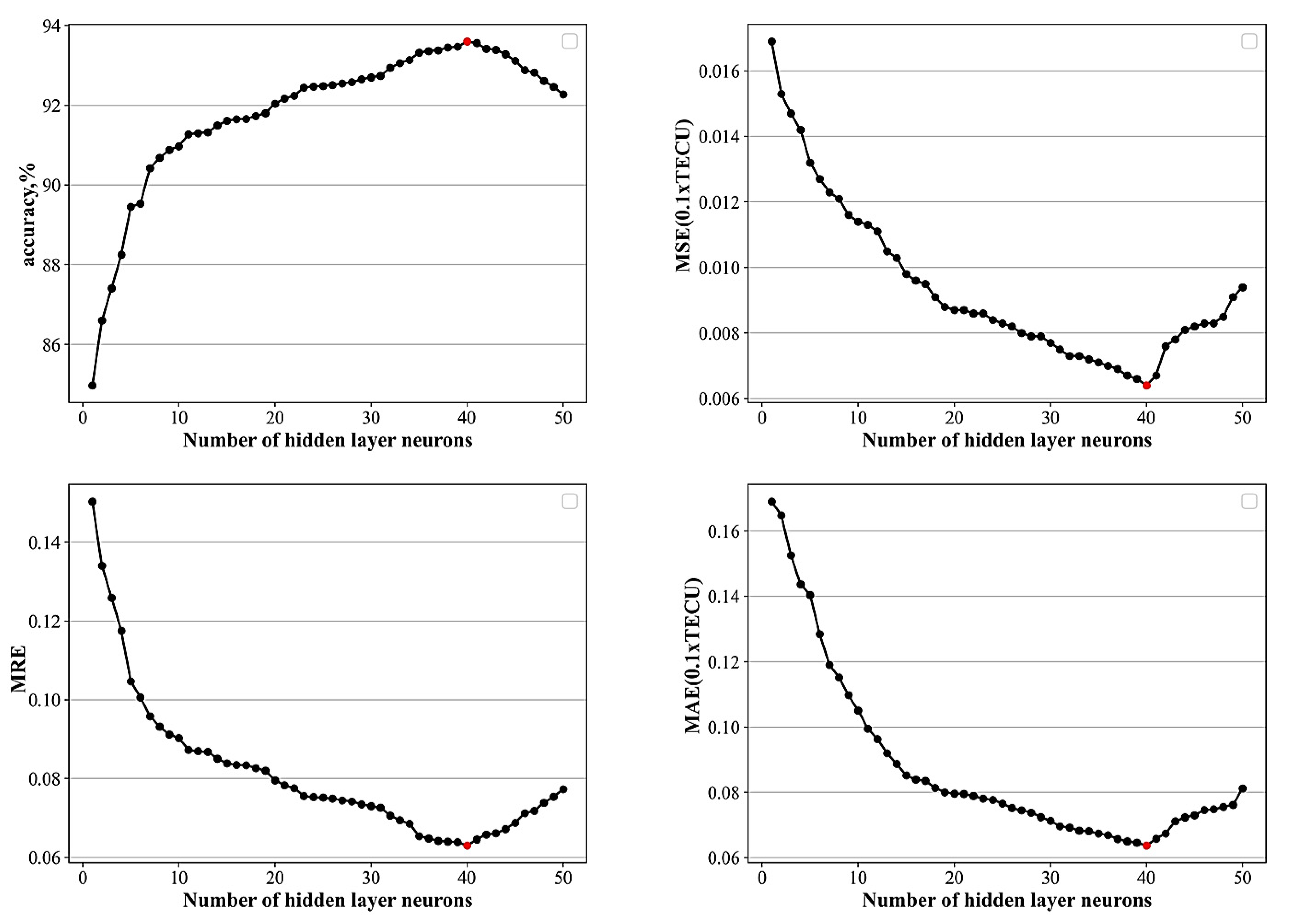
3.1.1. Effect of Model Parameters on Prediction Performance

Number of Hidden Layer Neurons
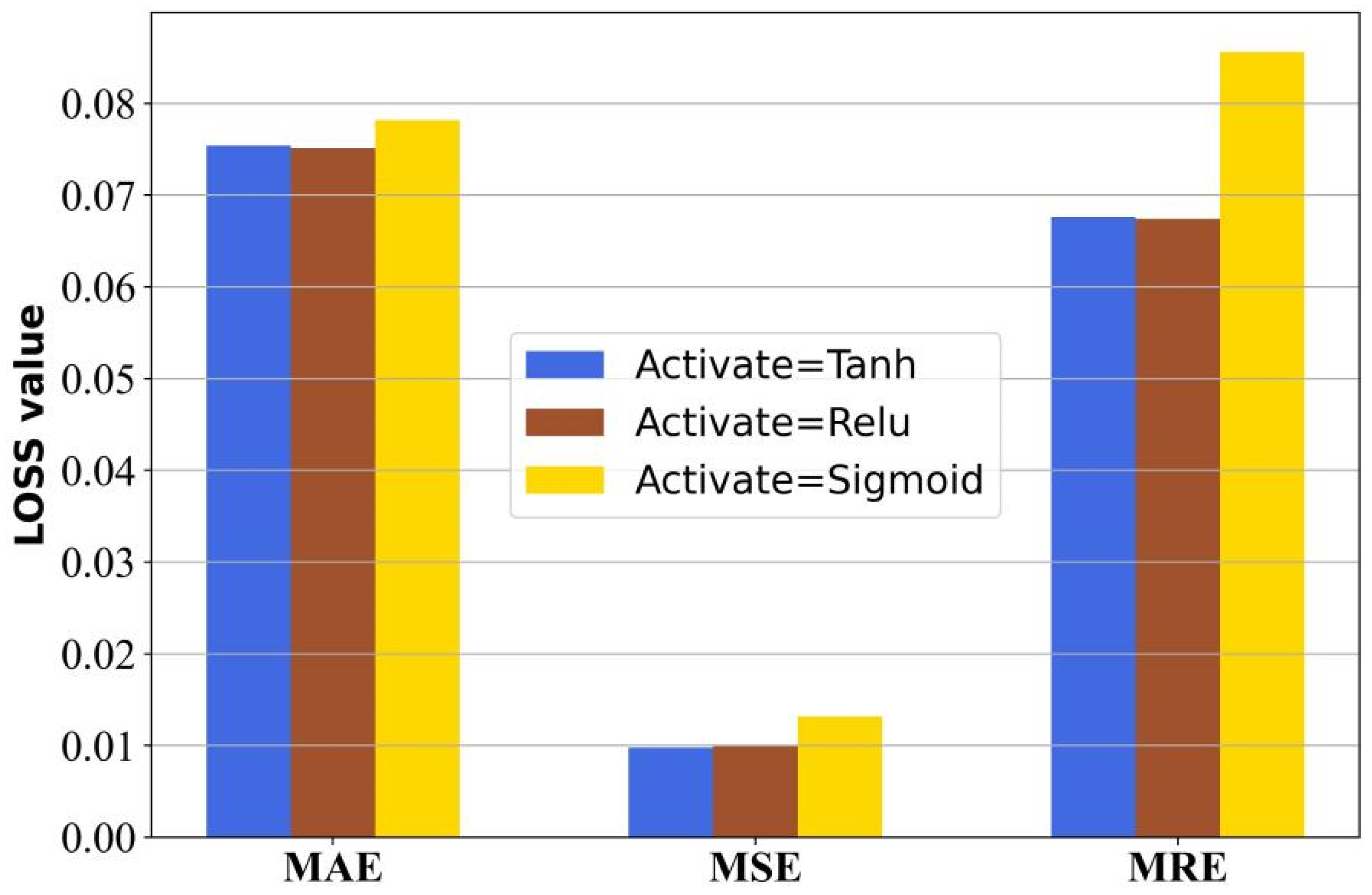
The number of hidden layer neurons (expressed by the parameter units) plays an important role in prediction accuracy. Too many neurons in the hidden layer will lead to over fitting of the model, and too few will lead to under fitting. In this paper, the number of hidden layer neurons ranges from 1 to 50. The effects of different number of neurons on prediction performance are shown in Figure 8.
As observed from Figure 8, the prediction accuracy of the model gradually increases with the increase in the number of hidden layer neurons. When the number of hidden layer neurons is 40, the prediction accuracy of the proposed model reaches the maximum, which is 93.26%. After that, with the increase in the number of hidden layer neurons, the prediction accuracy of the model began to decline, indicating that there was over fitting.
With the increase in the number of hidden layer neurons, MSE, MRE, and MAE decreased gradually. When the number of hidden layer neurons is 40, MSE reaches the minimum value, and when the number of hidden layer neurons is 40, MRE and MAE reach the minimum value.
Therefore, the number of neurons in the hidden layer (units) parameter is set to 40.

Activation Function

The activation function is another important factor affecting the prediction’s results. The activation function is used to introduce non-linearity into the model so that the model can simulate more complex situations. There are three commonly used activation functions: Sigmoid, Tanh, and Relu.
The sigmoid activation function is as follows.
f ( x ) = 1 1 + e x
The tanh activation function is as follows.
f ( x ) = 1 e x 1 + e x
The Relu activation function is as follows:
f ( x ) = { x x > 0 0 x 0
where x represents the total input of the model, and f ( x ) represents the output of the model.
The three activation functions are tested in this paper. The effects of different activation functions on the performance of the model are shown in Figure 9. The specific values are shown in Table 2.
It can be seen from Figure 9 and Table 2 that the performance of the proposed model is the best when the Relu activation function is used.

3.1.2. Effect of Training Parameters on Prediction Performance

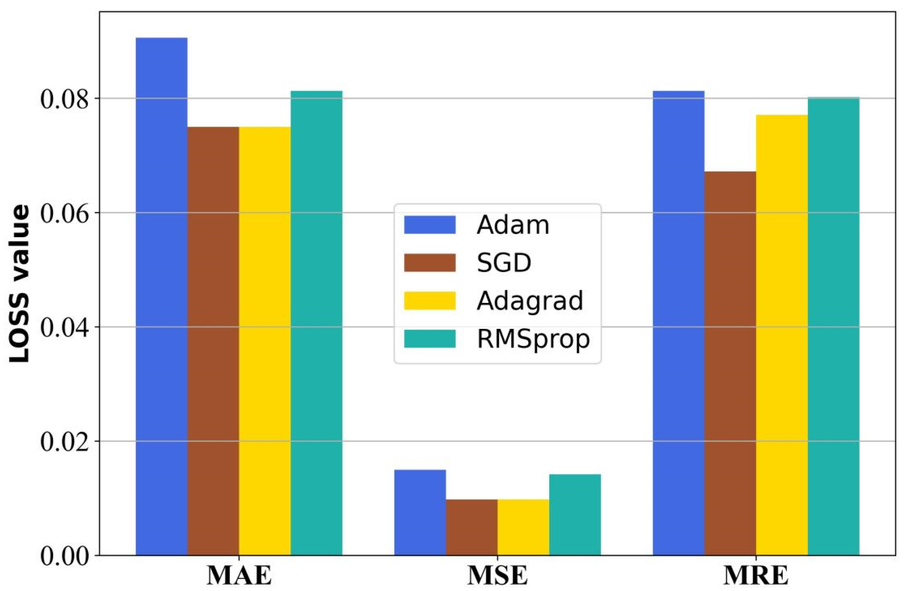
Optimizer Javascript: Void (0)

In the process of model error back propagation, the optimizer guides each parameter of the loss function to update in the correct direction so that the updated value of the loss function continues to approach the global minimum; thus, it plays a vital role in model training. This paper compares four commonly used optimizers: Adam, SGD, Adagrad, and RMSprop. These optimizers are briefly described below:
Adam: Adaptive Moment Estimation (Adam) is an optimizer that computes adaptive learning rates for each parameter and keeps an exponentially decaying average of the past gradients [24].
SGD: Stochastic gradient descent (SGD) is an optimizer that updates parameters for each training input x(i) and its output y(i) [25].
Adagrad: A gradient-based optimizer that adapts the learning rate to the parameters [26].
RMSprop: An optimizer that supports adaptive learning rates [27].
The influence of the four optimizer parameters on the prediction error of the proposed model is shown in Figure 10, and the specific values are shown in Table 3.
As can be seen from Table 3 and Figure 10, when the optimizer is SGD, the prediction performance of the model proposed is the best.

Influence of Batch_Size

In the process of model training, in order to reduce the training time, not all training samples are placed into the model, but a part is randomly selected from the training samples each time, and its quantity is determined by parameter Batch_Size. In order to speed up the training time of gradient descent algorithm, the Batch_Size value is usually an integer power of 2 [28]. When Batch_Size is too large, model training is too slow, and a Batch_Size that is too small size leads to a non-convergence of loss function. In this paper, we experiment with four possible Batch_Size: 16, 32, 64, and 128. The experimental results are shown in Table 4.
As observed from Table 4, when Batch_Size is 32, the performance of the model is the best.

Influence of Learning Rate (LR)

The learning rate (LR) represents the range of each parameter update when the gradient descent method is used to solve find the optimal parameters of the model. If the learning rate is too large, the model cannot easily converge, and if it is too small, the training time of the model will be too long. In this paper, according to experience, five cases of LR = 0.1, LR = 0.05, LR = 0.01, LR = 0.005, and LR = 0.001 are discussed. The experimental results are shown in Table 5.
It can be seen from Table 5 that when LR = 0.1, LR = 0.05, and LR = 0.01, the prediction loss of the model is relatively large. This is because the initial learning rate is large, and the model will fall into the local optimal solution or jump left and right near the optimal solution, resulting in a large training error. When LR = 0.001, the training losses of MSE, MAE, and MRE all reach the minimum. Thus, the best learning rate (LR) is 0.001.

3.2. Comparison with DNN, ANN, RNN, LSTM, GRU, and BiLSTM on Different Latitudes

We select five deep learning time series models, namely DNN, ANN, RNN, LSTM, GRU, and BiLSTM to compare with our proposed Attentional BiGRU. In these comparison models, ANN, RNN, and LSTM have been used in TEC prediction in other studies [12,13,18,19].
All experiments were carried out using the data introduced in Section 2.1 according to the data processing method introduced in Section 2.2. The experimental results are described in Table 6, Table 7 and Table 8.
It can be seen in Table 6, Table 7 and Table 8 that the performance of the proposed Attentional BiGRU model achieved better performances (MAE, MSE, MRE, and accuracy) than the other comparison models.

3.3. Experiments in High and Low Solar Activity Year

The ionosphere is strongly influenced by solar activity. The ionospheric electron density variation is greater in high solar activity years than in low solar activity years [29,30]. To further analyze the performance of the proposed model, research data are divided into low solar activity (LSA) and high solar activity (HSA) periods, and comparative experiments were carried out.
LSA periods: From 0:00 on 1 October 2009 to 24:00 on 31 October 2009, 403 are sample points as the stationary periods test set for prediction since solar activity is not frequent during this period; the Ionospheric TEC is relatively stable.
HSA periods: At each location in Table 1, we select data from 0:00 on 1 October 2003 to 24:00 on 31 October 2003, with 403 sample points as non-stationary periods test set because Ionospheric TEC data were disturbed violently due to the frequent solar activity during this period.
The prediction effect of the proposed model in LSA and HSA is shown in Figure 11 and Figure 12.
Experimental results are shown in Table 9 and Table 10. Comparisons of prediction accuracy between LSA and HSA at different latitudes are shown in Figure 13.
As observed from Figure 13, using the model proposed in this paper to predict the ionospheric TEC, its prediction performance is greatly affected by latitude. The higher the latitude, the higher the prediction accuracy of our proposed model.
It also can be seen that the prediction accuracy of the model is affected differently by solar activity in different latitudes. In the middle latitudes, the prediction accuracy of the model in the LSA periods is similar to that in the HSA periods; that is, in the middle latitudes, the prediction accuracy of the model is hardly affected by solar activity. Around low latitudes and high latitudes, the prediction accuracy of LSA periods is significantly higher than that of the HSA periods. That is to say that in middle latitudes, the prediction accuracy of the model is less affected by solar activity, and in other areas, the model is greatly affected by solar activity.

4. Conclusions

In this study, a BiGRU model with an attention mechanism is proposed in ionospheric TEC prediction. The results indicate that the MSE, MAE, and MRE of the proposed model is smaller than those of DNN, LSTM, BiLSTM, and GRU. The accuracy of the proposed model is greater than that of the four models compared. We studied the effects of different latitudes on the prediction performance of the model. The results show that the higher the latitude, the higher the prediction accuracy of our proposed model. We also studied the effect of solar activity on prediction performance. The experimental results show that, in middle latitudes, the prediction accuracy of the model is less affected by solar activity, and in other areas, the model is greatly affected by solar activity.
For further studies, the author will further study the Ionospheric TEC grid data prediction based on deep learning.

Author Contributions

Writing—original draft and Methodology, D.L.; Writing—review and editing, H.L. (HaiJun Liu); Validation and Resources, H.L. (HuiJun Le); Formal analysis, J.H.; Supervision, J.Y.; Data curation, L.L.; Investigation, Y.W. All authors have read and agreed to the published version of the manuscript.

Funding

This research was funded by the Fundamental Research Funds for the Central Universities (No. ZY20215148), College Students’ innovation and entrepreneurship training program of the Institute of Disaster Prevention and Technology (No. 202111775018X).

Institutional Review Board Statement

Not applicable.

Informed Consent Statement

Not applicable.

Data Availability Statement

Publicly available datasets were analyzed in this study. Ionospheric TEC data can be found here: [https://pan.baidu.com/s/1yoJZd9MKWc_COcbK5Xk_XA, accessed on 28 June 2022].

Acknowledgments

Thank the Center for Orbit Determination of Europe (CODE) for the TEC data. Thanks to Le HuiJun of the Chinese Academy of Sciences for the advice and suggestion.

Conflicts of Interest

The authors declare no conflict of interest.

References

  1. Kaselimi, M.; Voulodimos, A.; Doulamis, N.; Doulamis, A.; Delikaraoglou, D. A causal long short-term memory sequence to sequence model for TEC prediction using GNSS observations. Remote Sens. 2020, 12, 1354. [Google Scholar] [CrossRef]
  2. Tan, S.; Zhou, B.; Guo, S.; Liu, Z. Research on COMPASS navigation signals of China. Chin. Space Sci. Technol. 2011, 31, 9. [Google Scholar]
  3. Sharma, G.; Mohanty, S.; Kannaujiya, S. Ionospheric TEC modelling for earthquakes precursors from GNSS data. Quat. Int. 2017, 462, 65–74. [Google Scholar] [CrossRef]
  4. Meza, A.; Gende, M.; Brunini, C.; Radicella, S.M. Evaluating the accuracy of ionospheric range delay corrections for navigation at low latitude. Adv. Space Res. 2005, 36, 546–551. [Google Scholar] [CrossRef]
  5. Karpov, I.V.; Karpov, M.I.; Borchevkina, O.P.; Yakimova, G.A.; Koren’Kova, N.A. Spatial and temporal variations of the ionosphere during meteorological disturbances in December 2010. Russ. J. Phys. Chem. B 2019, 13, 714–719. [Google Scholar] [CrossRef]
  6. Jiang, H.; Liu, J.; Wang, Z.; An, J.; Ou, J.; Liu, S.; Wang, N. Assessment of spatial and temporal TEC variations derived from ionospheric models over the polar regions. J. Geod. 2019, 93, 455–471. [Google Scholar] [CrossRef]
  7. Li, Z.; Yang, B.; Huang, J.; Yin, H.; Yang, X.; Liu, H.; Zhang, F.; Lu, H. Analysis of Pre-Earthquake Space Electric Field Disturbance Observed by CSES. Atmosphere 2022, 13, 934. [Google Scholar] [CrossRef]
  8. Sivavaraprasad, G.; Deepika, V.S.; Rao, D.S.; Kumar, M.R.; Sridhar, M. Performance evaluation of neural network TEC forecasting models over equatorial low-latitude Indian GNSS station. Geod. Geodyn. 2020, 11, 192–201. [Google Scholar] [CrossRef]
  9. Qiao, J.; Liu, Y.; Fan, Z.; Tang, Q.; Li, X.; Zhang, F.; Song, Y.; He, F.; Zhou, C.; Qing, H.; et al. Ionospheric TEC data assimilation based on Gauss–Markov Kalman filter. Adv. Space Res. 2021, 68, 4189–4204. [Google Scholar] [CrossRef]
  10. Yue, X.A.; Wan, W.X.; Liu, L.B.; Le, H.J.; Chen, Y.D.; Yu, T. Development of a middle and low latitude theoretical ionospheric model and an observation system data assimilation experiment. Chin. Sci. Bull. 2008, 53, 94–101. [Google Scholar] [CrossRef]
  11. Akhoondzadeh, M. A MLP neural network as an investigator of TEC time series to detect seismo-ionospheric anomalies. Adv. Space Res. 2013, 51, 2048–2057. [Google Scholar] [CrossRef]
  12. Yakubu, I.; Ziggah, Y.Y.; Asafo-Agyei, D. Appraisal of ANN and ANFIS for Predicting Vertical Total Electron Content (VTEC) in the Ionosphere for GPS Observations. Ghana Min. J. 2017, 17, 12–16. [Google Scholar] [CrossRef]
  13. Watthanasangmechai, K.; Supnithi, P.; Lerkvaranyu, S.; Tsugawa, T.; Nagatsuma, T.; Maruyama, T. TEC prediction with neural network for equatorial latitude station in Thailand. Earth Planets Space 2012, 64, 473–483. [Google Scholar] [CrossRef] [Green Version]
  14. Inyurt, S.; Sekertekin, A. Modeling and predicting seasonal ionospheric variations in Turkey using artificial neural network (ANN). Astrophys. Space Sci. 2019, 364, 62. [Google Scholar] [CrossRef]
  15. Huang, Z.; Yuan, H. Ionospheric single-station TEC short-term forecast using RBF neural network. Radio Sci. 2014, 49, 283–292. [Google Scholar] [CrossRef]
  16. Habarulema, J.B.; McKinnell, L.A.; Cilliers, P.J. Prediction of global positioning system total electron content using neural networks over South Africa. J. Atmos. Sol. Terr. Phys. 2007, 69, 1842–1850. [Google Scholar] [CrossRef]
  17. Zaremba, W.; Sutskever, I.; Vinyals, O. Recurrent neural network regularization. arXiv 2014, arXiv:1409.2329. [Google Scholar]
  18. Yuan, T.; Chen, Y.; Liu, S.; Gong, J. Prediction model for ionospheric total electron content based on deep learning recurrent neural networkormalsize. Chin. J. Space Sci. 2018, 38, 48–57. [Google Scholar]
  19. Srivani, I.; Prasad, G.S.V.; Ratnam, D.V. A deep learning-based approach to forecast ionospheric delays for GPS signals. IEEE Geosci. Remote Sens. Lett. 2019, 16, 1180–1184. [Google Scholar] [CrossRef]
  20. Ren, Q.; Li, M.; Li, H.; Shen, Y. A novel deep learning prediction model for concrete dam displacements using interpretable mixed attention mechanism. Adv. Eng. Inf. 2021, 50, 101407. [Google Scholar] [CrossRef]
  21. Li, X.; Yuan, A.; Lu, X. Vision-to-language tasks based on attributes and attention mechanism. IEEE Trans. Cybern. 2019, 51, 913–926. [Google Scholar] [CrossRef] [PubMed] [Green Version]
  22. Liu, F.; Zhou, X.; Cao, J.; Wang, Z.; Wang, T.; Wang, H.; Zhang, Y. Anomaly detection in quasi-periodic time series based on automatic data segmentation and attentional LSTM-CNN. IEEE Trans. Knowl. Data Eng. 2020, 34, 2626–2640. [Google Scholar] [CrossRef]
  23. Zhu, Q.; Zhang, F.; Liu, S.; Wu, Y.; Wang, L. A hybrid VMD–BiGRU model for rubber futures time series forecasting. Appl. Soft Comput. 2019, 84, 105739. [Google Scholar] [CrossRef]
  24. Kingma, D.P.; Ba, J. Adam: A method for stochastic optimization. arXiv 2014, arXiv:1412.6980. [Google Scholar]
  25. Ruder, S. An overview of gradient descent optimization algorithms. arXiv 2016, arXiv:1609.04747. [Google Scholar]
  26. Duchi, J.; Hazan, E.; Singer, Y. Adaptive subgradient methods for online learning and stochastic optimization. J. Mach. Learn. Res. 2011, 12, 2121–2159. [Google Scholar]
  27. McMahan, B.; Streeter, M. Delay-tolerant algorithms for asynchronous distributed online learning. Adv. Neural Inf. Process. Syst. 2014, 2, 2915–2923. [Google Scholar]
  28. Wang, Z.; Man, Y.; Hu, Y.; Li, J.; Hong, M.; Cui, P. A deep learning based dynamic COD prediction model for urban sewage. Environ. Sci. Water Res. Technol. 2019, 5, 2210–2218. [Google Scholar] [CrossRef]
  29. Radicella, S.M.; Adeniyi, J.O. Equatorial ionospheric electron density below the F 2 peak. Radio Sci. 1999, 34, 1153–1163. [Google Scholar] [CrossRef]
  30. Rastogi, R.G.; Sharma, R.P. Ionospheric electron content at Ahmedabad (near the crest of equatorial anomaly) by using beacon satellite transmissions during half a solar cycle. Planet. Space Sci. 1971, 19, 1505–1517. [Google Scholar] [CrossRef]
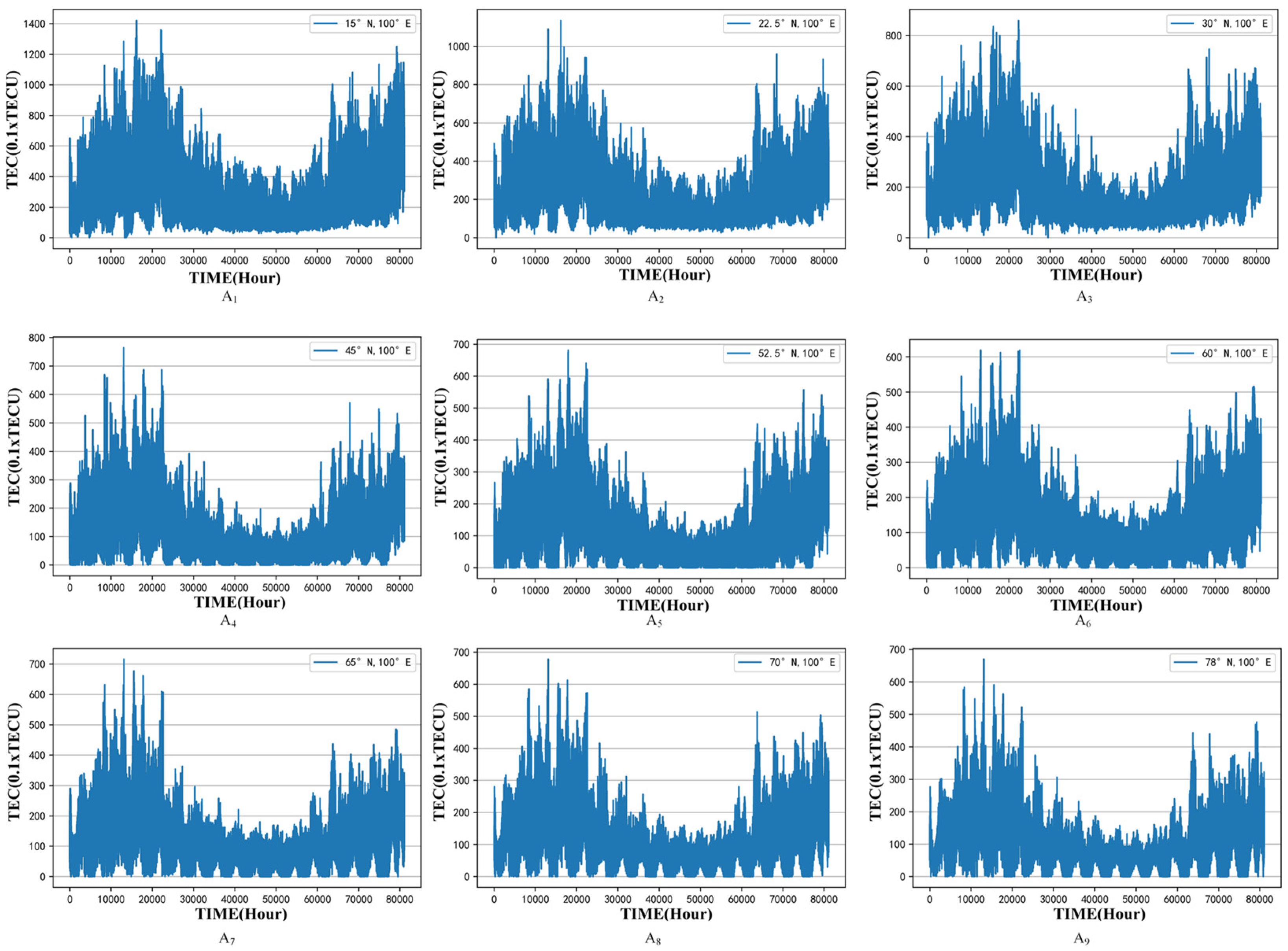
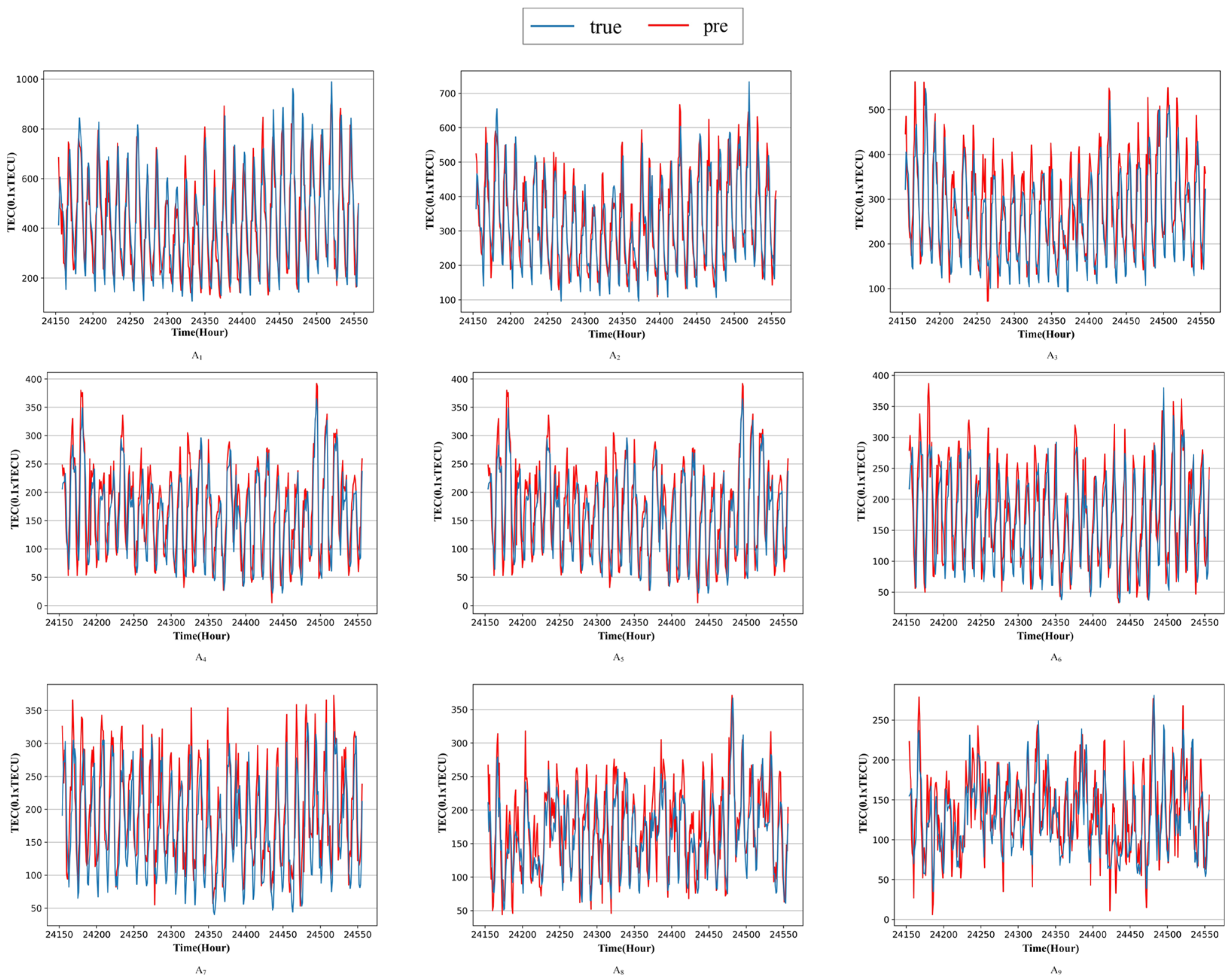
Figure 1. TEC values of nine regions in Table 1 from 1999 to 2014.
Atmosphere 13 01039 g001
Figure 2. The first-order difference of TEC data in 9 regions selected in this paper.
Atmosphere 13 01039 g002
Figure 3. Sample making process in this paper.
Atmosphere 13 01039 g003
Figure 4. Whole experimental process in this paper.
Atmosphere 13 01039 g004
Figure 5. Structural overview of GRU unit.
Atmosphere 13 01039 g005
Figure 6. Structural overview of the bidirectional GRU network.
Atmosphere 13 01039 g006
Figure 7. Schematic diagram of the proposed Attentional BiGRU.
Atmosphere 13 01039 g007
Figure 8. The effects of different number of neurons on prediction performance at A1 (The red dots represent the optimal values of the evaluation indicators).
Atmosphere 13 01039 g008
Figure 9. Effects of different activation functions on the performance of the proposed model at A1. (MSE and MAE are in units of 0.1xTECU).
Atmosphere 13 01039 g009
Figure 10. The effects of optimizer on the prediction loss of the proposed model at A1. (MSE and MAE are in units of 0.1xTECU).
Atmosphere 13 01039 g010
Figure 11. Prediction effect of LSA periods in 9 regions in Figure 1.
Atmosphere 13 01039 g011
Figure 12. Prediction effect of HSA periods in 9 regions in Figure 1.
Atmosphere 13 01039 g012
Figure 13. Comparison of prediction accuracy between LSA periods and HSA periods in different latitudes.
Atmosphere 13 01039 g013
Table 1. Description of all the locations in this paper.
Study Area NumberLongitude and Latitude CoordinatesDescription
A1Bangkok (15° N, 100° E)low latitude regions
A2Lincang (22.5° N, 100° E)
A3Ganzi (30° N, 100° E)
A4Bogdo (45° N, 100° E)middle latitude regions
A5Ojinsky (52.5° N, 100° E)
A6Keremsky (60° N, 100° E)
A7Ewenki (65° N, 100° E)high latitude regions
A8Krasnoyarsk (70° N, 100° E)
A9Arctic ocean (78° N, 100° E)
Table 2. Activation function’s influence at A1.
ActivationMAEMSEMREAccuracy
Tanh0.07540.00980.067693.24%
Relu0.07510.00990.067493.26%
Sigmoid0.07820.01260.085692.44%
Table 3. Effects of optimizer on the prediction loss of the proposed model at A1.
OptimizerMAEMSEMREAccuracy
Adam0.09060.0150.081391.87%
SGD0.07500.00980.067293.28%
Adagrad0.07500.00980.077192.29%
RMSprop0.08130.01420.080291.98%
Table 4. Effects of Batch_Size at A1.
Batch_SizeMAEMSEMREAccuracy
Batch_Size = 160.07500.00980.077292.28%
Batch_Size = 320.07360.00980.065393.47%
Batch_Size = 640.08010.01160.070192.99%
Batch_Size = 1280.08260.01420.076692.34%
Table 5. Influences of learning rates at A1.
LRMSEMAEMREAccuracy
LR = 0.10.01260.08470.107689.24%
LR = 0.050.01050.08200.092690.74%
LR = 0.010.00970.07610.091590.85%
LR = 0.0050.00920.06600.067893.22%
LR = 0.0010.00880.06370.054694.54%
Table 6. Comparison of five methods in three low latitude regions.
AlgorithmIndicatorA1 (15° N, 100° E)A2 (22.5° N, 100° E)A3 (30° N, 100° E)
DNN 0.01350.01130.0270
ANN 0.01320.01300.0127
RNN 0.01420.01230.0103
LSTMMSE0.00750.01540.0082
BiLSTM 0.00820.01190.0065
GRU 0.00980.01260.0088
Att-BiGRU 0.00620.00600.0045
DNN 0.07390.11980.0955
ANN 0.07960.07680.0743
RNN 0.08320.08190.0802
LSTMMAE0.07540.09380.0782
BiLSTM 0.06090.07190.0565
GRU 0.07250.08540.0673
Att-BiGRU 0.05720.06540.0472
DNN 0.09650.09460.0823
ANN 0.08490.08250.0819
RNN 0.08420.08200.0784
LSTMMRE0.06960.06400.0673
BiLSTM 0.06390.06030.0672
GRU 0.06960.06930.0646
Att-BiGRU 0.06340.05980.0597
DNN 90.35%90.54%91.77%
ANN 91.51%91.75%91.81%
RNN 91.58%91.80%92.16%
LSTMaccuracy93.04%93.60%93.27%
BiLSTM 93.61%93.97%93.28%
GRU 93.04%93.07%93.54%
Att-BiGRU 93.66%94.02%94.03%
Table 7. Comparison of five methods in three middle latitude regions.
AlgorithmIndicatorA4 (45° N, 100° E)A5 (52.5° N, 100° E)A6 (60° N, 100° E)
DNN 0.01240.00920.0083
ANN 0.01220.01170.0109
RNN 0.00930.00870.0082
LSTMMSE0.00980.00750.0067
BiLSTM 0.00820.00720.0064
GRU 0.00860.00740.0069
Att-BiGRU 0.00580.00680.0053
DNN 0.09720.09150.0830
ANN 0.07390.07210.0704
RNN 0.07910.07460.0723
LSTMMAE0.07840.06450.0673
BiLSTM 0.06730.06570.0642
GRU 0.07400.06200.0691
Att-BiGRU 0.05700.06180.0533
DNN 0.11550.08860.0901
ANN 0.08030.07820.0774
RNN 0.07640.07380.0715
LSTMMRE0.07880.06610.0652
BiLSTM 0.07250.06230.0647
GRU 0.06330.06210.0620
Att-BiGRU 0.05040.05630.0539
DNN 88.45%91.14%90.99%
ANN 91.93%92.18%92.26%
RNN 92.36%02.62%92.85%
LSTMaccuracy92.12%93.39%93.48%
BiLSTM 92.75%93.77%93.53%
GRU 93.67%93.79%93.80%
Att-BiGRU 94.35%94.37%94.61%
Table 8. Comparison of five methods in three high latitude regions.
AlgorithmIndicatorA7 (65° N, 100° E)A8 (70° N, 100° E)A9 (78° N, 100° E)
DNN 0.02570.01140.0091
ANN 0.01040.00960.0090
RNN 0.00760.00710.0070
LSTMMSE0.00650.00470.0036
BiLSTM 0.00740.00510.0034
GRU 0.00670.00450.0057
Att-BiGRU 0.00580.00450.0033
DNN 0.08430.09610.0998
ANN 0.06740.06610.0652
RNN 0.07040.06590.0624
LSTMMAE0.05860.05280.0551
BiLSTM 0.05670.05190.0532
GRU 0.05780.06150.0547
Att-BiGRU 0.05350.04940.0408
DNN 0.08380.08610.0828
ANN 0.07290.06990.0672
RNN 0.06840.06490.0630
LSTMMRE0.06100.05280.0543
BiLSTM 0.05870.04910.0502
GRU 0.05630.04680.0495
Att-BiGRU 0.05480.04640.0378
DNN 91.62%91.39%91.72%
ANN 92.71%93.01%93.28%
RNN 93.16%93.51%93.70%
LSTMaccuracy93.90%94.72%94.57%
BiLSTM 94.13%95.09%94.98%
GRU 94.37%95.32%95.05%
Att-BiGRU 94.52%95.36%96.22%
Table 9. Prediction effect of the proposed model in LSA periods.
IndicatorA1
15° N
A2
22.5° N
A3
30° N
A4
45° N
A5
52.5° N
A6
60° N
A7
65° N
A8
b70° N
A9
78° N
MSE0.01740.01130.01140.01030.00970.00890.00720.00650.0041
MAE0.10330.08690.09130.08910.08530.08070.06100.05340.0433
MRE0.09240.08910.08640.08390.08260.07820.06850.05260.0416
accuracy90.76%91.09%91.36%91.61%91.74%92.18%93.15%94.74%95.84%
Table 10. Prediction effect of the proposed model in HSA periods.
IndicatorA1
15° N
A2
22.5° N
A3
30° N
A4
45° N
A5
52.5° N
A6
60° N
A7
65° N
A8
70° N
A9
78° N
MSE0.01950.01260.01180.01160.01090.01040.00890.00770.0052
MAE0.10480.09340.09260.09170.08700.08270.06810.05670.0459
MRE0.09530.09360.09110.08640.08350.08200.07030.05810.0468
accuracy90.47%90.64%90.89%91.36%91.65%91.80%92.97%94.19%95.32%
Publisher’s Note: MDPI stays neutral with regard to jurisdictional claims in published maps and institutional affiliations.

