Article

Mapping Heat Wave Hazard in Urban Areas: A Novel Multi-Criteria Decision Making Approach

by
Javad Shafiei Shiva
1,*,
David G. Chandler
1 and
Kenneth E. Kunkel
2
1
Department of Civil and Environmental Engineering, Syracuse University, Syracuse, NY 13210, USA
2
North Carolina Institute for Climate and Satellites, North Carolina State University, Asheville, NC 28801, USA
*
Author to whom correspondence should be addressed.
Atmosphere 2022, 13(7), 1037; https://doi.org/10.3390/atmos13071037
Submission received: 19 April 2022 / Revised: 24 June 2022 / Accepted: 27 June 2022 / Published: 29 June 2022
(This article belongs to the Special Issue Urban Heat Islands and Global Warming)

Abstract

:
Global population is experiencing more frequent, longer, and more severe heat waves due to global warming and urbanization. Episodic heat waves increase mortality and morbidity rates and demands for water and energy. Urban managers typically assess heat wave risk based on heat wave hazard, population exposure, and vulnerability, with a general assumption of spatial uniformity of heat wave hazard. We present a novel analysis that demonstrates an approach to determine the spatial distribution of a set of heat wave properties and hazard. The analysis is based on the Livneh dataset at a 1/16-degree resolution from 1950 to 2009 in Maricopa County, Arizona, USA. We then focused on neighborhoods with the most frequent, severe, earlier, and extended periods of heat wave occurrences. On average, the first heat wave occurs 40 days earlier in the eastern part of the county; the northeast part of this region experiences 12 days further extreme hot days and 30 days longer heat wave season than other regions of the area. Then, we applied a multi-criteria decision-making (MCDM) tool (TOPSIS) to evaluate the total hazard posed by heat wave components. We found that the northern and central parts of the metropolitan area are subject to the greatest heat wave hazard and that individual heat wave hazard components did not necessarily indicate heat hazard. This approach is intended to support local government planning for heat wave adaptation and mitigation strategies, where cooling centers, heat emergency water distribution networks, and electrical energy delivery can be targeted based on current and projected local heat wave characteristics.

1. Introduction

Heat waves and extremely hot weather conditions impact human health and infrastructure in urban areas [1]. They are the main reason for weather-related human mortality and morbidity and cause serious air pollution by increasing the possibility of wildfires and ground-level ozone formation [2,3]. From 1986 to 2017, heat waves were responsible for more than 4000 deaths in the United States of America [4]; including the 1995 Chicago and the 1999 Midwest heat waves that caused more than 1600 deaths [5,6]. Elsewhere, the death toll from the 2003 European heat wave was 14,800 people in France, more than 3000 people in Italy, and more than 2900 people in Portugal [7,8,9]. Moreover, the 2010 Russian heat wave was much worse than these events due to the unfortunate death of more than 55,000 people [10,11]. Following a long history of catastrophic heat waves in India, more than 2400 people died in the heat wave of 2015 [12]. Coates et al. [13] reported 473 heat-related fatalities in Australia from 2001 to 2018. Generally, the demographic with the highest mortality rate in urban areas is the urban elderly (over the age of 65), especially those with pre-existing conditions, communication barriers, and low socioeconomic status residents [14,15,16].
Heat waves increase electricity usage for air conditioning and other cooling purposes in many climates [17,18]. Colombo et al. [19] found that a 3 °C rise in the average temperature increased electricity usage by 7% in Canada. In Greece, Cartali et al. [20] showed that a 1 °C temperature rise increased energy usage for cooling by 28%. In Israel, a 4 °C rise in average temperature is expected to leverage peak electricity demand by 10% [21]. These studies support more recent findings of a general linear relation between daily maximum temperature in the range of 28 °C to 40 °C and electrical energy consumption [22].
The performance of thermal and nuclear power plants decreases during prolonged hot weather, due to challenges in their cooling systems, particularly during low-flow season or droughts [23,24,25]. Despite increasing extreme temperatures and heat waves, energy infrastructure has often not been upgraded sufficiently to avoid numerous power failures at local to national scales [17]. For example, the USA and Canada suffered power outages in summer 2003 that lasted for several days and impacted more than 50 million people [26]. During this period one extreme heat event increased the mortality rate in New York City (NYC) by 25% [27].
Heat waves are complex natural hazards that differ spatially by extremity, magnitude, and frequency and present negative impact on humans, infrastructure, and the environment [28,29]. Urban morphology significantly affects the destructive effects of these events [30]. For example, the interaction between urban heat island (UHI) and heat waves results in exacerbated and extended heat wave events. A New York City study demonstrated that during heat waves, mid-afternoon UHI enhanced temperature by 1.5–2.0 °C [1]. Similarly, UHI is a cause of elevated nighttime temperature [31], which increases risk of morbidity and mortality for elderly people and others who rely on overnight cooling for relief [15]. Laaidi et al. [32] found that during the 2003 heat wave in France, exposure to high nighttime minimum temperature was significantly correlated with the elderly mortality rate. This will be exacerbated in the future based on studies that predict the increase in heat wave length by up to 25 days per year [33]. Similar results from studies of the 1995 Chicago heat wave showed the harmful impacts of high nighttime temperature [6]. Several types of urban green infrastructure including parks, street trees, green roofs, and green walls can offset solar heating in various ways due to differences in albedo, heat capacity, and latent heat of vaporization. Estimates of green cooling vary spatially and range from 7 °C [34] to 10 °C [35] for parks and 1.5 °C near street trees, with green walls providing limited cooling near the wall surface [36]. Smith and Roebber [37] modeled green roofs in Chicago, IL, and found that green roofs can decrease local temperatures by up to 3 °C. In addition, some cities are using pavement watering as a temporary solution for urban heat reduction emergency plans [33]. This method helps cities with a lack of available green spaces, while it is useful for those with available water resources for watering purposes [33,38,39].
Heat-related mortality or morbidity risk is a function of exposure, vulnerability, and hazard [40]. Exposure is an important element in assessing heat wave risk; if there is no human exposure to the heat wave, there is no perceived risk [41]. Although humans can acclimatize to a local climate setting, there are limits to the tolerable amount of heat exposure [14]. These limits are narrower for children, elderly people, and during illness [42,43]. Other dimensions of vulnerability include socio-economic status, neighborhood population density, heritage, and education [44,45]. A study across seven US cities found that increased risk of mortality during a heat wave was associated with lower income and housing value, higher percentage of elderly residents, Asian and Pacific Islander ethnicity, young children, and residents with only primary education [46]. Studies also suggest the importance of communication skills and language barriers in determining population vulnerability to heat waves [16,47].
Although many components for vulnerability and heat exposure analyses are well documented, recognition of hazard elements is inconsistent across heat wave risk-assessment studies. Heat waves have different combinations of components including, at least, frequency, intensity, duration, and timing [48,49]. Each of these components can pose a different type of heat wave hazard in urban areas. Harlan et al. [50] found that maximum temperature during a heat wave is the most important component related to the mortality rate increase in Arizona desert cities (USA). Similar results support the importance of maximum temperature in increasing contemporary heat wave hazard [51,52,53]. Differently, other studies point to the importance of nighttime minimum temperature in urban areas, particularly on the mortality increase of vulnerable populations [32,54,55]. In another study, the mean land surface temperature during heat waves was found to be correlated with heat wave mortality [56]. Further, a 1-day lag in maximum temperature is better correlated with increased mortality than maximum daily temperature [57]. Heat wave onset time and duration are important heat wave components that define the hazard [58]. Seasonally, earlier heat waves are more dangerous to human health than those within the expected hot season and significantly raise the mortality rate [58,59,60,61].
The complexity of the impacts of compound heat wave components on human health is most evaluated by two approaches; correlation between the individual heat wave hazard components and the consequent impact [62,63,64] and multivariate regression models that correlate the main heat wave components (i.e., intensity, duration, and timing) to the overall impact of the event [50,65,66]. Although these methods highlight the importance of understanding the impact of various heat wave hazard components, they do not provide a synthetic assessment of multiple factors or the spatial distribution of the heat wave properties. Studies of spatial distribution for a single element of heat hazard are common. Buscail et al. [41] defined a heat wave hazard map for the city of Rennes (France) based on a single temperature measurement during a heat wave, acquired by Landsat Enhanced Thematic Mapper (ETM+). In this regard, maximum temperature is a common heat wave hazard indicator [67,68,69]. A recent study in Zhejiang province, China proposed accumulated daily maximum and minimum temperatures above 35 °C and 26 °C, respectively, as the heat hazard elements [70]. Liu et al. [56] used mean land surface temperature to map heat wave hazard in China. Similarly, Wu et al. [47] argue the mean temperature level across 24 h during a heat wave predicts mortality and morbidity rates better than maximum and minimum temperatures; yet, most studies focus on maximum daytime or nighttime temperature as an indicator of heat wave hazard [71,72,73].
The increased negative impact of some complex heat waves has led to a new multiple element heat wave hazard assessment. In South Korea, the annual frequency of heat waves with daily peak temperature above 33 °C and nighttime minimum temperature above 25 °C were used as metrics in hazard mapping [52]. Savić et al. [74] integrated frequency and intensity of heat waves for heat wave hazard mapping in European cities. Similarly, intensity, duration, and timing of heat waves have been declared as important metrics for hazard mapping in urban areas [75]. Zhang et al. [76] used heat wave frequency and duration to study heat wave mitigation strategies in China. However, many other heat wave components are neglected in these studies. For example, study of heat wave hazard based on nighttime temperature during an early onset heat wave is unavailable in the literature to the best of our knowledge. We argue that heat wave hazard mapping and classification in urban areas requires considering many defined and known attributed components of heat waves.
Here, we propose an analysis that integrates multiple components to develop an assessment approach that is both comprehensive and specific. Accordingly, we introduced a new framework for heat wave hazard mapping based on all components of the event and a multi-criteria decision-making (MCDM) approach. We used the technique for order preference by similarity to an ideal solution (TOPSIS) model to show how considering MCDM methods improves our knowledge of hazard distribution and reveals unseen hazards in urban neighborhoods.

2. Method, Data, and Study Site

2.1. Heat Wave Definition and Components

We know of no universal heat wave definition, and many debates exist on the parameters that should be included to define a heat wave [29]. In this study, we defined a heat wave as an event that has at least two consecutive days with minimum and maximum daily temperatures greater than the 90th percentiles of the historical minimum and maximum daily temperatures (thresholds), respectively. This definition has been widely used before in heat wave studies [15,49,77].
In addition to the traditional heat wave components, including frequency, intensity, duration, and timing [48], the presented analysis determines eight heat wave components based on the available climatological data. This approach provides clear definitions for each of the main heat wave components [49,78,79].
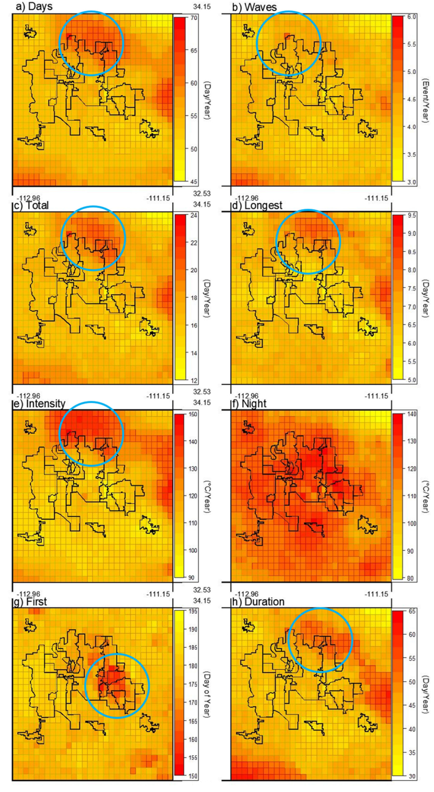
  • Number of hot days (Days): a hot day has both maximum and minimum temperatures higher than defined thresholds.
  • Frequency of heat wave (Waves): number of independent heat waves in each calendar year.
  • Total number of days of heat waves (Total): the cumulative number of days of all heat waves in each calendar year.
  • Longest heat wave event (Longest): the longest heat wave event occurrence in each calendar year.
  • Daytime heat wave intensity (Intensity): the cumulative value of daytime temperatures above the defined maximum temperature threshold during a heat wave.
  • Nighttime heat wave intensity (Night): The cumulative value of nighttime temperatures above the minimum temperature threshold during a heat wave. For example, a heat wave of two consecutive days with the minimum and maximum daily temperatures of 30 °C, 35 °C, 35 °C, and 42 °C at a pixel and the defined thresholds of 28 °C and 33 °C, respectively, has the daytime heat wave intensity and nighttime heat wave intensity of 11 °C and 9 °C, respectively.
  • First heat wave event (First): the day of year for the first day of heat wave in a calendar year.
  • Heat wave season duration (Duration): the period between the first calendar day of heat wave and the last day of the final heat wave in each year.
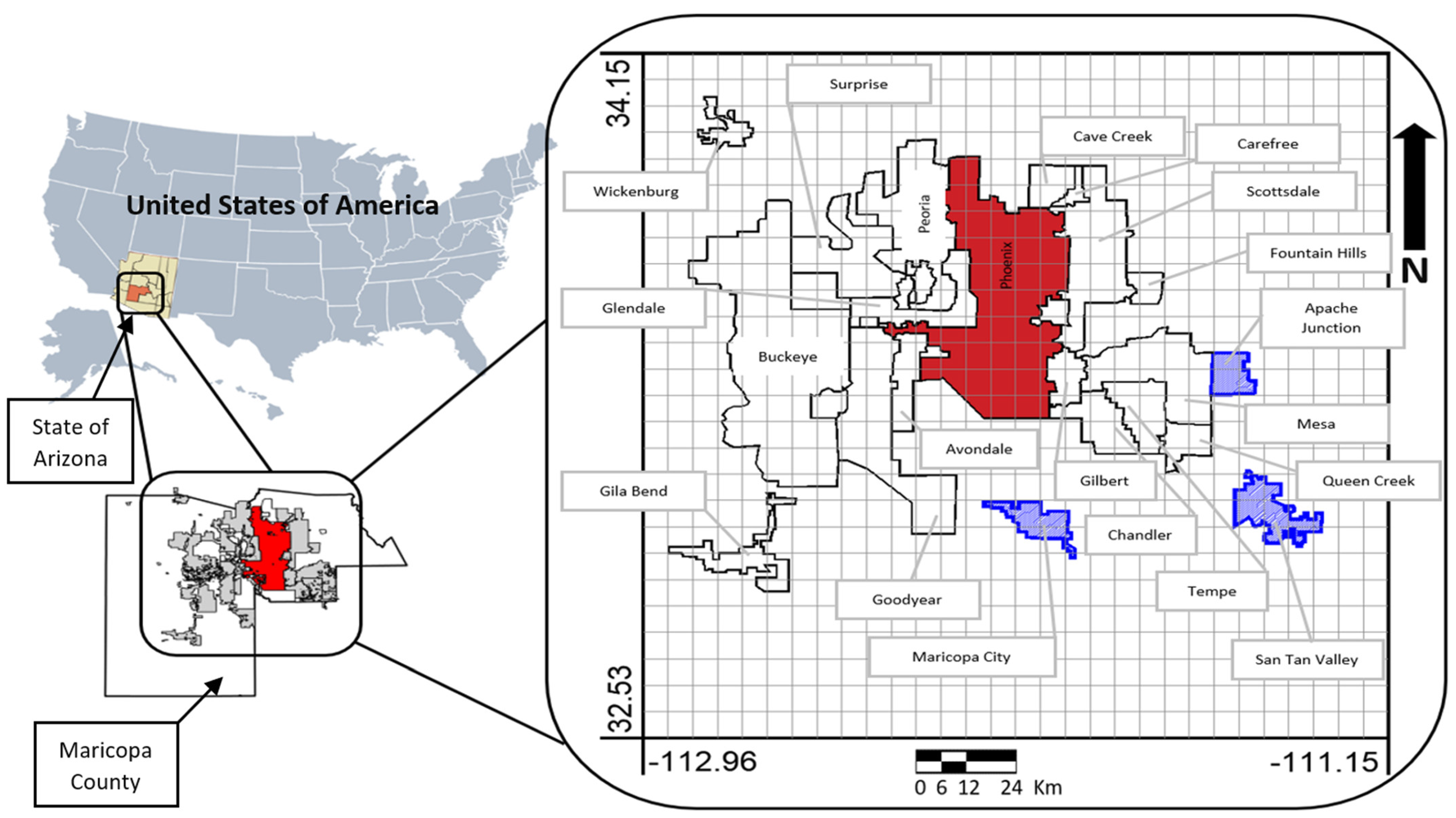
2.2. Study Area

We selected the city of Phoenix, Arizona, USA and the associated metropolitan area (Maricopa County) and three nearby cities from Pinal County (Maricopa City, San Tan Valley, and Apache Junction) for this study (Figure 1). The population of the city of Phoenix and Maricopa County based on 2020 census data were 1,608,139 and 4,420,568, respectively [80]. In addition, based on 2020 census data, the accumulated population of the other three sites was more than 165,000 [80]. Based on the Koppen climate classification, most of this area is located in the hot desert climate category (BWh), where the temperature can exceed 40 °C frequently [81].

2.3. Data Source

We used a daily gridded air temperature product (minimum and maximum temperatures) developed by Livneh et al. [82] based on the interpolation of climate station observations at a 1/16 (~6 km × 6 km) degree resolution. To cover the study area, we obtained the daily maximum and minimum temperatures data from 1950 to 2009 for 810 pixels, 30 longitudinal (−112.9688 to −111.1562), and 27 latitudinal (32.53125 to 34.15625). We examined these data to investigate the average decadal change of minimum and maximum temperatures and then we used a developed code in R to calculate the heat wave properties, defined in Section 2.1 for each of 810 pixels [83].

2.4. Multi-Criteria Decision-Making

Multi-criteria decision-making (MCDM) methods solve complex problems with multiple competing criteria and no optimal solution to satisfy all the decision maker preferences or a procedural goal [84]. For example, most intense heat waves, first heat wave of a season, and longest heat wave are unlikely to coincide in a single neighborhood of a city. Hence, it is not typically possible to find a single region with simultaneous maximum highest heat wave hazard across multiple components simultaneously. Therefore, it is practical to assess each component individually and combine the weighted contributions from all factors in an aggregate assessment [85]. The importance of each component is determined by numerical weight. Some popular multi-criteria decision-making methods include weighted sum model, weighted product model, ELECTRE, TOPSIS, MAUT, PROMETHEE, hybrid fuzzy, VIKOR, and analytical hierarchy process (AHP) [86,87,88]. MCDM methods are popular in spatial studies of various natural hazard and climate extreme events distribution. Aman and Aytac [89] used the AHP method for city scale post-earthquake assembly studies in Turkey. The AHP method is also popular for mapping flood hazard in urban areas based on different flood sources [90,91,92]. Lassandro and Turi [93] used the multi-criteria decision-making approach to evaluate the best response ability of mitigation methods to rising heat waves. For this study, we used the TOPSIS method to investigate how heat wave hazard is spatially distributed across urban areas, based on all the individual heat wave components. This selection was mainly according to the ability of the TOPSIS method to rank the domain pixels based on all defined components of a heat wave, thereby removing any need for independent hazard components [78,84]. In addition, this selection is in line with previous studies on heat waves using TOPSIS multi-criteria decision-making [94,95,96].
Using the TOPSIS method generally includes the following steps [84,97,98]:
  • Calculation of the decision matrix, including alternatives A i (for i = 1 to m, which is the number of pixels, 810 pixels each one ~6 km × 6 km) and criteria C j (for j = 1 to n, which is the number of heat wave hazard components, including Days, Waves, Total, Longest, Intensity, Night, First, and Duration as defined in Section 2.1):
    C 1 C n D = A 1 A m [ x 11 x 1 n x m 1 x m n ]
  • Normalization of the elements in the decision matrix for each criterion:
    N i j = x i j i = 1 i = m x i j 2
  • Calculation of the weighted normalized decision matrix values:
    V i j = W j N i j
    where W j is the weight of each criterion that highlights the importance of that criteria (i.e., each heat wave hazard component as defined in Section 2.1).
  • Finding the best and worst (or ideal and negative ideal) solutions for each criterion:
    A + = { V 1 + ,     , V n +   } = { ( m a x   ( V i j ) | j J ) , ( m i n   ( V i j ) | j J ) }
    A = { V 1 ,     , V n   } = { ( m i n   ( V i j ) | j J ) , ( m a x   ( V i j ) | j J ) }
    where J is associated with benefit criteria and J′ is associated with negative criteria. For example, later heat waves are usually associated with benefit (less harmful) to human health, while higher heat wave intensity is a negative criterion.
  • Calculation of distance from best and worst ideal solutions for each alternative using Euclidean distance method:
    D i + = j = 1 n ( V i j V j + ) 2
    D i = j = 1 n ( V i j V j ) 2
  • Computing the relative closeness to the ideal solution (best or worst case), based on the decision goal:
    C i * = D i ( D i + D i + )
  • Ranking each alternative ( A i ), based on the calculated relative closeness to the ideal solution ( C i * ).
This method ranks neighborhoods (i.e., alternatives or pixels) based on the weighted heat wave component (i.e., criteria). However, to the best of our knowledge, there is no quantitative comparison across all heat wave components. The first heat waves in each calendar year and the most intense heat wave (either higher minimum nighttime temperature or maximum daytime temperature) are the most impactful heat waves. Accordingly, considering greater weights for these factors is inevitable. However, the question remains regarding the quantitative distribution of weights between eight heat wave components, defined in Section 2.1. One practical solution for this problem is to perform a sensitivity analysis for the weights of the inputs to the TOPSIS model to highlight the sensitivity of this analysis to the weights.

2.5. Sensitivity Analysis

Heat wave definition and assigned criteria weights determine the range of possible results of heat wave hazard mapping and classification. To organize the results, we defined six different scenarios to show how the hazard rank of each pixel changes by summation of weighted criteria. In our basic scenario (S1), we assigned the same importance weight to each of the eight heat wave components or MCDM criteria. For Scenario 2 (S2), we assigned the weight of 2 to temperature-related components of the heat wave hazard (i.e., Intensity and Night) and the weight of 1 to the other components. We defined the third scenario (S3) by assigning the weight of 2 to heat wave timing elements (i.e., First and Duration) and 1 to the other components. In the fourth scenario (S4), we assigned the weight of 2 to the number of hot days, frequency of heat waves, total length of heat waves, and longest heat wave event (i.e., Days, Waves, Total, and Longest) and 1 to the other components. Scenario 5 (S5) is defined based on the heat wave components known to have greater human and environmental impacts, including daytime heat wave intensity, nighttime intensity, and first heat wave event (i.e., Intensity, Night, and First) and 1 to the other components. Scenario 6 (S6) is the more extreme representation of the previous scenario (S5), i.e., a weight of 4 to the daytime heat wave intensity, nighttime intensity, and first heat wave event and 1 to the other components. Table 1 summarizes the 6 defined scenarios that we used for sensitivity analysis.

3. Results

First, we present the decadal average changes in minimum and maximum temperatures for the study area from the 1950s to 2000s to show the combined impact of urbanization and climate change on local temperature over six decades. Then, Section 3.2 presents the spatial heat wave components distribution across the study domain. Section 3.3 presents the results of heat wave hazard ranking in 810 pixels by TOPSIS model to show how heat wave hazard is distributed across the region. Eventually, Section 3.4 demonstrates the sensitivity of this study to weights assigned to the decision criteria.

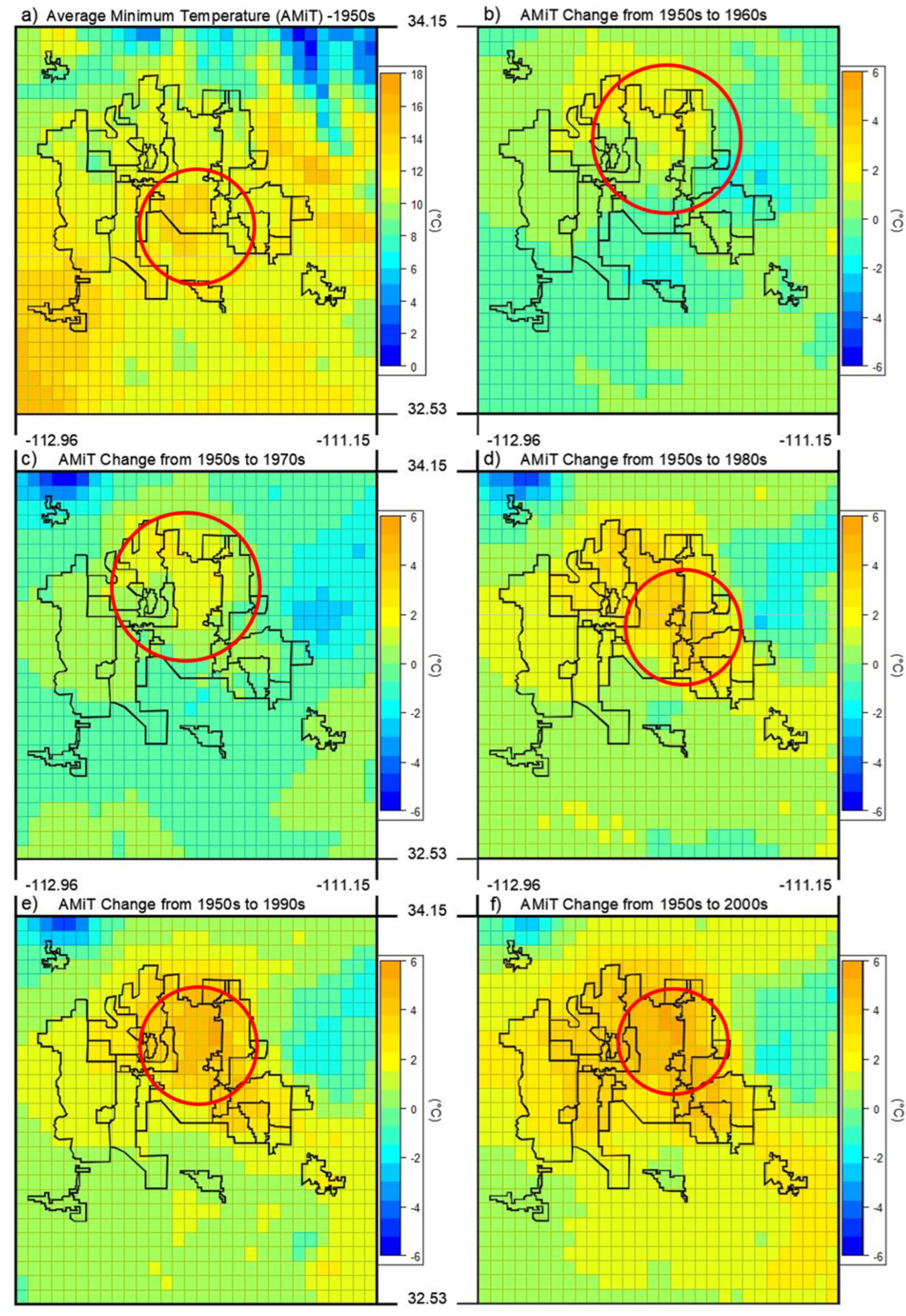
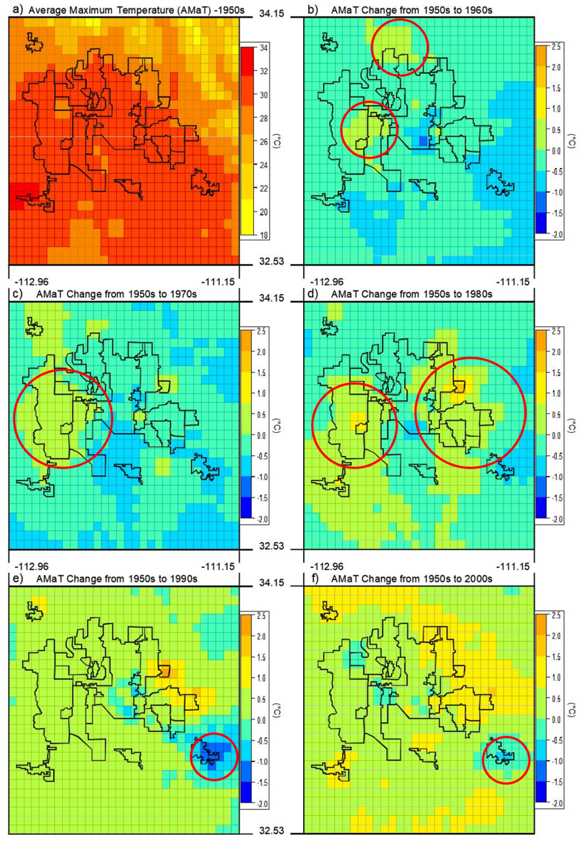
3.1. Temporal Change in Decadal Average Minimum and Maximum Temperatures

We analyzed the decadal average minimum temperature (hereafter AMiT) and decadal average maximum temperature (hereafter AMaT) for the study domain from 1950 to 2009. As shown in Figure 2a, AMiT ranges from 0 °C to 18 °C in the 1950s, with higher temperatures in the southern part of the city of Phoenix (red circle on Figure 2a) and southwest of the study domain and lower temperatures in the northeast part of the domain. Higher AMiT in the 1950s in southern Phoenix can be attributed to the urban heat island effect [99]. During the 1960s and 1970s, AMiT increased in the urbanized areas to the north (red circles on Figure 2b,c), while it decreased in the southern domain of the delineated municipal areas. For the next three decades, AMiT increased steadily, particularly in the urbanized areas. By the 2000s, the decadal average nighttime temperatures for the city of Phoenix had increased by up to 6 °C.
Inspection of AMaT across the study domain shows that the change in average maximum temperature is significantly less than the change in the average minimum temperature. Figure 3a shows the AMaT across the study area in the 1950s, which ranges between 18 °C to 34 °C. Most of the urbanized areas coincided with pixels with the highest value of AMaT (Figure 3a). At this time, north, northeast, and east of the study domain showed the lowest AMaT. In the 1960s there is a general pattern of decrease in AMaT in urban areas, except in parts of the cities of Buckeye and Goodyear (red circle on Figure 3b). This pattern continues in the 1970s, yet the western side of the domain shows an increase in AMaT, while AMaT is decreasing in other regions. In the 1980s, the regions on both sides of the urbanized areas show increasing AMaT compared with the 1950s. Then, in the1990s and 2000s, all urbanized areas have increased AMaT values compared with the 1950s. The only exception in this pattern over five decades is the city of San Tan Valley, which indicated a constant decrease pattern in AMaT until the1990s and then a slight increase in the 2000s (red circles on Figure 3e,f). Interestingly, we found that the maximum change in AMaT is 2.5 °C, which is less than 6 °C change in AMiT for the same study period in the area.

3.2. Heat Wave Components Spatial Distribution

We analyzed the average values of heat wave components (Days, Waves, Total, Longest, Intensity, Night, First, and Duration) for each of the 810 pixels from 1950 to 2009 to understand their spatial properties. We found that the average annual number of Days is between 45 and 70 (Figure 4a), which is greater in the northern parts of the cities of Peoria, Phoenix, Cave Creek, Carefree, and Scottsdale. Days are not always consecutive and the number of heat waves in each year is less than Days at three to six per year. The Waves are distributed nearly evenly across the cities of the study site. However, the total heat wave duration was not equal across the pixels. As shown in Figure 4c, the total days of heat waves, Total, in the study domain is between 12 and 24 days and the northern parts of Peoria, Phoenix, Cave Creek, Carefree, and Scottsdale have more Total than other locations. This pattern was expected following the higher value of Days in those pixels. Other pixels within the cities have a similar total period of heat waves. The longest heat wave events, Longest, range from 5 to 9.5 days within the study domain. As shown in Figure 4d, although there is a slight difference between city pixels, following Days and Total, the longest heat wave events tend to happen in the northern edge of the study cities.
Heat wave intensity during the daytime, Intensity, is between 90 °C and 150 °C. Like Days, Total, and Longest, the higher values of Intensity happen in the northern edge of Peoria, Phoenix, Cave Creek, and Carefree, and most parts of Scottsdale city. Meanwhile, a few areas within the city of Phoenix show higher Intensity compared with their neighborhoods.
The distribution of nighttime heat wave intensity, Night, is completely different from other heat wave properties. Interestingly, the range of Night is like Intensity and equal to 60 °C and varies from near 80 °C to 140 °C. However, the spatial distribution of this component is more disperse than others, showing the importance of considering nighttime effects on temperature separately (Figure 4f). As shown in Figure 4f, San Tan Valley has the lowest value of Night between other cities. Meanwhile, Phoenix has the relatively highest value of Night. The pattern of timing of the first heat wave, First, is closest to the pattern for nighttime in the eastern area and occurs between Julian day 150 and 195 (30 May and 14 July). Accordingly, residents of the area, including southern parts of Scottsdale, Fountain Hills, all of Gilbert city, north and central parts of Mesa, northern parts of Chandler and Tempe, and the center of Phoenix, experience the first heat wave in each year up to one month earlier than the adjacent cities (Figure 4g).
The heat wave season is uneven due to local differences in Duration, which varies between 30 and 65 days, and is typically longer in the northern parts of Peoria, Phoenix, Carefree, Cave Creek, and Scottsdale (Figure 4h). The wide variation of spatial patterns of heat wave components across the study area reveals a pattern of spatially different local maxima, with occasional spatial congruence. For example, higher values of Days, First, and Duration occur in three distinct neighborhoods (Figure 4a,g,h). This finding supports the use of the multi-criteria decision-making tool for heat wave hazard mapping and classification.

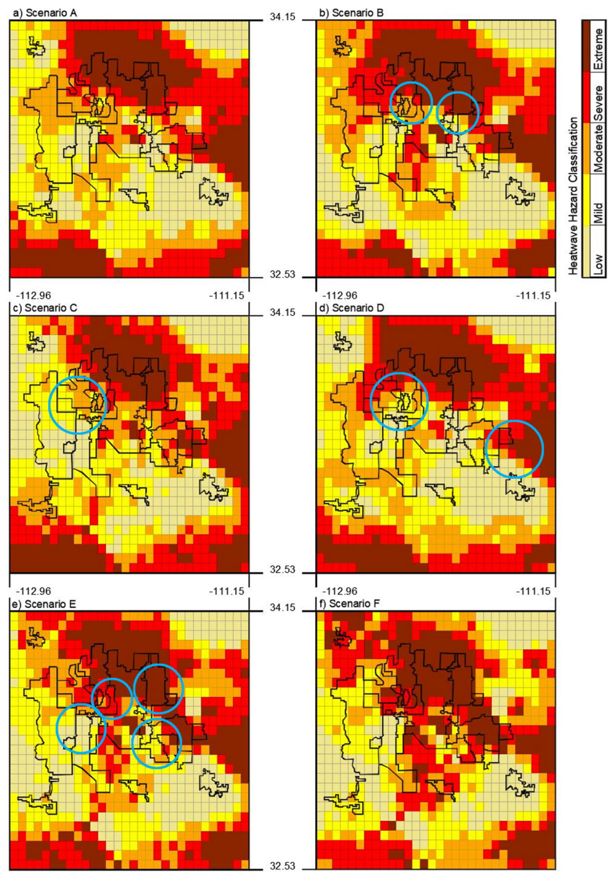
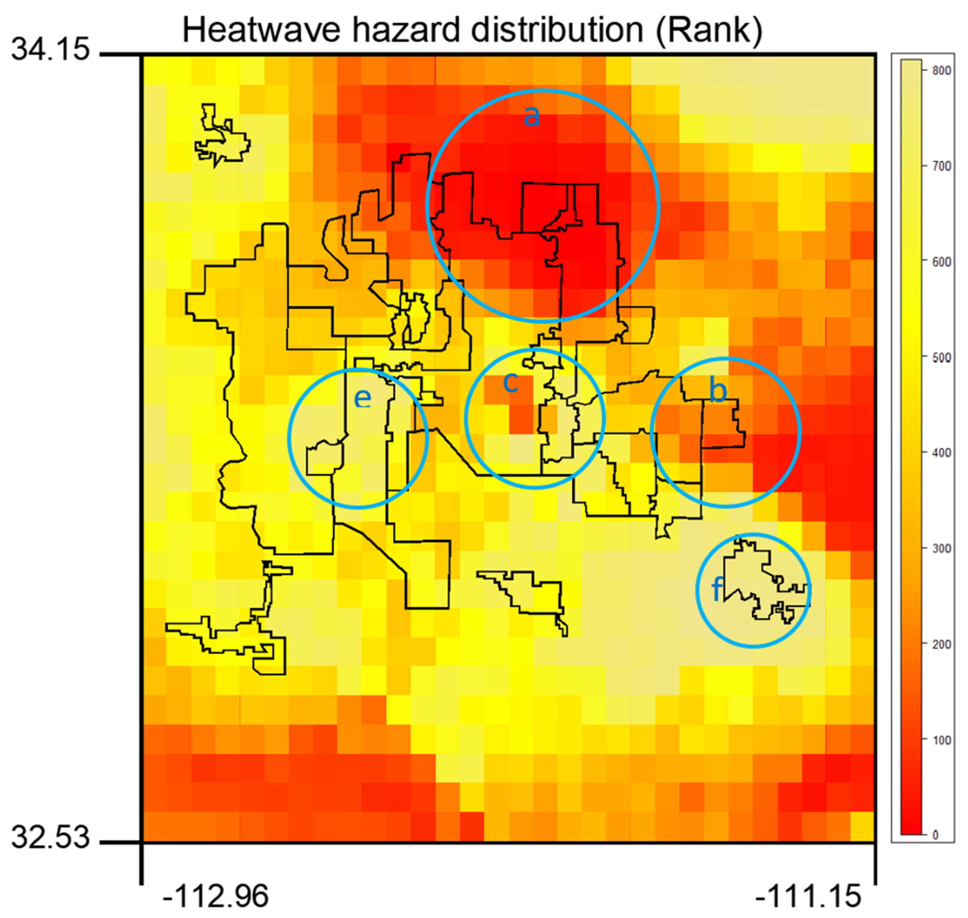
3.3. Heat Wave Hazard Mapping Using TOPSIS

We applied the TOPSIS multi-criteria decision-making model to sort the domain pixels according to the eight defined heat wave components, following the steps described in Section 2.4. The base hazard classification scenario (S1) weighted each heat wave component equally. The pixel rank values indicate the level of heat wave hazard in decreasing rank order (1 to 810) within the map. Figure 5 shows five main regions of greater heat wave hazard, of which only three are in the urbanized area. The first region includes northern Peoria and Phoenix, Cave Creek, Carefree, and most of Scottsdale (Figure 5, Circle a). Similarly, the eastern part of Mesa and all of Apache Junction have higher heat wave hazard (Figure 5, Circle b). This greater hazard follows the spatial distribution of Days, Total, Intensity, First, and Duration shown in Section 3.2 (Figure 4a,c,e,g,h). Surprisingly, we found localized heat wave hazard in southern Phoenix (Figure 5, Circle c). This area did not show high individual heat wave components but scored a greater hazard from multiple contributing hazard elements. Overall, heat wave hazard is extensive north of Surprise and Buckeye, least in Goodyear and Southern Buckeye (Figure 5, Circle e), and San Tan Valley (Figure 5, Circle f).

3.4. Sensitivity Analysis

We defined six scenarios (Table 1) to compare the sensitivity of heat wave hazard classification with the weights of various criteria in this multi-criteria decision-making process. For simplification, we categorized the ranks in five levels of heat wave hazard, including extreme (1 to 162), severe (163 to 324), moderate (325 to 486), mild (487 to 648), and low (649 to 810). This classification is not directly related to the actual hazard posed to human health; rather, the ranks serve to highlight the relative spatial distribution of heat wave hazard. Accordingly, S1 is the base scenario and highlights the classification of heat wave hazard distribution based on equal weights for the criteria (see Section 3.3). We compare other scenarios with S1 to compare the relative change in heat wave hazard categories using different criteria weights. For S2, the combined daytime and nighttime heat wave intensity increases the hazard level in the city of Phoenix from severe to extreme hazard and within the city of Surprise from moderate to severe hazard (Figure 6b). In scenario S3, we found that heat wave hazard decreases in the western part of the study domain, mainly in the city of Buckeye (Figure 6c), and there is no significant change in other locations.
The importance of the weighing of hot days, heat wave frequency, total duration of heat waves, and longest heat wave events for each year are shown by comparison of scenario S1 with S4, S5, and S6. S4 decreases heat wave hazard for the eastern regions, while increasing heat wave hazard from mild to moderate for the cities of Surprise and Buckeye (circles shown on Figure 6d). S5 represents both daytime and nighttime heat wave intensities and heat wave onset time, which have the greatest weight of the eight heat wave components (Table 1). Previous qualitative studies have prioritized these criteria due to the direct effects on human health [59,69,100]. Based on S5, heat wave hazard decreases from moderate to mild for the western part of Buckeye, increases from moderate to severe in southern Surprise, increases from severe to extreme for northern Phoenix, and increases from moderate to severe for the southern part of Phoenix. Following other scenarios, we find no significant change in heat wave hazard classification for cities out of Maricopa County. Similarly, the heavy weighting factor (4) of S6 for heat wave intensity during days and nights and heat wave onset further emphasizes heat wave hazard in urban areas by increasing heat wave hazard level. In this scenario, we observed a change from moderate to mild hazard for the western part of Buckeye, from moderate to severe and extreme in southern Surprise, from severe to extreme for the northern part of Phoenix, and from moderate to severe and extreme for the southern part of Phoenix.

4. Discussion

We found that the average temperature in the greater Phoenix area has increased over the last six decades, extending the results from prior studies [99,101,102], with marked increase in minimum nighttime temperature. We attribute this change to global warming and urbanization and knock-on effects from UHI to the greater nighttime temperature [1]. However, disaggregation and quantification of the individual contributions of climate change and urbanization to increasing temperatures is not within the scope of this research. We observed clear and quantifiable spatial variations in heat wave components across the study area. To the best of our knowledge, this is the first research study that shows the spatial and temporal changes in various heat wave components simultaneously. This finding calls into question the fidelity of current heat wave risk mapping and classification methods. In addition, it echoes a need for more regional and finer scale extreme events studies, particularly for heat waves [47,103].
Traditional heat wave risk studies assume an even distribution of heat hazard [14,104]. This remains the case for studies that recognize different hazard components for risk assessment but rely on temperature as the single indicator of heat wave hazard distribution [41,75]. The result of this study contradicts the previous traditional assumptions by showing how these heat wave hazards change spatially and temporally. Here we demonstrated that heat wave hazard should be independently mapped, along with the exposure and vulnerability components throughout the study area, to achieve more accurate heat wave risk assessments. We propose that this more sophisticated approach can improve the value of high spatial resolution temperature information and, as a result, better heat adaptation and mitigation strategies.
We found that the northern regions of urbanized areas in the study experience more extreme heat days than other areas, while heat wave frequency spatial distribution is nearly even across the study areas. Total length of heat waves follows the pattern of hot days, which was predictable, as the hotter days will result in a higher total length of heat waves. The longest heat wave events occur slightly more frequently in the northern part of the domain. This is likely due to conversion of cropland and loss of cooling by latent heat of evaporation from agricultural fields. A similar research study showed that the shrinkage of green areas in the urban surroundings of Karachi, Pakistan resulted in the excessive nighttime warming and more frequent and extended heatwaves [39]. In agreement with other UHI studies, we found that urbanization is increasing heat wave intensities in urban areas due to UHI [105] and increases heat wave exposure likelihood for residents primarily by increased urban temperatures [15]. Heat wave onset, seasonal duration, and spatial distribution were not predictable. Regions with higher nighttime temperatures experience earlier heat wave seasons. This implies that urbanization amplifies and extends heat wave season timing. In addition, the findings of this study help urban planners to develop mitigation plans more efficiently. It also repeats the importance of green space as an effective mitigation strategy in urban areas. We found that the incidence of heat waves was advanced by as much as 40 days over the study period in some regions; this means earlier extra pressure on water resources and electricity distribution grids.
Despite the measurable values of heat wave components, we can find no study that has developed spatial urban heat wave hazard maps and classification based on heat wave compound properties. Accordingly, we applied a rank-based multi-criteria decision-making tool to integrate a broad set of components to develop hazard maps. Although the presented approach does not determine heat wave hazard for individual pixels, it facilitates broad interpretation of quantitative metrics for adaptation and mitigation plans by presenting relative hazard in the study domain.
Finding a higher hazard rank for the northern and eastern parts of the urban areas was expected. When many individual heat wave components have higher (or highest) values within these regions, it is expected that the MCDM approach points to them as well. Surprisingly, we found the areas in the central part of Phoenix with greater hazard value. Such important findings at this level could be used to guide resources to this heavily populated neighborhood to limit exposure, vulnerability, and heat wave hazard of the residents, where there is very high heat wave risk.
A novel finding of this research was the identification of heat wave hazard regions that are the product of multiple heat wave hazard components. In Phoenix, with the highest population of the study region, we found two primary regions with extremely high heat wave hazard, i.e., the northern and the central parts (Figure 5). Since northern Phoenix is less urbanized than central Phoenix, we propose that central Phoenix has the greatest heat wave hazard. According to the USA National Weather Service (NWS), most heat wave fatalities occur within the resident household [4]. Similar findings confirm that exposure to greater frequency of heat wave hazard increases health risk, especially for vulnerable groups [32,41]. Importantly, this study identified high heat wave hazard where Chuang and Gober [106] found the highest vulnerability and hospitalization rate in Phoenix, supporting the utility of this analysis.
In this study, we found that the lowest heat wave hazard generally occurs in regions with greater green space. The latent heat decreases the temperature within the region and subsequently decreases heat wave occurrences and hazard. This observation encourages the importance of green spaces within urban areas as a natural tool for heat wave mitigation [39,99].

5. Conclusions

We analyzed the decadal average minimum and maximum temperatures changes and heat wave components’ spatial distribution across the 810 pixels (1/16° at 1/16°), covering the Phoenix metropolitan area in Maricopa County located in the state of Arizona, USA from 1950 to 2009. During this period, we demonstrated the potential combined impact of urban heat island and global warming in urban heat stress. If current trends in population growth and urbanization continue to leverage global warming in the Phoenix metropolitan area, more extremely hot days and nights are expected to occur. This study demonstrates that heat wave components are not evenly distributed in the study domain. This analysis is leveraged by a multi-criteria decision-making tool to highlight local areas with enhanced heat wave hazard. To the best of our knowledge, this is the first research study that focuses on the spatial distribution of heat wave components using an MCDM approach. We found that the urban core of Phoenix is among the highest heat wave hazard areas, and agricultural fields and cultivated croplands have the lowest heat wave hazard. This supports the use of green space in mitigation of heat wave hazard. Finally, we performed sensitivity analyses and showed that the heat wave hazard map is insensitive to a change in the selected hazard criteria weights for this city. The products of this study clarify the many differences in quantitative heat wave elements’ variation on a local scale and serve as an example of analysis to support heat wave adaptation and mitigation strategy plans for local government. We argue this new method significantly improves our understanding of heat wave hazard distribution in the urban areas. Consequently, more accurate mitigation plans can be developed for each individual urban setting. Remedial measures in target areas may include schedules for cooling centers, heat emergency water distribution networks, and electrical energy delivery based on regional heat wave characteristics.

6. Research Limitations and Future Directions

This study introduces a new approach to heat wave hazard mapping in urban areas based on the MCDM approach. However, it has a few limitations. In this research, only one heat wave definition has been used. This definition is based on ambient temperature and ignores the impact of humidity and, consequently, apparent temperature or heat index in heat wave definition. Although this definition is commonly used in the field, arguments exist on the benefits of using the heat index. The size of pixels (or smallest areas with assigned data) is 6 km × 6 km. This dimension is reasonable for larger urban studies. However, in dense urban areas, a finer resolution is required for decision-making purposes. Another limitation of this research is the availability of the Livneh data set. The required data for this research were available only for 1950 to 2013 [82], and we used those from 1950 to 2009 to cover the historical changes in heat wave characteristics for 6 decades. In addition, we only used TOPSIS for MCDM analysis. This leaves the impact of MCDM selection in the hazard mapping results unknown. Lack of similar studies in the past regarding this topic for result comparison purposes is another limitation of this research. Although we compared the findings of this study with some previous research, it was impossible to find similar studies that used the MCDM-based approach using different heat wave components in the study area of this work. Accordingly, we propose a direction for future studies and present alternatives and further research as follows:
  • Applying different heat wave definitions, including those based on heat index, to understand the impact of various heat wave measures on the hazard mapping.
  • Using finer resolution, at least for dense urban areas, to understand the impact of different urban structure on heat wave hazard distribution.
  • Analyzing different mortality and morbidity data from the area to understand the correlation between heat hazard and public health. This will help to validate the results of this research in the context of a lack of other similar publications.
  • Using another data set(s) to cover more recent years (i.e., 1950 to 2019 instead of 1950 to 2009.

Author Contributions

Conceptualization, J.S.S., D.G.C. and K.E.K.; methodology, J.S.S.; software, J.S.S.; validation, J.S.S., D.G.C. and K.E.K.; formal analysis, J.S.S.; investigation, J.S.S. and D.G.C.; resources, J.S.S., D.G.C. and K.E.K.; data curation, J.S.S.; writing—original draft preparation, J.S.S.; writing—review and editing, J.S.S., D.G.C. and K.E.K.; visualization, J.S.S.; supervision, D.G.C.; project administration, D.G.C.; funding acquisition, D.G.C. All authors have read and agreed to the published version of the manuscript.

Funding

Financial support for this work was provided via the Urban Resilience to Extremes Sustainability Research Network under National Science Foundation grant AGS-1444755. The APC was funded by the authors.

Institutional Review Board Statement

Not applicable.

Informed Consent Statement

Not applicable.

Data Availability Statement

R code developed for heat wave components analysis and all related data are available in an online and open access data repository [83].

Conflicts of Interest

The authors declare no conflict of interest.

References

  1. Ramamurthy, P.; Li, D.; Bou-Zeid, E. High-Resolution Simulation of Heatwave Events in New York City. Theor. Appl. Climatol. 2017, 128, 89–102. [Google Scholar] [CrossRef]
  2. Song, X.; Wang, S.; Hu, Y.; Yue, M.; Zhang, T.; Liu, Y.; Tian, J.; Shang, K. Impact of Ambient Temperature on Morbidity and Mortality: An Overview of Reviews. Sci. Total Environ. 2017, 586, 241–254. [Google Scholar] [CrossRef]
  3. Meehl, G.A.; Tebaldi, C.; Tilmes, S.; Lamarque, J.F.; Bates, S.; Pendergrass, A.; Lombardozzi, D. Future Heat Waves and Surface Ozone. Environ. Res. Lett. 2018, 13, 064004. [Google Scholar] [CrossRef]
  4. National Weather Service. Available online: http://www.nws.noaa.gov/om/hazstats.shtml (accessed on 5 January 2018).
  5. Palecki, M.A.; Changnon, S.A.; Kunkel, K.E. The Nature and Impacts of the July 1999 Heat Wave in the Midwestern United States: Learning from the Lessons of 1995. Bull. Am. Meteorol. Soc. 2001, 82, 1353–1367. [Google Scholar] [CrossRef] [Green Version]
  6. Kaiser, R.; Le Tertre, A.; Schwartz, J.; Gotway, C.A.; Daley, W.R.; Rubin, C.H. The Effect of the 1995 Heat Wave in Chicago on All-Cause and Cause-Specific Mortality. Am. J. Public Health 2007, 97 (Suppl. S1), 158–162. [Google Scholar] [CrossRef]
  7. Conti, S.; Meli, P.; Minelli, G.; Solimini, R.; Toccaceli, V.; Vichi, M.; Beltrano, C.; Perini, L. Epidemiologic Study of Mortality during the Summer 2003 Heat Wave in Italy. Environ. Res. 2005, 98, 390–399. [Google Scholar] [CrossRef]
  8. Toulemon, L.; Barbieri, M. The Mortality Impact of the August 2003 Heat Wave in France: Investigating the “harvesting” Effect and Other Long-Term Consequences. Popul. Stud. 2008, 62, 39–53. [Google Scholar] [CrossRef] [Green Version]
  9. Sutanto, S.J.; Vitolo, C.; di Napoli, C.; D’Andrea, M.; van Lanen, H.A.J. Heatwaves, Droughts, and Fires: Exploring Compound and Cascading Dry Hazards at the Pan-European Scale. Environ. Int. 2020, 134, 105276. [Google Scholar] [CrossRef]
  10. Dole, R.; Hoerling, M.; Perlwitz, J.; Eischeid, J.; Pegion, P.; Zhang, T.; Quan, X.W.; Xu, T.; Murray, D. Was There a Basis for Anticipating the 2010 Russian Heat Wave? Geophys. Res. Lett. 2011, 38, L06702. [Google Scholar] [CrossRef] [Green Version]
  11. Shaposhnikov, D.; Revich, B.; Bellander, T.; Bedada, G.B.; Bottai, M.; Kharkova, T.; Kvasha, E.; Lezina, E.; Lind, T.; Semutnikova, E.; et al. Mortality Related to Air Pollution with the Moscow Heat Wave and Wildfire of 2010. Epidemiology 2014, 25, 359–364. [Google Scholar] [CrossRef] [Green Version]
  12. Indian National Disaster Management Authority. Guidelines for Preparation of Action Plan—Prevention and Management of Heat-Wave; Indian National Disaster Management Authority: New Delhi, India, 2016.
  13. Coates, L.; van Leeuwen, J.; Browning, S.; Gissing, A.; Bratchell, J.; Avci, A. Heatwave Fatalities in Australia, 2001–2018: An Analysis of Coronial Records. Int. J. Disaster Risk Reduct. 2022, 67, 102671. [Google Scholar] [CrossRef]
  14. Kovats, R.S.; Hajat, S. Heat Stress and Public Health: A Critical Review. Annu. Rev. Public Health 2008, 29, 41–55. [Google Scholar] [CrossRef]
  15. Keellings, D.; Waylen, P. Increased Risk of Heat Waves in Florida: Characterizing Changes in Bivariate Heat Wave Risk Using Extreme Value Analysis. Appl. Geogr. 2014, 46, 90–97. [Google Scholar] [CrossRef]
  16. Shih, W.Y.; Mabon, L. Understanding Heat Vulnerability in the Subtropics: Insights from Expert Judgements. Int. J. Disaster Risk Reduct. 2021, 63, 102463. [Google Scholar] [CrossRef]
  17. Amin, S.M.; Gellings, C.W. The North American Power Delivery System: Balancing Market Restructuring and Environmental Economics with Infrastructure Security. Energy 2006, 31, 967–999. [Google Scholar] [CrossRef]
  18. Hansen, C.; Shafiei Shiva, J.; McDonald, S.; Nabros, A. Assessing Retrospective National Water Model Streamflow with Respect to Droughts and Low Flows in the Colorado River Basin. J. Am. Water Resour. Assoc. 2019, 55, 964–975. [Google Scholar] [CrossRef]
  19. Colombo, A.F.; Etkin, D.; Karney, B.W. Climate Variability and the Frequency of Extreme Temperature Events for Nine Sites across Canada: Implications for Power Usage. J. Clim. 1999, 12, 2490–2502. [Google Scholar] [CrossRef]
  20. Cartalis, C.; Synodinou, A.; Proedrou, M.; Tsangrassoulis, A.; Santamouris, M. Modifications in Energy Demand in Urban Areas as a Result of Climate Changes: An Assessment for the Southeast Mediterranean Region. Energy Convers. Manag. 2001, 42, 1647–1656. [Google Scholar] [CrossRef]
  21. Amato, A.D.; Ruth, M.; Kirshen, P.; Horwitz, J. Regional Energy Demand Responses to Climate Change: Methodology and Application to the Commonwealth of Massachusetts. Clim. Change 2005, 71, 175–201. [Google Scholar] [CrossRef]
  22. Liang, Z.; Tian, Z.; Sun, L.; Feng, K.; Zhong, H.; Gu, T.; Liu, X. Heat Wave, Electricity Rationing, and Trade-Offs between Environmental Gains and Economic Losses: The Example of Shanghai. Appl. Energy 2016, 184, 951–959. [Google Scholar] [CrossRef] [Green Version]
  23. Hansen, C.; McDonald, S.; Nabors, A.; Shafiei Shiva, J. Using the National Water Model Forecasts to Plan for and Manage Ecological Flow and Low-Flow during Drought. In National Water Center Innovators Program Summer Institute Report 2017; Johnson, J.M., Coll, J.M., Maidment, D.R., Cohen, S., Nelson, J., Ogden, F., Praskievicz, S., Clark, E.P., Eds.; Consortium of Universities for the Advancement of Hydrologic Science, Inc.: Cambridge, MA, USA, 2017; pp. 66–74. [Google Scholar]
  24. Añel, J.A.; Fernández-González, M.; Labandeira, X.; López-Otero, X.; de la Torre, L. Impact of Cold Waves and Heat Waves on the Energy Production Sector. Atmosphere 2017, 8, 209. [Google Scholar] [CrossRef] [Green Version]
  25. Klimenko, V.V.; Fedotova, E.V.; Tereshin, A.G. Vulnerability of the Russian Power Industry to the Climate Change. Energy 2018, 142, 1010–1022. [Google Scholar] [CrossRef]
  26. Miller, N.L.; Hayhoe, K.; Jin, J.; Auffhammer, M. Climate, Extreme Heat, and Electricity Demand in California. J. Appl. Meteorol. Climatol. 2008, 47, 1834–1844. [Google Scholar] [CrossRef]
  27. Anderson, G.B.; Bell, M.L. Lights out: Impact of the August 2003 Power Outage on Mortality in New York, NY. Epidemiology 2012, 23, 189–193. [Google Scholar] [CrossRef] [Green Version]
  28. Chen, K.; Blong, R.; Jacobson, C. Towards an Integrated Approach to Natural Hazards Risk Assessment Using GIS: With Reference to Bushfires. Environ. Manag. 2003, 31, 546–560. [Google Scholar] [CrossRef]
  29. McPhillips, L.E.; Chang, H.; Chester, M.V.; Depietri, Y.; Friedman, E.; Grimm, N.B.; Kominoski, J.S.; Mcphearson, T.; Méndez-lázaro, P.; Rosi, E.J.; et al. Defining Extreme Events: A Cross-Disciplinary Review. Earth's Future 2018, 6, 441–455. [Google Scholar] [CrossRef]
  30. Najafabadi, R.M.; Ramesht, M.H.; Ghazi, I.; Khajedin, S.J.; Seif, A.; Nohegar, A.; Mahdavi, A. Identification of Natural Hazards and Classification of Urban Areas by TOPSIS Model (Case Study: Bandar Abbas City, Iran). Geomat. Nat. Hazards Risk 2016, 7, 85–100. [Google Scholar] [CrossRef]
  31. Stone, B., Jr.; Rodgers, M.O. Urban Form and Thermal Efficiency: How the Design of Cities Influences the Urban Heat Island Effect. J. Am. Plan. Assoc. 2001, 67, 186–198. [Google Scholar] [CrossRef]
  32. Laaidi, K.; Zeghnoun, A.; Dousset, B.; Bretin, P.; Laaěidi, K.; Zeghnoun, A.; Dousset, B.; Bretin, P.; Vandentorren, S.; Giraudet, E.; et al. The Impact of Heat Islands on Mortality in Paris during the August 2003 Heat Wave. Environ. Health Perspect. 2011, 120, 254–259. [Google Scholar] [CrossRef] [Green Version]
  33. Hendel, M.; Bobée, C.; Karam, G.; Parison, S.; Berthe, A.; Bordin, P. Developing a GIS Tool for Emergency Urban Cooling in Case of Heat-Waves. Urban Clim. 2020, 33, 100646. [Google Scholar] [CrossRef]
  34. Spronken-Smith, R.A.; Oke, T.R. The Thermal Regime of Urban Parks in Two Cities with Different Summer Climates. Int. J. Remote Sens. 1998, 19, 2085–2104. [Google Scholar] [CrossRef]
  35. Hwang, Y.H.; Lum, Q.J.G.; Chan, Y.K.D. Micro-Scale Thermal Performance of Tropical Urban Parks in Singapore. Build. Environ. 2015, 94, 467–476. [Google Scholar] [CrossRef]
  36. Wong, N.H.; Kwang Tan, A.Y.; Chen, Y.; Sekar, K.; Tan, P.Y.; Chan, D.; Chiang, K.; Wong, N.C. Thermal Evaluation of Vertical Greenery Systems for Building Walls. Build. Environ. 2010, 45, 663–672. [Google Scholar] [CrossRef]
  37. Smith, K.R.; Roebber, P.J. Green Roof Mitigation Potential for a Proxy Future Climate Scenario in Chicago, Illinois. J. Appl. Meteorol. Climatol. 2011, 50, 507–522. [Google Scholar] [CrossRef]
  38. Guo, X.; Hendel, M. Urban Water Networks as an Alternative Source for District Heating and Emergency Heat-Wave Cooling. Energy 2018, 145, 79–87. [Google Scholar] [CrossRef] [Green Version]
  39. Arshad, A.; Ashraf, M.; Sundari, R.S.; Qamar, H.; Wajid, M.; Hasan, M. Vulnerability Assessment of Urban Expansion and Modelling Green Spaces to Build Heat Waves Risk Resiliency in Karachi. Int. J. Disaster Risk Reduct. 2020, 46, 101468. [Google Scholar] [CrossRef]
  40. O’Neill, M.S.; Carter, R.; Kish, J.K.; Gronlund, C.J.; White-Newsome, J.L.; Manarolla, X.; Zanobetti, A.; Schwartz, J.D. Preventing Heat-Related Morbidity and Mortality: New Approaches in a Changing Climate. October 2010, 64, 98–103. [Google Scholar] [CrossRef] [Green Version]
  41. Buscail, C.; Upegui, E.; Viel, J.-F. Mapping Heatwave Health Risk at the Community Level for Public Health Action. Int. J. Health Geogr. 2012, 11, 38. [Google Scholar] [CrossRef] [Green Version]
  42. Xiang, J.; Bi, P.; Pisaniello, D.; Hansen, A. The Impact of Heatwaves on Workers’ Health and Safety in Adelaide, South Australia. Environ. Res. 2014, 133, 90–95. [Google Scholar] [CrossRef]
  43. Zhang, Y.; Nitschke, M.; Krackowizer, A.; Dear, K.; Pisaniello, D.; Weinstein, P.; Tucker, G.; Shakib, S.; Bi, P. Risk Factors for Deaths during the 2009 Heat Wave in Adelaide, Australia: A Matched Case-Control Study. Int. J. Biometeorol. 2017, 61, 35–47. [Google Scholar] [CrossRef]
  44. Jones, B.; Tebaldi, C.; O’Neill, B.C.; Oleson, K.; Gao, J. Avoiding Population Exposure to Heat-Related Extremes: Demographic Change vs Climate Change. Clim. Change 2018, 146, 423–437. [Google Scholar] [CrossRef]
  45. Lee, W.V. Historical Global Analysis of Occurrences and Human Casualty of Extreme Temperature Events (ETEs). Nat. Hazards 2014, 70, 1453–1505. [Google Scholar] [CrossRef]
  46. Hondula, D.M.; Davis, R.E.; Saha, M.V.; Wegner, C.R.; Veazey, L.M. Geographic Dimensions of Heat-Related Mortality in Seven U.S. Cities. Environ. Res. 2015, 138, 439–452. [Google Scholar] [CrossRef] [PubMed]
  47. Wu, X.; Liu, Q.; Huang, C.; Li, H. Mapping Heat-Health Vulnerability Based on Remote Sensing: A Case Study in Karachi. Remote Sens. 2022, 14, 1590. [Google Scholar] [CrossRef]
  48. Robinson, P.J. On the Definition of a Heat Wave. J. Appl. Meteorol. 2001, 40, 762–775. [Google Scholar] [CrossRef]
  49. Shafiei Shiva, J.; Chandler, D.G.; Kunkel, K.E. Localized Changes in Heat Wave Properties Across the United States. Earth’s Future 2019, 7, 300–319. [Google Scholar] [CrossRef] [Green Version]
  50. Harlan, S.L.; Chowell, G.; Yang, S.; Petitti, D.B.; Butler, E.J.M.; Ruddell, B.L.; Ruddell, D.M. Heat-Related Deaths in Hot Cities: Estimates of Human Tolerance to High Temperature Thresholds. Int. J. Environ. Res. Public Health 2014, 11, 3304–3326. [Google Scholar] [CrossRef] [Green Version]
  51. Golden, J.S.; Hartz, D.; Brazel, A.; Luber, G.; Phelan, P. A Biometeorology Study of Climate and Heat-Related Morbidity in Phoenix from 2001 to 2006. Int. J. Biometeorol. 2008, 52, 471–480. [Google Scholar] [CrossRef]
  52. Kim, D.-W.; Deo, R.C.; Lee, J.-S.; Yeom, J.-M. Mapping Heatwave Vulnerability in Korea. Nat. Hazards 2017, 89, 35–55. [Google Scholar] [CrossRef]
  53. Tong, S.; Ren, C.; Becker, N. Excess Deaths during the 2004 Heatwave in Brisbane, Australia. Int. J. Biometeorol. 2010, 54, 393–400. [Google Scholar] [CrossRef]
  54. Smith, C.L.; Webb, A.; Levermore, G.J.; Lindley, S.J.; Beswick, K. Fine-Scale Spatial Temperature Patterns across a UK Conurbation. Clim. Change 2011, 109, 269–286. [Google Scholar] [CrossRef]
  55. Zhu, W.; Yuan, C. Urban Heat Health Risk Assessment in Singapore to Support Resilient Urban Design—By Integrating Urban Heat and the Distribution of the Elderly Population. SSRN Electron. J. 2022. [Google Scholar] [CrossRef]
  56. Liu, X.; Yue, W.; Yang, X.; Hu, K.; Zhang, W.; Huang, M. Mapping Urban Heat Vulnerability of Extreme Heat in Hangzhou via Comparing Two Approaches. Complexity 2020, 2020, 9717658. [Google Scholar] [CrossRef]
  57. Yip, F.Y.; Flanders, W.D.; Wolkin, A.; Engelthaler, D.; Humble, W.; Neri, A.; Lewis, L.; Backer, L.; Rubin, C. The Impact of Excess Heat Events in Maricopa County, Arizona: 2000–2005. Int. J. Biometeorol. 2008, 52, 765–772. [Google Scholar] [CrossRef]
  58. Dubey, A.K.; Lal, P.; Kumar, P.; Kumar, A.; Dvornikov, A.Y. Present and Future Projections of Heatwave Hazard-Risk over India: A Regional Earth System Model Assessment. Environ. Res. 2021, 201, 111573. [Google Scholar] [CrossRef]
  59. Brooke Anderson, G.; Bell, M.L. Heat Waves in the United States: Mortality Risk during Heat Waves and Effect Modification by Heat Wave Characteristics in 43 U.S. Communities. Environ. Health Perspect. 2011, 119, 210–218. [Google Scholar] [CrossRef] [Green Version]
  60. Smoyer-Tomic, K.E.; Kuhn, R.; Hudson, A. Heat Wave Hazards: An Overview of Heat Wave Impacts in Canada. Nat. Hazards 2003, 28, 465–486. [Google Scholar] [CrossRef]
  61. D’Ippoliti, D.; Michelozzi, P.; Marino, C.; De’Donato, F.; Menne, B.; Katsouyanni, K.; Kirchmayer, U.; Analitis, A.; Medina-Ramón, M.; Paldy, A.; et al. The Impact of Heat Waves on Mortality in 9 European Cities: Results from the EuroHEAT Project. Environ. Health A Glob. Access Sci. Source 2010, 9, 37. [Google Scholar] [CrossRef] [Green Version]
  62. Xu, Z.; Tong, S. Decompose the Association between Heatwave and Mortality: Which Type of Heatwave Is More Detrimental? Environ. Res. 2017, 156, 770–774. [Google Scholar] [CrossRef]
  63. Chen, K.; Bi, J.; Chen, J.; Chen, X.; Huang, L.; Zhou, L. Influence of Heat Wave Definitions to the Added Effect of Heat Waves on Daily Mortality in Nanjing, China. Sci. Total Environ. 2015, 506–507, 18–25. [Google Scholar] [CrossRef]
  64. Zhang, Y.; Feng, R.; Wu, R.; Zhong, P.; Tan, X.; Wu, K.; Ma, L. Global Climate Change: Impact of Heat Waves under Different Definitions on Daily Mortality in Wuhan, China. Glob. Health Res. Policy 2017, 2, 10. [Google Scholar] [CrossRef] [PubMed] [Green Version]
  65. Yang, J.; Yin, P.; Sun, J.; Wang, B.; Zhou, M.; Li, M.; Tong, S.; Meng, B.; Guo, Y.; Liu, Q. Heatwave and Mortality in 31 Major Chinese Cities: Definition, Vulnerability and Implications. Sci. Total Environ. 2019, 649, 695–702. [Google Scholar] [CrossRef] [PubMed]
  66. Smoyer, K.E. A Comparative Analysis of Heat Waves and Associated Mortality in St. Louis, Missouri—1980 and 1995. Int. J. Biometeorol. 1998, 42, 44–50. [Google Scholar] [CrossRef] [PubMed]
  67. Shi, P.; Yang, X.; Xu, W.; Wang, J. Mapping Global Mortality and Affected Population Risks for Multiple Natural Hazards. Int. J. Disaster Risk Sci. 2016, 7, 54–62. [Google Scholar] [CrossRef] [Green Version]
  68. Keramitsoglou, I.; Kiranoudis, C.T.; Sismanidis, P. Real-Time Appraisal of the Spatially Distributed Heat Related Health Risk and Energy Demand of Cities. In Proceedings of the SPIE 9688, 4th International Conference on Remote Sensing and Geoinformation of the Environment, Paphos, Cyprus, 4 April 2016. [Google Scholar]
  69. Morabito, M.; Crisci, A.; Gioli, B.; Gualtieri, G.; Toscano, P.; Di Stefano, V.; Orlandini, S.; Gensini, G.F. Urban-Hazard Risk Analysis: Mapping of Heat-Related Risks in the Elderly in Major Italian Cities. PLoS ONE 2015, 10, e0127277. [Google Scholar] [CrossRef] [Green Version]
  70. Hu, K.; Yang, X.; Zhong, J.; Fei, F.; Qi, J. Spatially Explicit Mapping of Heat Health Risk Utilizing Environmental and Socioeconomic Data. Environ. Sci. Technol. 2017, 51, 1498–1507. [Google Scholar] [CrossRef]
  71. Ossola, A.; Jenerette, G.D.; McGrath, A.; Chow, W.; Hughes, L.; Leishman, M.R. Small Vegetated Patches Greatly Reduce Urban Surface Temperature during a Summer Heatwave in Adelaide, Australia. Landsc. Urban Plan. 2021, 209, 104046. [Google Scholar] [CrossRef]
  72. Singh, S.; Mall, R.K.; Singh, N. Changing Spatio-Temporal Trends of Heat Wave and Severe Heat Wave Events over India: An Emerging Health Hazard. Int. J. Climatol. 2021, 41, E1831–E1845. [Google Scholar] [CrossRef]
  73. Wang, J.; Meng, B.; Pei, T.; Du, Y.; Zhang, J.; Chen, S.; Tian, B.; Zhi, G. Mapping the Exposure and Sensitivity to Heat Wave Events in China’s Megacities. Sci. Total Environ. 2021, 755, 142734. [Google Scholar] [CrossRef]
  74. Savić, S.; Marković, V.; Šećerov, I.; Pavić, D.; Arsenović, D.; Milošević, D.; Dolinaj, D.; Nagy, I.; Pantelić, M. Heat Wave Risk Assessment and Mapping in Urban Areas: Case Study for a Midsized Central European City, Novi Sad (Serbia). Nat. Hazards 2018, 91, 891–911. [Google Scholar] [CrossRef]
  75. Keramitsoglou, I.; Kiranoudis, C.T.; Maiheu, B.; De Ridder, K.; Daglis, I.A.; Manunta, P.; Paganini, M. Heat Wave Hazard Classification and Risk Assessment Using Artificial Intelligence Fuzzy Logic. Environ. Monit. Assess. 2013, 185, 8239–8258. [Google Scholar] [CrossRef] [PubMed]
  76. Zhang, Y.; Fu, B.; Sun, J. Heat Wave Mitigation of Ecosystems in Mountain Areas—A Case Study of the Upper Yangtze River Basin. Ecosyst. Health Sustain. 2022, 8, 2084459. [Google Scholar] [CrossRef]
  77. Smith, T.T.; Zaitchik, B.F.; Gohlke, J.M. Heat Waves in the United States: Definitions, Patterns and Trends. Clim. Change 2013, 118, 811–825. [Google Scholar] [CrossRef] [Green Version]
  78. Shafiei Shiva, J.; Chandler, D.G. Projection of Future Heatwaves in the United States. Part I: Selecting a Climate Model Subset. Atmosphere 2020, 11, 587. [Google Scholar] [CrossRef]
  79. Shafiei Shiva, J. How Heatwaves Are Changing Urban Livability across the United States: A Case Study in Ten Communities. Ph.D. Thesis, Syracuse University, Syracuse, NY, USA, 2020. [Google Scholar]
  80. US Census Bureau. Available online: https://www.census.gov/prod/www/decennial.html (accessed on 17 June 2022).
  81. Kottek, M.; Grieser, J.; Beck, C.; Rudolf, B.; Rubel, F. World Map of the Köppen-Geiger Climate Classification Updated. Meteorol. Z. 2006, 15, 259–263. [Google Scholar] [CrossRef]
  82. Livneh, B.; Bohn, T.J.; Pierce, D.W.; Munoz-Arriola, F.; Nijssen, B.; Vose, R.; Cayan, D.R.; Brekke, L. A Spatially Comprehensive, Hydrometeorological Data Set for Mexico, the U.S., and Southern Canada 1950–2013. Sci. Data 2015, 2, 150042. [Google Scholar] [CrossRef]
  83. Shafiei Shiva, J. R Code for Calculating Heatwave Properties Using Ambient Temperature (v1.0). 2018. Available online: https://zenodo.org/record/1314762#.YrwDdHZBxPZ (accessed on 18 April 2022).
  84. Opricovic, S.; Tzeng, G.H. Compromise Solution by MCDM Methods: A Comparative Analysis of VIKOR and TOPSIS. Eur. J. Oper. Res. 2004, 156, 445–455. [Google Scholar] [CrossRef]
  85. Mardani, A.; Jusoh, A.; Nor, K.M.D.; Khalifah, Z.; Zakwan, N.; Valipour, A. Multiple Criteria Decision-Making Techniques and Their Applications—A Review of the Literature from 2000 to 2014. Econ. Res.-Ekon. Istraz. 2015, 28, 516–571. [Google Scholar] [CrossRef]
  86. Kumar, A.; Sah, B.; Singh, A.R.; Deng, Y.; He, X.; Kumar, P.; Bansal, R.C. A Review of Multi Criteria Decision Making (MCDM) towards Sustainable Renewable Energy Development. Renew. Sustain. Energy Rev. 2017, 69, 596–609. [Google Scholar] [CrossRef]
  87. Cheraghi, M.; Eslami Baladeh, A.; Khakzad, N. Optimal Selection of Safety Recommendations: A Hybrid Fuzzy Multi-Criteria Decision-Making Approach to HAZOP. J. Loss Prev. Process Ind. 2022, 74, 104654. [Google Scholar] [CrossRef]
  88. Skilodimou, H.D.; Bathrellos, G.D.; Chousianitis, K.; Youssef, A.M.; Pradhan, B. Multi-Hazard Assessment Modeling via Multi-Criteria Analysis and GIS: A Case Study. Environ. Earth Sci. 2019, 78, 47. [Google Scholar] [CrossRef]
  89. Aman, D.D.; Aytac, G. Multi-Criteria Decision Making for City-Scale Infrastructure of Post-Earthquake Assembly Areas: Case Study of Istanbul. Int. J. Disaster Risk Reduct. 2022, 67, 102668. [Google Scholar] [CrossRef]
  90. Bansal, N.; Mukherjee, M.; Gairola, A. Evaluating Urban Flood Hazard Index (UFHI) of Dehradun City Using GIS and Multi-Criteria Decision Analysis. Modeling Earth Syst. Environ. 2022, 2022, 1–14. [Google Scholar] [CrossRef]
  91. Rahman, M.; Ningsheng, C.; Islam, M.M.; Dewan, A.; Iqbal, J.; Washakh, R.M.A.; Shufeng, T. Flood Susceptibility Assessment in Bangladesh Using Machine Learning and Multi-Criteria Decision Analysis. Earth Syst. Environ. 2019, 3, 585–601. [Google Scholar] [CrossRef]
  92. Wang, Y.; Hong, H.; Chen, W.; Li, S.; Pamučar, D.; Gigović, L.; Drobnjak, S.; Bui, D.T.; Duan, H. A Hybrid GIS Multi-Criteria Decision-Making Method for Flood Susceptibility Mapping at Shangyou, China. Remote Sens. 2019, 11, 62. [Google Scholar] [CrossRef] [Green Version]
  93. Lassandro, P.; di Turi, S. Multi-Criteria and Multiscale Assessment of Building Envelope Response-Ability to Rising Heat Waves. Sustain. Cities Soc. 2019, 51, 101755. [Google Scholar] [CrossRef]
  94. Bae, H.J.; Kang, J.E.; Lim, Y.R. Assessing the Health Vulnerability Caused by Climate and Air Pollution in Korea Using the Fuzzy TOPSIS. Sustainability 2019, 11, 2894. [Google Scholar] [CrossRef] [Green Version]
  95. Zheng, G.; Li, C.; Feng, Y. Developing a New Index for Evaluating Physiological Safety in High Temperature Weather Based on Entropy-TOPSIS Model—A Case of Sanitation Worker. Environ. Res. 2020, 191, 110091. [Google Scholar] [CrossRef]
  96. Qureshi, A.M.; Rachid, A. Review and Comparative Study of Decision Support Tools for the Mitigation of Urban Heat Stress. Climate 2021, 9, 102. [Google Scholar] [CrossRef]
  97. Venkata Rao, R. Decision Making in the Manufacturing Environment: Using Graph Theory and Fuzzy Multiple Attribute Decision Making Methods; Springer: Berlin/Heidelberg, Germany, 2007; ISBN 9781846288180. [Google Scholar]
  98. Nyimbili, P.H.; Erden, T.; Karaman, H. Integration of GIS, AHP and TOPSIS for Earthquake Hazard Analysis. Nat. Hazards 2018, 92, 1523–1546. [Google Scholar] [CrossRef]
  99. Chow, W.T.L.; Brennan, D.; Brazel, A.J. Urban Heat Island Research in Phoenix, Arizona: Theoretical Contributions and Policy Applications. Bull. Am. Meteorol. Soc. 2011, 93, 517–530. [Google Scholar] [CrossRef] [Green Version]
  100. Lemonsu, A.; Beaulant, A.L.; Somot, S.; Masson, V. Evolution of Heat Wave Occurrence over the Paris Basin (France) in the 21st Century. Clim. Res. 2014, 61, 75–91. [Google Scholar] [CrossRef] [Green Version]
  101. Donat, M.G.; Alexander, L.V.; Yang, H.; Durre, I.; Vose, R.; Dunn, R.J.H.; Willett, K.M.; Aguilar, E.; Brunet, M.; Caesar, J.; et al. Updated Analyses of Temperature and Precipitation Extreme Indices since the Beginning of the Twentieth Century: The HadEX2 Dataset. J. Geophys. Res. Atmos. 2013, 118, 2098–2118. [Google Scholar] [CrossRef]
  102. Alexander, L.V.; Zhang, X.; Peterson, T.C.; Caesar, J.; Gleason, B.; Klein Tank, A.M.G.; Haylock, M.; Collins, D.; Trewin, B.; Rahimzadeh, F.; et al. Global Observed Changes in Daily Climate Extremes of Temperature and Precipitation. J. Geophys. Res. 2006, 111, D05109. [Google Scholar] [CrossRef] [Green Version]
  103. He, C.; Ma, L.; Zhou, L.; Kan, H.D.; Zhang, Y.; Ma, W.C.; Chen, B. Exploring the Mechanisms of Heat Wave Vulnerability at the Urban Scale Based on the Application of Big Data and Artificial Societies. Environ. Int. 2019, 127, 573–583. [Google Scholar] [CrossRef] [PubMed]
  104. Hatvani-Kovacs, G.; Belusko, M.; Skinner, N.; Pockett, J.; Boland, J. Heat Stress Risk and Resilience in the Urban Environment. Sustain. Cities Soc. 2016, 26, 278–288. [Google Scholar] [CrossRef]
  105. Li, D.; Bou-Zeid, E. Synergistic Interactions between Urban Heat Islands and Heat Waves: The Impact in Cities Is Larger than the Sum of Its Parts. J. Appl. Meteorol. Climatol. 2013, 52, 2051–2064. [Google Scholar] [CrossRef] [Green Version]
  106. Chuang, W.-C.; Gober, P. Predicting Hospitalization for Heat-Related Illness at the Census-Tract Level: Accuracy of a Generic Heat Vulnerability Index in Phoenix, Arizona (USA). Environ. Health Perspect. 2015, 123, 606–612. [Google Scholar] [CrossRef]
Figure 1. Phoenix metropolitan area, city of Phoenix (red area), and three nearby communities (blue areas) located in the state of Arizona in the United States, with more than 4 million population (2020).
Atmosphere 13 01037 g001
Figure 2. Decadal Average Minimum Temperature (AMiT) in the 1950s and changes over the next five decades (the circles indicate the regions with highest AMiT (a) and the regions with the most temperature changes compared to 1950s as discussed in Section 3.1).
Atmosphere 13 01037 g002
Figure 3. Decadal Average Maximum Temperature (AMaT) in the1950s and changes over the next five decades (the circles indicate the regions with the most temperature changes relative to the 1950s as discussed in Section 3.1).
Atmosphere 13 01037 g003
Figure 4. Average annual heat wave components’ spatial distribution, including Days (a), Waves (b), Total (c), Longest (d), Intensity (e), Night (f), First (g), and Duration (h) as defined in Section 2. Circles indicate relatively higher values of each component in urban areas as discussed in Section 3.2.
Atmosphere 13 01037 g004
Figure 5. Heat wave hazard mapping based on TOPSIS (lower rank indicating greater heat wave hazard, Circles a–c and Circles e and f are the urban regions with highest and lowest heat wave hazard, respectively).
Atmosphere 13 01037 g005
Figure 6. Sensitivity analysis based on different scenarios, including Scenario A (a), Scenario B (b), Scenario C (c), Scenario D (d), Scenario E (e) and Scenario F (f) as defined in Section 2.5. Circles show significant changes in heat wave hazard class compared with S1 as discussed in Section 3.4.
Atmosphere 13 01037 g006
Table 1. Defined relative criteria weights in each scenario for sensitivity analysis.
Heat Wave ComponentS1S2S3S4S5S6
Number of hot days (Days)111211
Frequency of heat wave (Waves)111211
Total length of heat waves (Total)111211
Longest heat wave event (Longest)111211
Daytime heat wave intensity (Intensity)121124
Nighttime heat wave intensity (Night)121124
First heat wave event (First)112124
Heat wave season duration (Duration)112111
Publisher’s Note: MDPI stays neutral with regard to jurisdictional claims in published maps and institutional affiliations.

