Abstract
(1) Background: This work evaluated the usability of commercial “low-cost” air quality sensor systems to substantiate evidence-based policy making. (2) Methods: Two commercially available sensor systems (Airly, Kunak) were benchmarked at a regulatory air quality monitoring station (AQMS) and subsequently deployed in Kampenhout and Sint-Niklaas (Belgium) to address real-world policy concerns: (a) what is the pollution contribution from road traffic near a school and at a central city square and (b) do local traffic interventions result in quantifiable air quality impacts? (3) Results: The considered sensor systems performed well in terms of data capture, correlation and intra-sensor uncertainty. Their accuracy was improved via local re-calibration, up to data quality levels for indicative measurements as set in the Air Quality Directive (Uexp < 50% for PM and <25% for NO2). A methodological setup was proposed using local background and source locations, allowing for quantification of the (3.1) maximum potential impact of local policy interventions and (3.2) air quality impacts from different traffic interventions with local contribution reductions of up to 89% for NO2 and 60% for NO throughout the considered 3 month monitoring period; (4) Conclusions: Our results indicate that commercial air quality sensor systems are able to accurately quantify air quality impacts from (even short-lived) local traffic measures and contribute to evidence-based policy making under the condition of a proper methodological setup (background normalization) and data quality (recurrent calibration) procedure. The applied methodology and learnings were distilled in a blueprint for air quality sensor networks for replication actions in other cities.
1. Introduction
Despite overall improvements in air quality, air pollution still presents major health concerns [1]. This is evidenced by the recent tightening of the health-based air quality guidelines set by the World Health Organization (WHO) [2]. In the European Union, it is estimated that 96% of the urban population is exposed to levels of fine particulate matter above these new WHO guidelines. Especially in urban environments, pollution hotspots are generated and tend to vary greatly in both time and space, which requires dedicated policy measures in certain targeted areas. As road traffic represents an important source of, e.g., NOx, PM, UFP and BC [3,4,5,6,7,8,9,10,11,12,13,14,15], many air quality policies (e.g., low emission zones, speed reductions, school streets) are targeted at reducing local traffic density to improve the local air quality, safety and overall wellbeing of city dwellers [16,17,18,19,20,21,22]. Quantifying the resulting air quality impacts from local policy interventions is often hard, as there are few (or none) regulatory air quality monitoring stations (AQMS) available, and dedicated monitoring campaigns are difficult and costly to set up using traditional monitoring equipment. Moreover, fixed air quality monitoring stations (AQMS) are mostly not installed at representative locations to assess the impact of traffic interventions.
Recent advances in sensor and Internet of Things (IoT) technologies have resulted in a wide range of commercially available “lower-cost” sensor systems that allow for quantification of relevant urban pollutants, e.g., particulate matter (PMx), nitrogen dioxide (NO2) and ozone (O3), at a much higher spatiotemporal resolution [23,24,25]. These tools allow regional or local authorities to set up dedicated monitoring campaigns more easily. However, these lower-cost sensor technologies typically suffer from a lower accuracy when compared to the regulatory equivalent or reference methods. Moreover, they can be sensitive towards environmental conditions and other pollutants and experience sensor drift over time [25,26,27,28,29]. In the literature, a wealth of studies is available on the lab- or field-based evaluation of sensors [30,31,32,33,34,35,36,37,38,39,40,41], co-location or network calibration approaches [25,26,28,42,43,44,45,46,47,48,49], personal exposure [3,50,51,52] and mapping [53,54,55,56,57,58] proof of concept applications. These studies often conclude that air quality sensors have the potential for policy support, but fall short in addressing real-life policy concerns or in indicating how such a monitoring campaign could be set up methodologically or controlled in terms of data quality. This work presents a collaborative effort of a research institute (VITO), local authorities from three municipalities and two cities and the regional environmental agency (VMM) to evaluate whether contemporary sensor solutions can be used to quantify air quality impacts from real-world traffic interventions. Air quality impacts from traffic management scenarios have been shown before, using expensive high-end equipment [22,59,60,61] or modeling [16,62,63], both of which require substantial user experience. We wondered to what extent cities or municipalities can apply more affordable sensor solutions themselves as tools for evidence-based policy making. In a prior co-creational research trajectory, an inventory of available air quality sensor systems was created following a literature and market search. Contemporary air quality concerns and network requirements were identified in a series of workshops and questionaries with involved municipalities and cities, and finally two pilot sensor networks were deployed in Kampenhout and Sint-Niklaas. This paper explores the usefulness of air quality sensors for evidence-based policy making by (1) evaluating sensor and intra-sensor performance and stability over time and (2) testing two real-life use cases to quantify the local pollution contribution from road traffic and potential air quality impacts from different traffic management scenarios.
Within the following paragraphs, the selection of the considered sensor systems is described in Section 2, followed by the setup of the co-location campaigns to evaluate the data quality of the sensor systems (Section 2.1.1 and Section 2.1.2) and subsequent local calibration (Section 2.1.3). The aim and setup of the pilot deployments in Kampenhout and Sint-Niklaas is described in Section 2.2 and Section 2.3, respectively. Results of the co-location campaigns (Section 3.1) and subsequent Kampenhout (Section 3.2) and Sint-Niklaas (Section 3.3) pilots are provided in Section 3 and discussed in Section 4.
2. Materials and Methods
This study considers a field benchmarking study of two commercially available sensor systems and subsequent application in two pilot deployments. In Kampenhout (BE), the municipality was interested in the air quality impact from road traffic restrictions (“school street”) near an elementary school. In Sint-Niklaas (BE), the city wanted to gain insight in the air pollution contribution from road traffic at the central city square (Grote Markt), as a baseline assessment before implementing a new traffic management plan. Requirements of both sensor networks, therefore, focused on traffic-related pollutants (PM, NO2) in an outdoor environment. A set of minimal functional requirements for the sensor networks is provided in Table 1.

Table 1.
Functional requirements of the air quality sensor network.
After conducting a literature search and market analysis on commercially available sensor systems [64] and comparing sensor system specifications to the defined functional requirements (Supplementary Table S1), we decided to proceed with Kunak Air A10 (Kunak Technologies, Navarra, Spain; ~€7000/unit; purchase) and Airly PM + Gas sensor (Airly, Kraków, Poland; ~€300/unit; rental). The Kunak Air A10 holds Alphasense (Essex, UK) electrochemical sensors for NO2, NO and O3, holds an OPC-N3 (Alphasense, Essex, UK) for PM1, PM2.5 and PM10, and provides meteorological data on external temperature, relative humidity and pressure. The Airly PM + Gas sensor holds Alphasense (Essex, UK) electrochemical sensors for NO2 and O3, holds a PMS5003 (Plantower, Beijing, China) for PM1, PM2.5 and PM10, and provides meteorological data on external temperature and relative humidity. Further sensor specifications are provided in Supplementary Table S2. Both sensor systems fulfilled our minimal requirements but were significantly different in terms of pricing (commonly observed in the air quality sensor market [64]) and target users (more scientific targeted versus community groups). In consultation with the municipalities, we decided to select one sensor system at each side of the (cost) spectrum to evaluate both qualitative (user-friendliness, configuration options, transparency, etc.) and quantitative sensor performance (accuracy and precision).
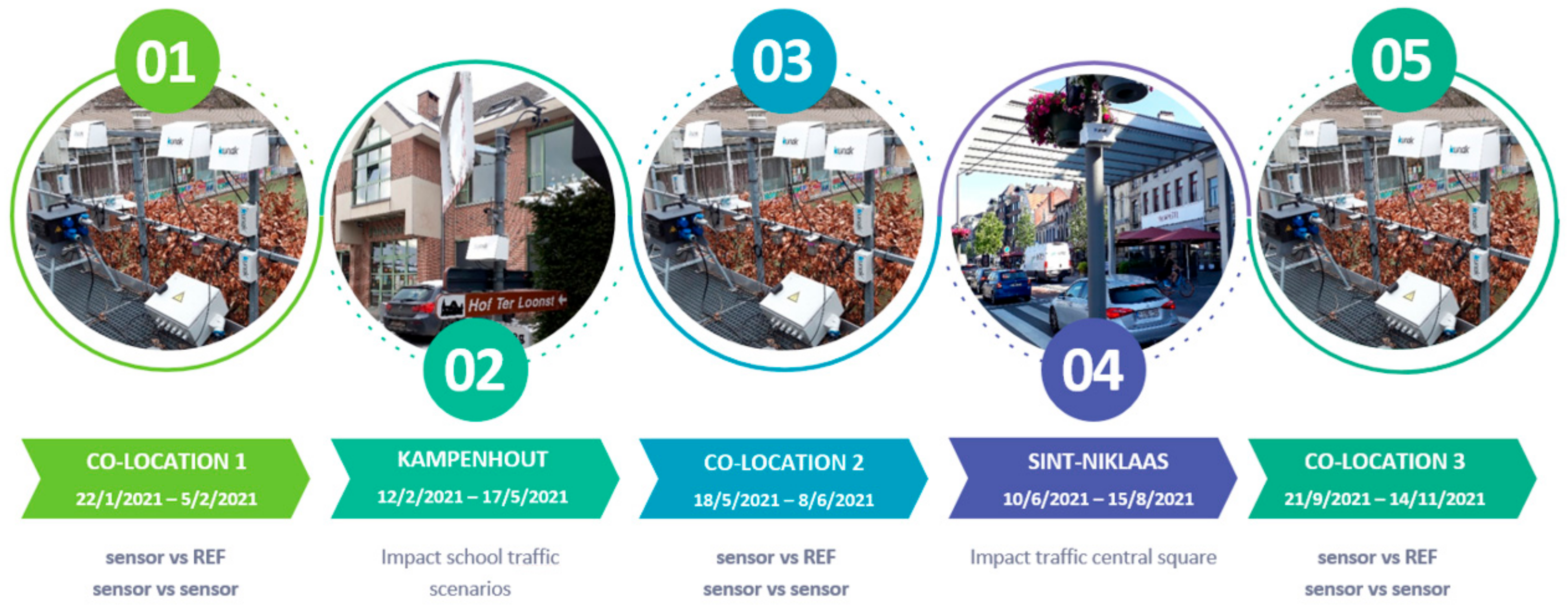
The study consisted of an initial co-location campaign of 2 weeks, co-locating all 6 sensor systems (3 of each brand/type) at an urban background air quality monitoring station (AQMS) of the Flemish Environmental Agency. After this co-location, the first pilot was conducted in Kampenhout (12 February 2021–17 May 2021). This pilot was immediately followed by a second 2-week co-location campaign (co-location 2) at the same AQMS and the second pilot study in Sint-Niklaas (10 June 2021–15August 2021). After finishing both pilot studies, we performed a final 2-week co-location campaign (co-location 3) at the AQMS (Figure 1). The recurrent co-location campaigns at a regulatory AQMS allowed for (1) performance (accuracy and precision) evaluation over time, (2) application of linear correction functions to improve sensor performance before each pilot and (3) evaluation of sensor drift and sensitivity to meteorological conditions over time.
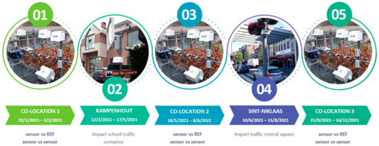
Figure 1.
Timing of subsequent benchmarking (co-location) and pilot (Kampenhout and Sint-Niklaas) campaigns during our study. Each co-location campaign evaluated the comparability between the sensors and equivalent measurements (sensor vs. REF) and intra-sensor comparability (sensor vs. sensor).
2.1. Co-Location Campaigns
During each co-location campaign, the 6 sensor units (3 Kunaks, 3 Airlys) were co-located for two weeks on the roof of a regulatory AQMS in Antwerp, Belgium (51°12′34.82″ N, 4°25′54.51″ E), near the inlets of the reference monitor for NO and NO2 (42C NO-NO2-NOx analyzer, Thermo) and equivalent (automatic) monitor for PM (FIDAS 200, Palas). In total, we considered three co-location campaigns in order to be able to compare the sensor and intra-sensor performance in different seasons and under varying environmental conditions. Moreover, potential drift or aging were considered by evaluating the accuracy over the considered time period (11 months in total).
2.1.1. Sensor Performance
We evaluated the comparability between the sensor systems and the reference (NOx) or equivalent (PM) method by calculating the following performance metrics on an hourly and daily averaging time:
- Coefficient of determination (R2): value between 0 and 1, where 1 is the best possible value. When the R2 is equal to 1, the measurements are on a perfect line, and this means that all variance in the senor data can be explained by the measured reference concentrations.
- Pearson correlation (COR): value between −1 and 1 that represents the degree of correlation between sensor and reference measurements.
- Root Mean Squared Error (RMSE): Root of the mean squared error of the measurement error between sensor and reference data; it is a frequently applied accuracy statistic and is very dependent on peaks/outliers.
- Mean Absolute Error (MAE): The mean absolute error between sensor and reference data; can be interpreted as the mean deviation between sensor and reference.
- Mean Bias Error (MBE): Mean error between sensor and reference data. This metric can be both positive and negative and represents respectively the degree of over- or underestimation of the sensor.
- Expanded Uncertainty: Measure for the uncertainty (%) around the limit or target value, as defined by the EU [65]. We calculate the non-parametric approach (Uexp), proposed by the Flanders Environmental Agency, to calculate the uncertainty near 50 µg m−3 for PM10, 30 µg m−3 for PM2.5 and 40 µg m−3 for NO2. Although both approaches aim at quantifying the sensor uncertainty near the limit value, the EU approach used in the Demonstration of Equivalence (DOE), the relative expanded uncertainty for the candidate method (Wcm) is derived from the logistic regression between sensor and reference data (model derivation), while the non-parametric approach (Uexp) is quantified experimentally (95 percentile MAE of measured concentrations within 10% range of the regulatory limit/target concentration).
In addition to the calculated performance metrics, we explored the temporal variability of the sensor and reference data using TimeVariation graphs (openair package in R [66,67]) and the sensor sensitivity to environmental conditions (temperature, relative humidity and ozone), as these variables are known to impact the performance of low-cost optical PM and electrochemical NO2 sensors [24,25,27,29,32,33,68,69,70] and need proper compensation in order to provide reliable results [25,26,28,42,45,71].
2.1.2. Intra-Sensor Performance
As the comparability between the sensor units is key to compare concentrations from multiple sensor locations against each other, the precision was evaluated by calculating the following:
- Min–Max correlation between sensor units of the same brand (Kunak, Airly);
- Min–Max MAE between sensor units of the same brand (Kunak, Airly).
2.1.3. Local Sensor Calibration
Besides evaluating the sensor performance, we explored whether a local re-calibration increased the sensor and intra-sensor performance. As the sensor systems already included calibration algorithms, we didn’t consider complex multivariate calibration models (as applied in Hofman et al. [25]), but relied on linear rescaling factors, derived from the slope of the linear regression function (intercept = 0) between the reference and sensor data, as shown in Equations (1) and (2):
where and represent the measured concentrations of the sensor and reference equipment (AQMS), respectively, and is the derived slope from the linear regression function between the raw sensor and reference data (Equation (1)). The calibrated sensor data () can subsequently be calculated by dividing the raw sensor data by the derived slope (a) from Equation (1) (Equation (2)). Former studies already showed improved performance after local re-calibration [45,46,72,73,74], as the sensor measurements are adjusted for local aerosol properties (size distribution, composition and reflectance) and environmental conditions.
2.2. Kampenhout Pilot
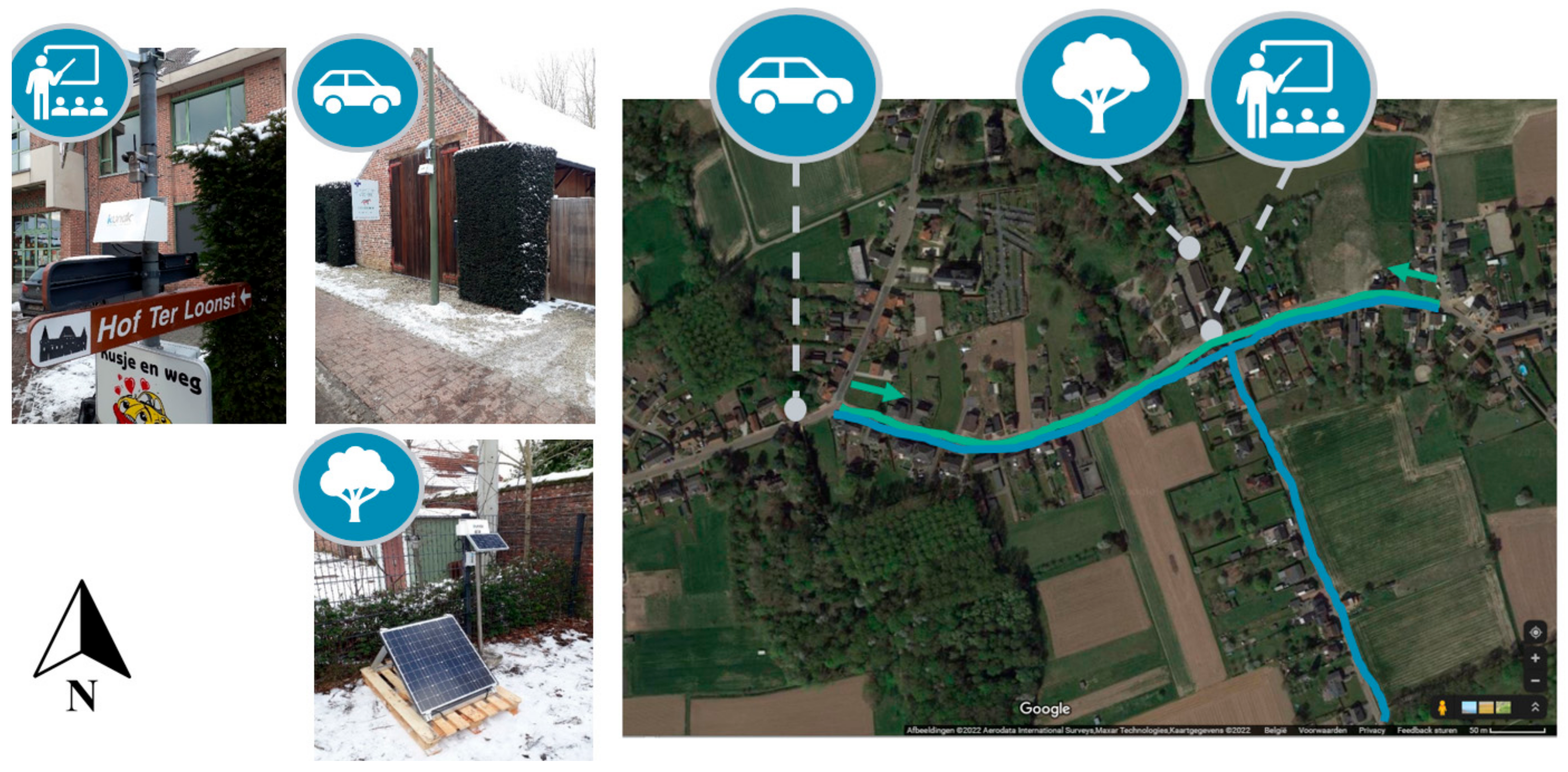
In Kampenhout, three monitoring locations were considered (Figure 2):

Figure 2.
Monitoring locations (school, environment (car), background (tree)) of the Kampenhout pilot, with associated visualizations of the Kunak and Airly deployments.
- School: Roadside location in front of the school (50°56′43.90″ N, 4°35′11.80″ E) where air quality impacts from implemented traffic measures are expected.
- Environment: Roadside location on adjacent street (50°56′41.34″ N, 4°34′51.32″ E) with similar traffic as school location and not impacted by implemented traffic measures.
- Background: Quiet location behind the school (50°56′46.16″ N, 4°35′10.46″ E) where no road traffic was present and, therefore, regarded as representative for background pollution and local sources other than road traffic.
At each monitoring location, both a Kunak and Airly unit were installed on 12 February 2021. PM, NO and NO2 concentrations were monitored for three months, until 17 May 2021. Different traffic scenarios (baseline, knip, schoolstreet) were implemented during school opening (8 h 10–8 h 40) and closing (15 h 00–15 h 45 and 11 h 00–11 h 45 on Wednesday) hours:
- Baseline scenario: No traffic restrictions, resulting in unaltered traffic flows.
- Knip scenario: one-way traffic cut in the street where the school was located (green in Figure 2), alternately in the western driving direction during school start times and the eastern direction during school end times.
- Schoolstreet scenario: 2-way traffic restriction in the street of the school and the perpendicular street (blue in Figure 2).
Each traffic scenario was implemented for about 3 weeks, while the monitoring period also included holidays (3 weeks school holidays + 1 additional week of school closure due to the COVID-19 pandemic). The timing of the implemented traffic scenarios is detailed in Supplementary Table S3. Operational performance of the sensor network (QA/QC) during the pilot was evaluated by checking the connectivity and potential operational alerts of the sensors twice a week in the online Kunak and Airly cloud dashboards.
By comparing the measured pollutant concentrations at the school location against the background location for each of the tested traffic scenarios, we were able to quantify the resulting air quality impact and identify the most optimal scenario resulting in lowest pollutant levels at the school entrance.
2.3. Sint-Niklaas Pilot
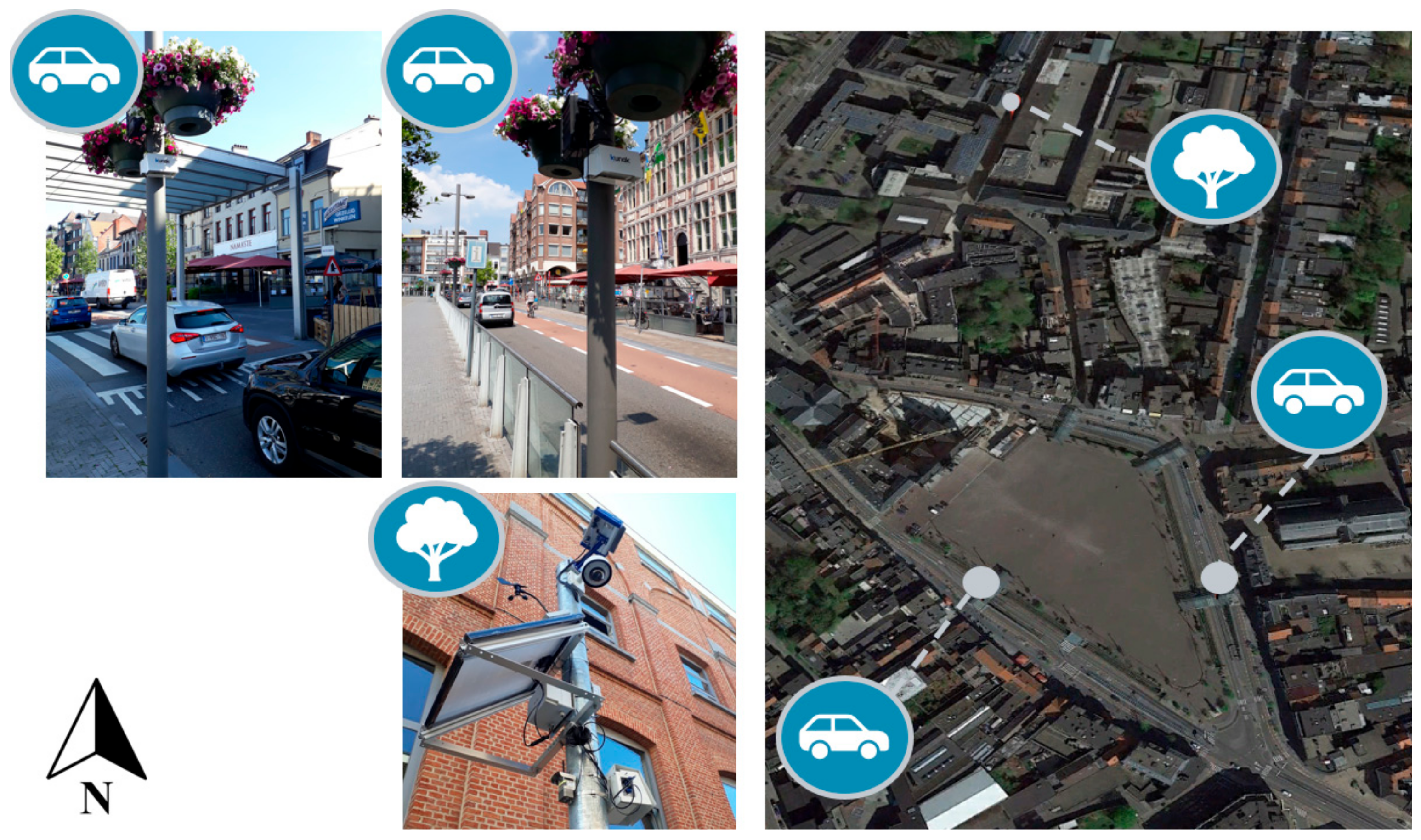
In Sint-Niklaas, three monitoring locations were considered, with one Kunak and Airly sensor unit deployed at each location (Figure 3):

Figure 3.
Monitoring locations (central city square (car) and background (tree)) of the Sint-Niklaas pilot, with associated visualizations of the Kunak and Airly deployments.
- Background: Quiet location near the main city square (51°10′1.27″ N, 4° 8′21.70″ E) in a car-free street (Paul Snoekstraat), therefore, regarded as representative for background pollution and local sources other than road traffic. Nearest (quiet) traffic was at 50 m (Collegestraat) and 40 m (Boonhemstraat).
- Grote Markt 1: Roadside location at the eastern side (Apostelstraat) of the central city square (51° 9′50.49″ N, 4° 8′28.33″ E).
- Grote Markt 2: Roadside location at the western side (Nieuwstraat) of the central city square (51° 9′50.41″ N, 4° 8′22.46″ E).
At each monitoring location, both a Kunak and Airly unit were deployed on 10 June 2021. PM, NO and NO2 concentrations were monitored for three months, until 15 August 2021. From the resulting difference between the roadside locations at the central city square (Grote Markt 1 and 2) and the background location, the local traffic-related pollution contribution was quantified for each pollutant.
Operational performance of the sensor network (QA/QC) during the pilot was evaluated by checking the connectivity and potential operational alerts of the sensors twice a week in the online Kunak and Airly cloud dashboards. By comparing the measured concentrations at the central city square locations against the background location, we were able to quantify the road traffic contribution at the central city square and potential air quality impact from future traffic restrictions.
3. Results
3.1. Co-Location Campaigns
3.1.1. Sensor Performance
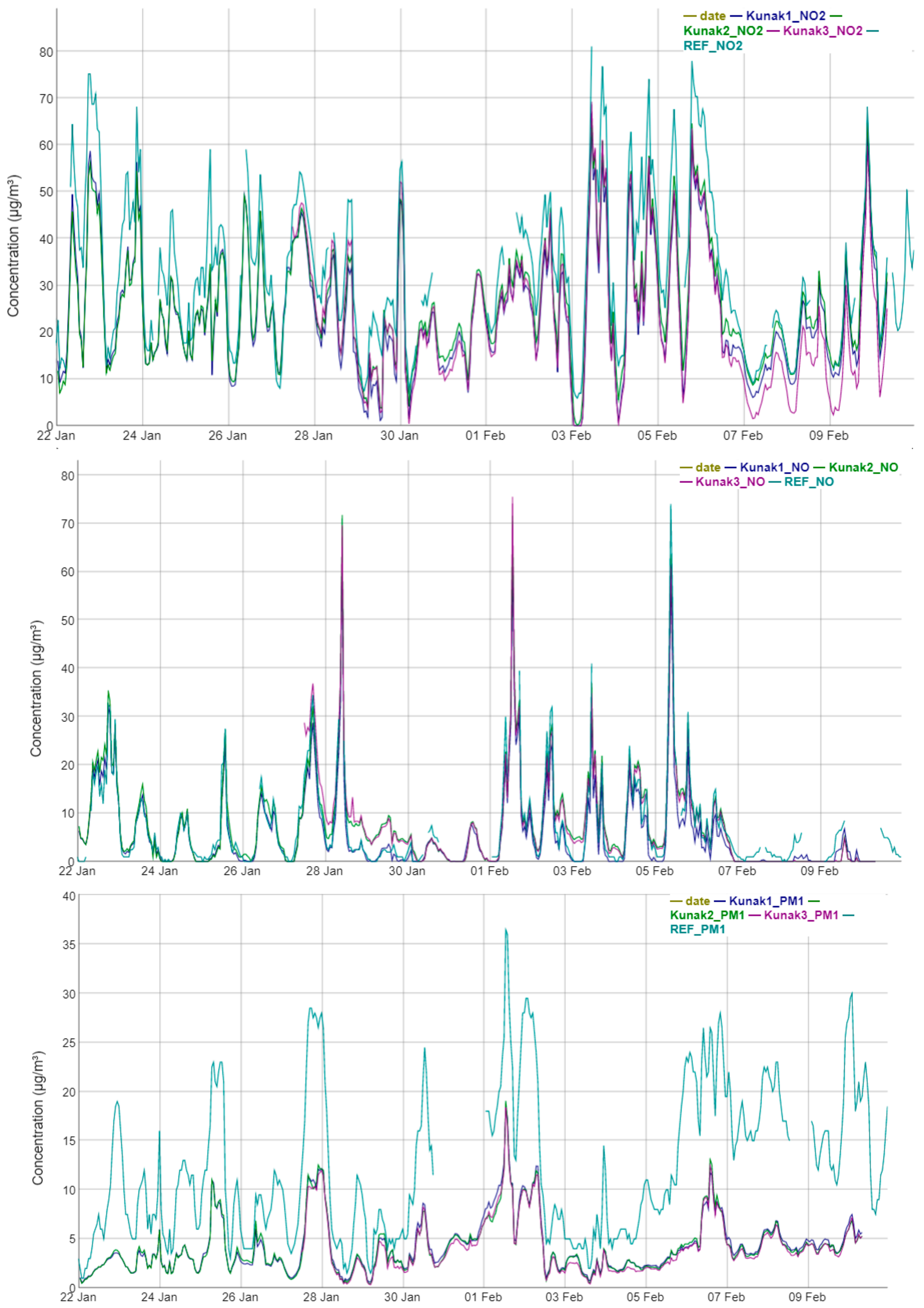
Co-location measurements (before rescaling) are visualized in timeseries graphs for the main traffic-related pollutants NO2, NO and PM1 for each of the Kunak (Figure 4) and Airly (Supplementary Table S3) sensors. From these time series, it becomes clear that the sensor measurements follow the reference measurements reasonably well, resulting in good correlations between sensor and reference data for NO2 (r = 0.96–0.97) and NO (r = 0.94–0.99) from Kunak and for PM1 (r = 0.91–0.94), PM2.5 (r = 0.89–0.92) and PM10 (r = 0.72–0.75) from Airly (Table 2), with adequate compensation for potential temperature and relative humidity effects (tested but not shown). Nevertheless, considerable under- or overestimation can be observed for some pollutants/sensors, resulting in low accuracies, e.g., for PM1 from Kunak (MAE ~9 µg/m3).
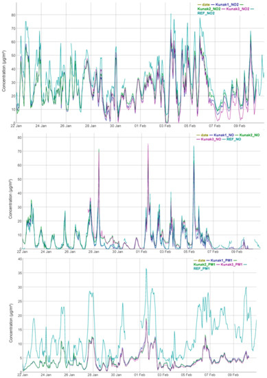
Figure 4.
Hourly-aggregated time series graphs of NO2 (upper), NO (middle) and PM1 (lower) sensor (Kunak 1–3) and reference measurements from the AQMS (42R801; REF) during the first co-location campaign (22 January 2021–10 February 2021). Similar graphs for the Airly sensors are provided in Supplementary Figure S1.
Table 2.
Data quality metrics (R², COR, RMSE, MAE, MBE, Uexp) calculated on the raw and locally re-calibrated (_cal) hourly-aggregated NO2, NO, PM1, PM2.5 and PM10 data for each of the sensor units (3 × Kunak and 3 × Airly). Local re-calibration is based on slope correction (sensor = a ∗ REF; Equation (1)), except for the NO2 of Airly (NO2_cal*) where a multilinear model was applied (sensor = a ∗ REF + b ∗ Temp + c). Uexp was only calculated for pollutants with existing limit values (NO2, PM2.5 and PM10) and, therefore, not for PM1 and NO (NA).
An overview of associated data quality metrics (R2, COR, RMSE, MAE, MBE, Uexp) for co-location campaign 1 based on hourly values is presented for NO2, NO, PM1, PM2.5 and PM10 in Table 2. The same statistics were also calculated on daily-aggregated data and are provided in Supplementary Table S4. Table 2 shows data quality metrics (R2, COR, RMSE, MAE, MBE, Uexp) calculated on the raw and locally re-calibrated (_cal) hourly-aggregated NO2, NO, PM1, PM2.5 and PM10 data for each of the sensor units (3 × Kunak and 3 × Airly). Local re-calibration is based on slope correction (sensor = a ∗ REF; Equation (1)), except for the NO2 of Airly (NO2_cal*), where a multilinear model was applied (sensor = a ∗ REF + b ∗ Temp + c). Uexp was only calculated for pollutants with existing limit values (NO2, PM2.5 and PM10) and therefore not for PM1 and NO (NA).
As both the Airly and Kunak unit hold the same electrochemical NO2 sensor (Alphasense NO2-B43F), it was quite surprising to see the difference in sensor performance (similar over the multiple co-location campaigns), probably related to differences in the applied property algorithms to calibrate the sensors and compensate for environmental impacts. The better PM performance observed for the Airly units can be explained by either the difference in PM sensors (PPMS5003 (Plantower, Beijing, China) vs. OPC-N3 (Alphasense, Essex, UK)) or the associated calibration and compensation algorithms.
3.1.2. Intra-Sensor Performance
From Figure 4, low intra-sensorvariability (precision of the sensor units) can be observed, which is very important for the intended purpose of our pilots, since we want to compare different sensor units (locations) against each other. Good intra-sensor performance was confirmed when calculating the Min–Max correlation and MAE between the considered sensor units (Table 3), showing that the agreement between the sensor units is better than the agreement between the sensor and reference measurements. Moreover, correlations and MAEs were also similar between the three co-location campaigns (Table 3), meaning that intra-sensor performance does not deteriorate over the considered time period (11 months).
Table 3.
Minimum and Maximum Pearson correlations (COR) and Mean Absolute Errors (MAEs) between the considered sensor units for NO2, NO, PM1, PM2.5 and PM10 before (RAW) and after (CAL) local re-calibration.* During the final co-location, only two Airly sensors were available.
3.1.3. Local Re-Calibration
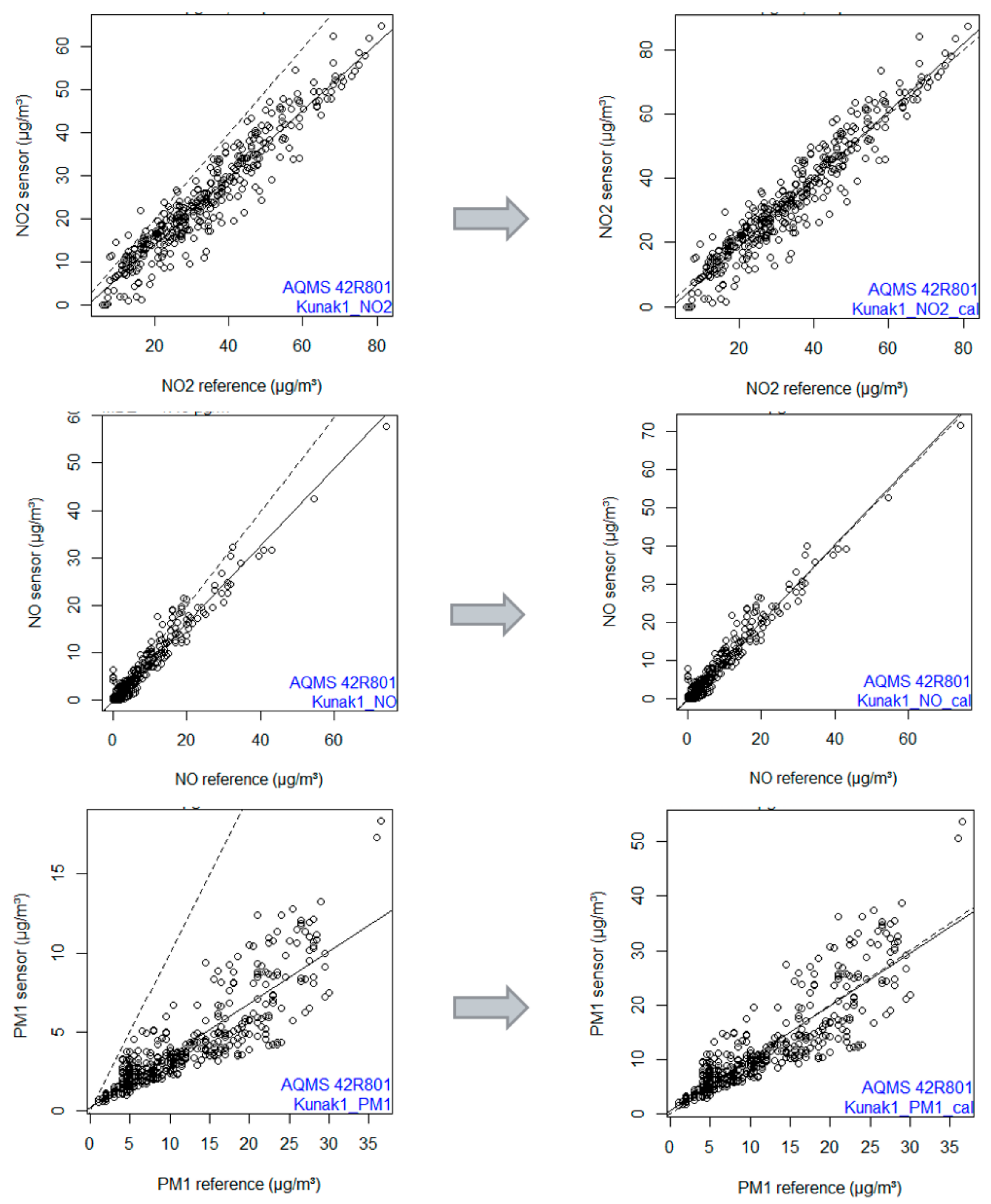
As the linear correlations between the sensor and reference data were generally good (mostly r > 0.9) and did not exhibit temperature and/or relative humidity effects (not shown) for NO2 and NO (Kunak) and PM1, PM2.5 and PM10 (Airly), and a significant amount of residual variation can be explained by the slope, slope calibration factors were implemented as explained in Section 2.1.3 and shown in Figure 5. We derived slope calibration factors for each pollutant and sensor and calculated the sensor performance again based on the re-calibrated sensor data (“_cal” in Table 2). This exercise resulted in an improved accuracy (RMSE, MAE, MBE, Uexp) for all pollutants and sensors and similar correlations (R2 and COR), as can be seen from Table 2 and Supplementary Figure S2. While the expanded uncertainty of the original sensor data did not reach the data quality objectives (DQOs) for indicative measurements (50% for PM, 25% for NO2) as defined at the EU level [65], the DQOs were met after slope re-calibration for Airly PM2.5 and PM10 and Kunak PM10 (<50%) and approximated for Kunak NO2 (~25%), as can be seen from Table 2.

Figure 5.
Effect of the local slope re-calibration on NO2 (upper), NO (middle) and PM1 (lower) data from Kunak 1 during co-location campaign 1. The recalibrated data (right) approximates the 1:1 line (dashed) much better when compared to the raw sensor data (left). Regression plots for all considered pollutants of both Konak and Airly are provided in Figure S2.
This re-calibration approach based on slope factors improved the sensor performance for all pollutants/sensors, except for the Airly NO2, where an additional sensitivity towards atmospheric temperature (°C) was observed (Supplementary Figure S3). By considering a multilinear re-calibration model compensating for both slope and temperature (covariates), we were able to explain the residual variability and improve the sensor performance (Supplementary Figure S3). This was, however, out of scope for this study, as we wanted to evaluate out-of-the-box performance and added value of easily-derived calibration factors for the local user communities.
In conclusion, the considered sensor systems generally performed quite well and followed the pollutant dynamics of the reference measurements. Nevertheless, a local calibration (rescaling) is advisable to improve the sensor accuracy. While Airly performs best for PM, Kunak gives the best results for NO2 and NO. Note that the evaluation is based on sensor system versions available at the time of the study, and improvements of newer versions can be expected. After implementing the local re-calibration factors, we reached overall good performance for Kunak NO2 (R2 = 0.92–0.95, MAE = 3.38–4.67 µg m−3) and NO (R2 = 0.88–0.98, MAE = 1.2–2.77 µg m−3) and Airly PM1 (R2 = 0.82–0.87, MAE = 2.16–2.33 µg m−3) and PM2.5 (R2 = 0.79–0.92, MAE = 1.11–3.1 µg m−3). Taking into account the observed data quality and the implemented policy measures (traffic restrictions) in Kampenhout and Sint-Niklaas, further data analysis of the pilots will focus on the best performing sensor systems for traffic-related pollutants NO (Kunak), NO2 (Kunak) and PM1 (Airly).
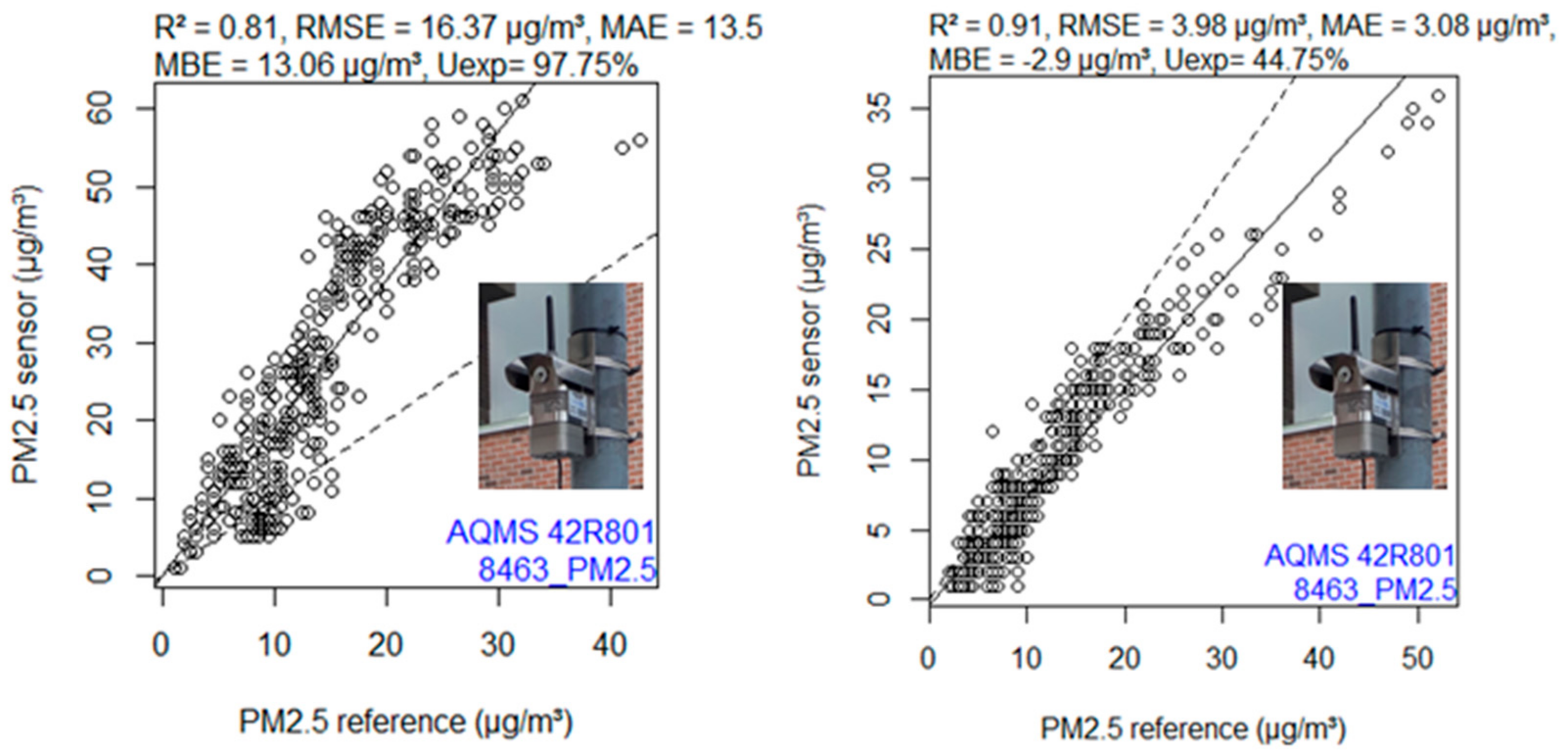
When comparing the sensor performance (Supplementary Table S6) and derived slope factors (Supplementary Table S5) between the recurrent co-location campaigns, it becomes clear that both the raw sensor performance and derived slopes tend to vary throughout the year. The raw NO2 sensor performance reduces in the summer period (second co-location), possibly due to impacts from temperature and ozone, while PM performance decreases during the winter first and third co-location), probably related to a higher relative humidity. While the raw PM sensor readings underestimated PM concentrations during the summer (co-location 2), they overestimated PM concentrations during the winter (co-locations 1 and 3), as can be seen from Figure 6.
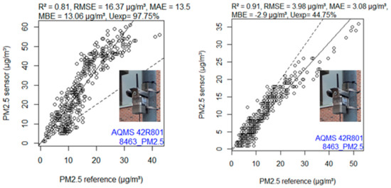
Figure 6.
Regression plots of Airly PM2.5 raw sensor readings against reference data during a winter (1; left) and summer (2; right) co-location campaign. Associated performance metrics (R2, RMSE, MAE, MBE and Uexp) are provided above the plots.
This seasonal variation of environmental parameters, therefore, tends to impact the sensor performance. However, after applying the slope re-calibration, similar sensor performances are achieved to the first co-location period (Supplementary Table S6), indicating that (1) recurrent co-location calibrations can cope with changing environmental impacts and (2) no significant sensor aging or drift is observed in the considered study period (11 months).
3.2. Kampenhout Pilot
3.2.1. Descriptive Statistics and Temporal Variability
As described in Section 2.2, PM, NO and NO2 concentrations were monitored at three locations (background, school and environment) between 12 February 2021 and 17 May 2021. Slope re-calibration factors from the preceding co-location campaign (co-location 1 in Supplementary Table S5) were applied to the sensor data, and descriptive statistics of the exhibited pollutant concentrations and meteorological conditions (temperature, relative humidity and pressure) are provided in Supplementary Table S7. Data coverage during the pilot was good (>95%), and meteorological conditions were very similar between the considered locations. This is not surprising, as all locations are located within a 400 m radius.
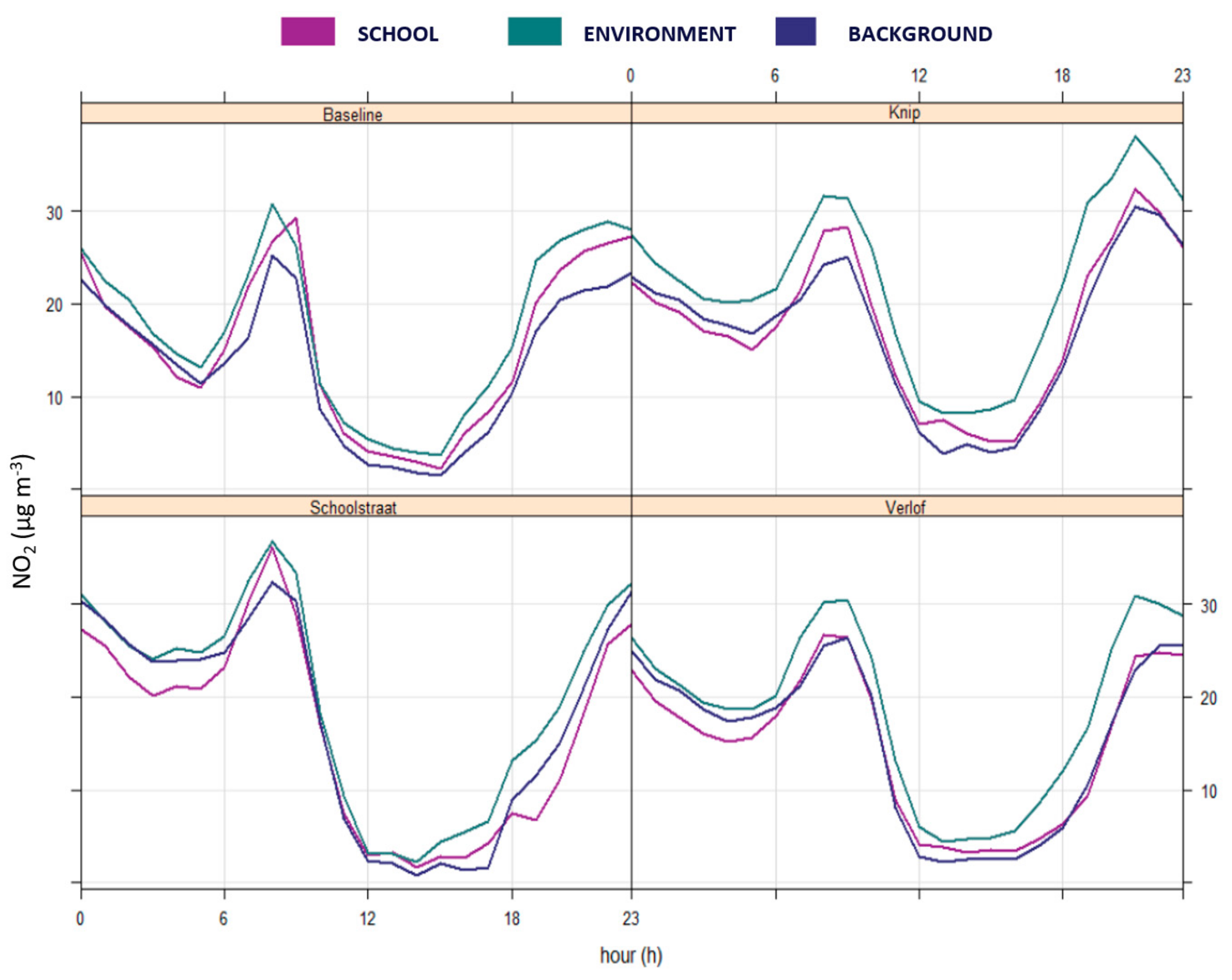
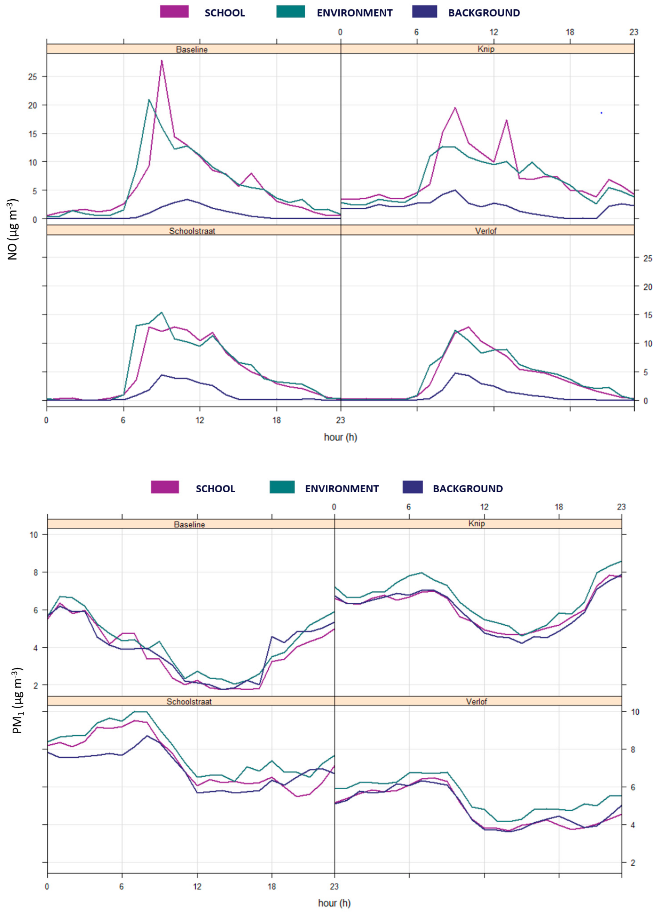
Time series graphs in Supplementary Figure S4 show realistic concentration dynamics throughout the monitoring campaign, and diurnal pollutant variability with distinct morning and evening rush hour peaks were observed for NO2, NO and PM1 (Figure 7). From the diurnal pattern of the monitoring locations and the implemented traffic scenarios, it becomes clear that similar pollutant dynamics are observed at all monitoring locations, with highest concentrations at the environment location (roadside, not impacted), followed by the school location (roadside, impacted) and the background location (no traffic). During school start times, concentration differences between the background and school location are highest for NO (16 µg m−3), followed by NO2 (4 µg m−3) and are only moderate for PM1 (<1 µg m−3). This can be explained by the fact that NO is emitted by traffic and rapidly oxidizes to NO2. NO can, therefore, be regarded as a short-lived pollutant, resulting in steep concentration gradients near roads (difference in background vs. school/environment location in Figure 7). The NO2 concentrations result from primary emissions and converted NO. NO2 can be transported over longer distances, and the ratio of NO/NO2 is the result of a complex photochemistry, resulting in a less direct relation of NO2 to traffic compared to NO. PM is predominantly influenced by background pollution and can be generated by a wide range of direct and indirect emission sources.
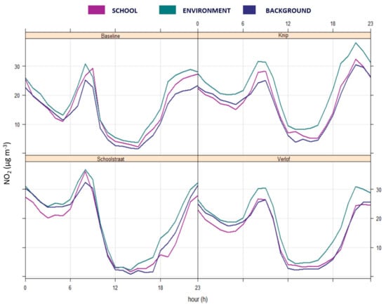
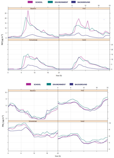
Figure 7.
Average hourly NO2 (upper), NO (middle) and PM1 (lower) concentration (µg m−3) variability throughout the day (0–23 h), plotted for each monitoring location (school, environment and background) and implemented traffic scenario (baseline, knip, schoolstreet and school holidays (verlof)).
During school start (8–9 h) and end (15–16 h) times, increased NO and NO2 pollutant concentrations at the school location are observed in Figure 7, most clearly during the baseline (no traffic restriction), to a lesser extent during the knip scenario (one-way traffic restriction) and to a negligible extent during the schoolstreet scenario and holiday periods. For PM1, it is hard to observe any difference in concentrations between the scenarios based on the diurnal graphs (Figure 7). Lowest overall NO2, NO and PM1 concentrations are observed during the school holiday periods. Although these observations already suggest an air quality impact from the implemented traffic scenarios, actual scenario differences are calculated in Section 3.2.2.
3.2.2. Traffic Scenario Differences
As the traffic scenarios were only implemented on weekdays (n = 1776), during school start and end times (n = 161), we extracted this data from the overall hourly-aggregated dataset. When comparing the observed pollutant variability of these data subsets between the traffic scenarios (baseline, knip, schoolstreet) and holiday periods at the school location using boxplots and Wilcoxon Rank significance tests (Supplementary Figure S5), significant concentration differences were only observed for NO. However, scenario differences were mimicked due to the varying background concentration. Higher background concentrations were observed for NO2 (+28%), NO (+44–66%) and PM1 (+123–185%) during the implemented traffic scenarios, when compared to the baseline scenario (Supplementary Figure S6). In order to take into account background concentration variability, we normalized the school location concentrations using the concentrations observed at the background location, both absolute (µg m−3; Equation (3)) and relative (%; Equation (4)), for comparison:
where is the normalized concentration (µg m−3), is the hourly-averaged pollutant concentration measured at the school location (µg m−3) and is the hourly-aggregated concentration simultaneously measured at the background location (µg m−3). can, therefore, be regarded as the local pollution contribution at the school location.
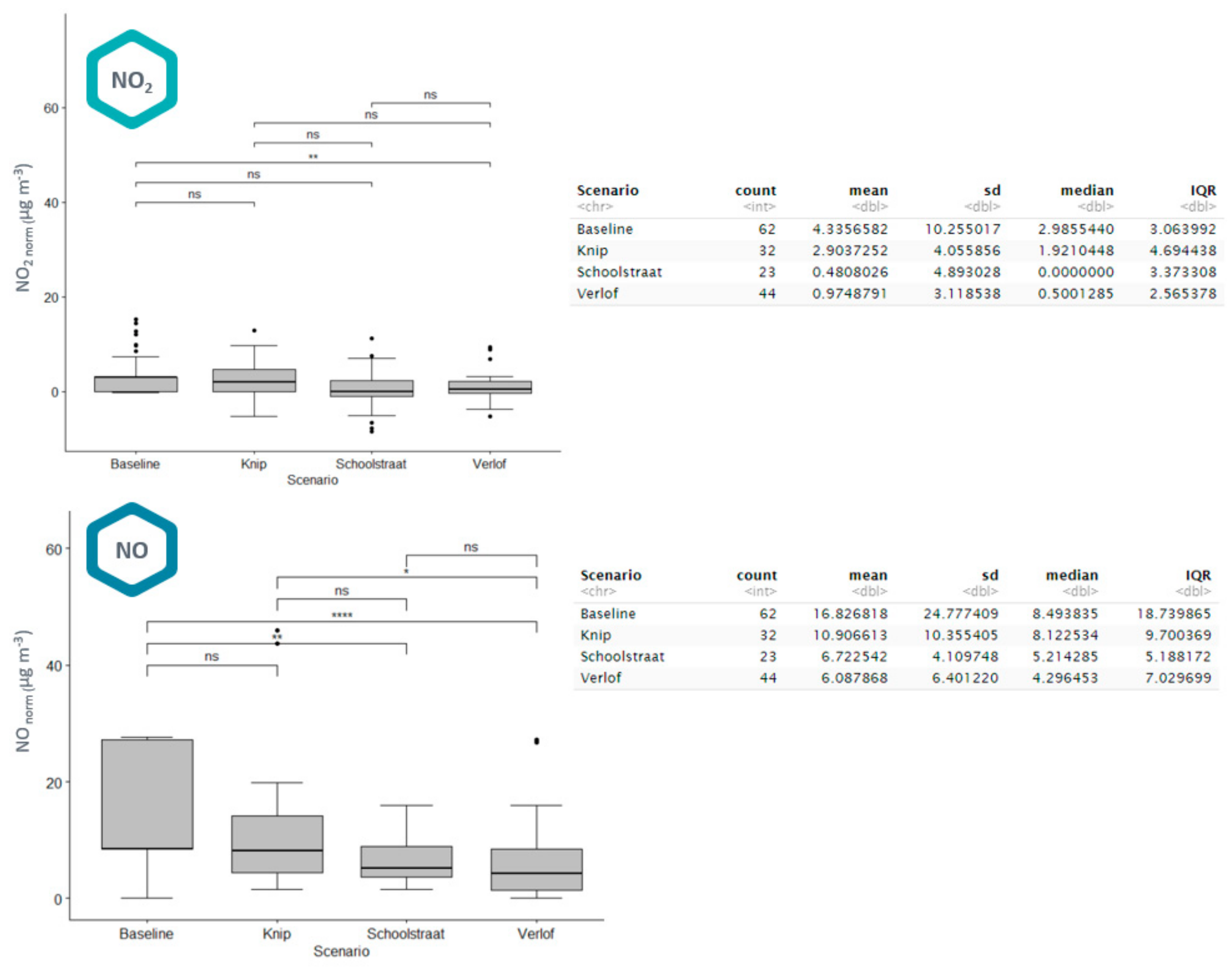
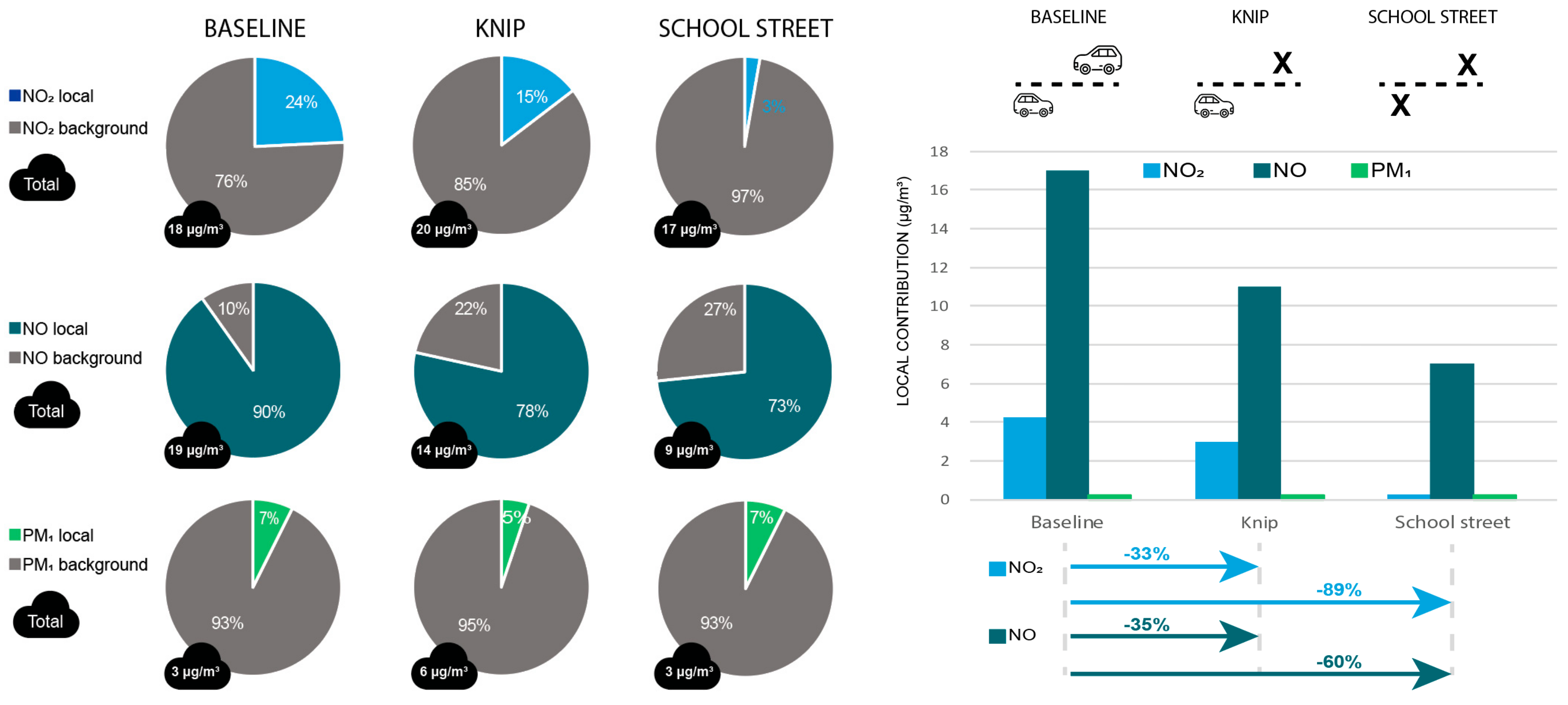
Based on the resulting boxplots and descriptive statistics of the normalized pollutant concentrations () in Figure 8, we can state that the average local NO2 contribution (during the scenarios; 8–9 h and 12–13 h/15–16 h) decreases from 4.33 µg m−3 (baseline) to 2.9 µg m−3 (−33%) during the knip scenario (one-way traffic restriction) and to ~0.5 µg m−3 (−89%) for the schoolstreet scenario (two-way traffic restriction). For NO, the air quality impact is even more significant, from 16.83 µg m−3 (baseline) to 10.91 µg m−3 (−35%) for the knip scenario and 6.72 µg m−3 (−60%) for the schoolstreet scenario. Finally, for PM1, we see no effects on the scenarios, with a negligible local PM1 contribution at the school location (0.06–0.31 µg m−3). The observed concentration differences between the traffic scenarios exceed the intra-sensor uncertainties quantified in the co-location campaigns (Table 3), and can therefore be explained by the implemented traffic scenarios.

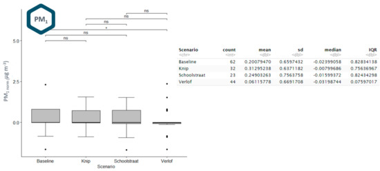
Figure 8.
Boxplots with associated Wilcoxon Rank scores (*: p < 0.05, **: p < 0.01, ****: p < 0.001) for the local contribution of NO2 (upper), NO (middle) and PM1 (lower) exhibited at the school location during school opening/closing hours (n = 161). Associated descriptive statistics (n, mean, standard deviation (sd), median and interquartile range (IQR)) are provided next to each plot.
3.3. Sint-Niklaas Pilot
As described in Section 2.3, PM, NO and NO2 concentrations were monitored at three locations (background, Grote Markt 1 and 2) between 10 June 2021 and 15 August 2021. Slope re-calibration factors derived from the preceding co-location campaign (co-location 2 in Supplementary Table S5) are applied to the sensor data. The resulting average pollutant concentrations for NO2, NO, PM1, PM2.5 and PM10 are provided in Table 4. Data coverage during the pilot was again very good (>95%), as can be seen from the time series graphs in Supplementary Figure S7.
Table 4.
Average NO2, NO, PM1, PM2.5 and PM10 concentrations exhibited during the pilot campaign in Sint-Niklaas.
The average NO and NO2 concentrations are clearly higher at the central city square locations (Grote Markt 1 and 2), when compared to the background location (up to 6 µg/m3 higher for NO2 (+50%) and up to 8 µg/m3 higher for NO (+360%)). For PM1, a modest concentration increase of 2.5 µg m−3 (+8%) compared to the background location is only observed at one of the Grote Markt locations (Grote Markt 1). The location differences for NO and NO2 are larger than the observed uncertainty between the sensors (Table 3) and should, therefore, be explained by effective location differences. Considering traffic as an important source of NO and NO2 (confirmed in the Kampenhout pilot) and the car-free background location, our results indicate that increased traffic emissions at the Grote Markt locations give rise to elevated atmospheric NO and NO2 concentrations.
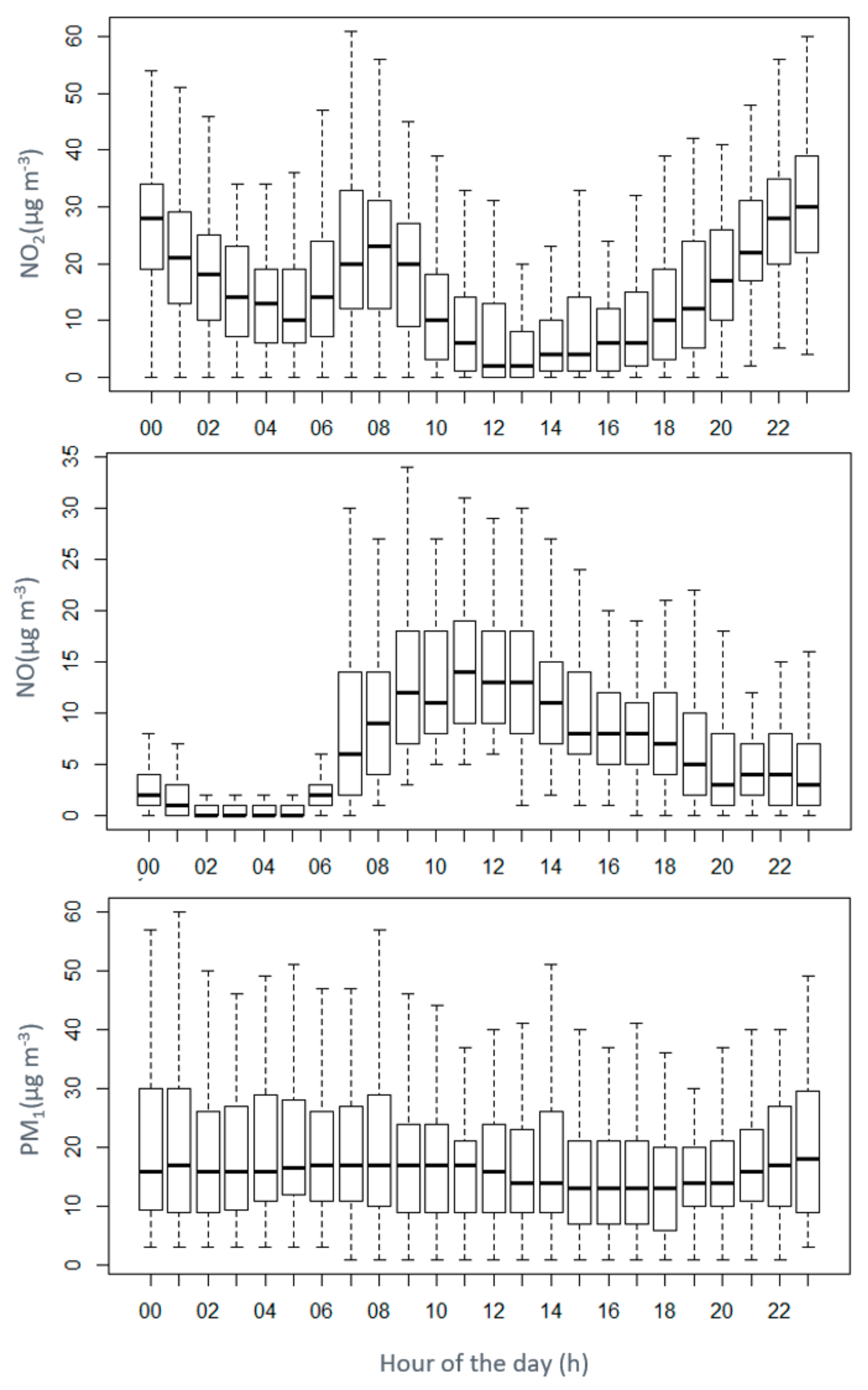
When evaluating the hourly pollutant variability at the central square (Figure 9), higher morning and evening rush hour peaks are observed for NO2. From midday onwards, NO2 reacts with O2 (+UV and heat), forming NO and O3 and decreasing NO2 concentrations. This photochemical balance is inversed in the late evening, when an excess of NO from the evening rush hour peak (in absence of UV from solar radiation) reacts with O3, forming NO2 again. From 23 h onwards, NO2 concentrations are reduced due to the absence of direct emissions. As direct NO emissions from traffic are very short-lived (rapid oxidation towards NO2) and NO is only formed under sunny conditions, nighttime NO concentrations are very low. The diurnal pattern of NO2 and NO is, therefore, impacted by both direct emissions and photochemical reactions between NOx and ozone. Hourly PM variability at the central square is very low, as can be seen from Figure 9. Hourly-averaged NO2 and NO concentrations at each monitoring location are provided in Supplementary Figure S8 and show the most distinct location differences for NO, followed by NO2.
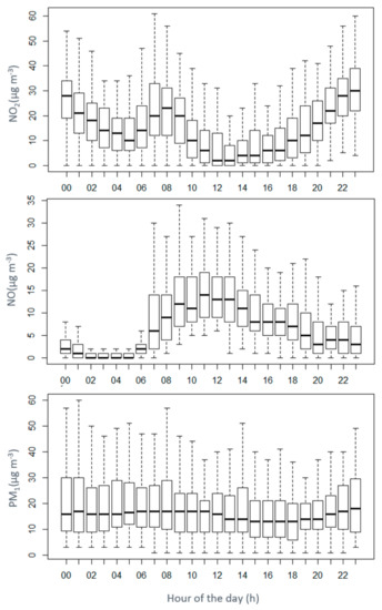
Figure 9.
Hourly NO2 (Kunak; upper), NO (Kunak; middle) and PM1 (Airly; lower) variability as observed at the Grote Markt 1 location.
To focus on the actual traffic contributions at the central square (Grote Markt), we calculated normalized pollutant contributions during the morning rush hour (6–9 h), following Equation (3). Local pollutant contributions (difference between background and central square locations) during the morning rush hour amounted to ~8.4 µg m−3 for NO2 (+30%), ~11.7 µg m−3 (+180%) for NO and 1–2 µg m−3 (+5%) for PM1. This effect was pronounced for NO2 (+43%) and NO (+216%) when only considering working days and dropped to ~0% during the weekends, which confirms our traffic hypothesis. Observed air quality impacts again exceeded between-sensor uncertainties for NO and NO2, which confirms that observed air quality impacts are due to location differences.
4. Discussion
4.1. Data Quality
The considered sensor systems generally performed quite well in terms of data capture (>95%), correlation and intra-sensor uncertainty. However, good out-of-the-box accuracy was not guaranteed, and a local calibration (rescaling) seems advisable to improve the sensor accuracy to supplementary levels (<50% for PM and <25% for NO2). Performance was related to both hardware setup (applied sensors) and applied compensation and calibration property algorithms, with Airly performing best for PM and Kunak giving the best results for NO2 and NO. After implementing the local re-calibration factors, we reached overall good performance for Kunak NO2 (R2 = 0.92–0.95, MAE = 3.38–4.67 µg m−3) and NO (R2 = 0.88–0.98, MAE = 1.2–2.77 µg m−3) and Airly PM1 (R2 = 0.82–0.87, MAE = 2.16–2.33 µg m−3) and PM2.5 (R2 = 0.79–0.92, MAE = 1.11–3.1 µg m−3). While the expanded uncertainty of the original sensor data did not reach the data quality objectives (DQOs) for supplementary measurements (50% for PM, 25% for NO2), as defined at the EU level [65], the DQOs were met after slope re-calibration for Airly PM2.5 and PM10 and Kunak PM10 (<50%) and were approximated for Kunak NO2 (~25%). High intra-sensor precision was observed for both Kunak and Airly. This is important, as many sensor use cases (like the Kampenhout and Sint-Niklaas pilots) rely on comparisons of multiple monitoring locations (between sensor units).
Although the sensor price range was not necessarily indicative of the data quality (Airly PM performed better than Kunak PM), the more costly Kunak sensors offered much more flexibility, local calibration and configuration options, more data monitoring tools with dedicated warnings (e.g., flow PM sensor), extended analytics based on the statistical openair package [67] and availability of governmental air quality monitoring stations in their cloud dashboard. In contrast, the Airly sensors and interface are more basic, but the price of these sensors is ~10 times lower.
Field co-location campaigns seem vital to (1) evaluate and improve the performance of contemporary sensor systems against actual reference equipment and (2) quantify intra-sensor uncertainty for proper interpretation of the sensor data during their implementation (locations differences > instrument noise). In addition, we noticed that environmental impacts changed throughout the year, resulting in varying re-calibration factors for the three co-location campaigns. Ideal calibration should, therefore, be repeated, e.g., by conducting recurrent co-locations (e.g., every 3 months, at least at locations with large seasonality) [26], as applied in our study. Other (re-)calibration approaches that are proposed in the literature include (1) continuous scaling of co-location-derived calibration factors to a deployed sensor network [44,74,75], (2) distant calibration of sensors based on the existing reference network [25,54,76] or (3) a combination of field and mobile calibration approaches [42].
4.2. Pilots
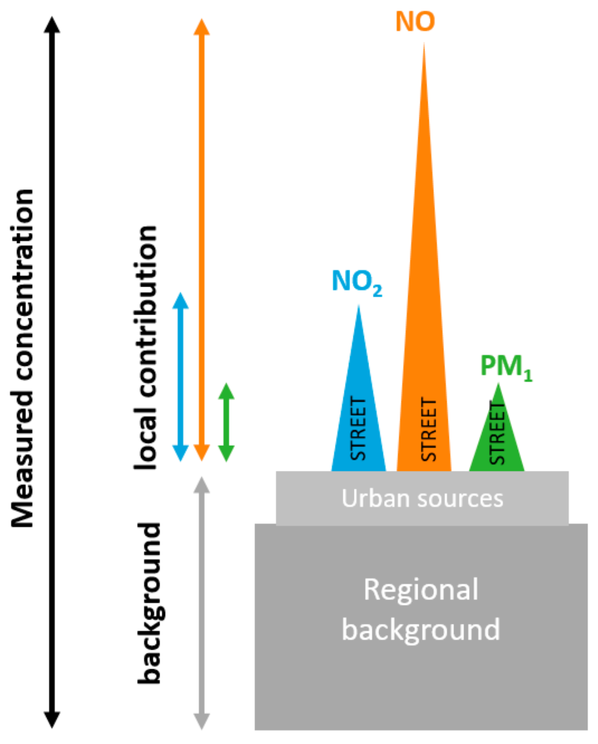
When considering policy measures to improve local air quality (e.g., via traffic measures), it is important to think about the general build-up of air pollution in cities. Urban air pollution consists of background contributions from cross-boundary, regional and urban sources and local contributions from nearby sources, i.e., traffic (Figure 10). The maximum achievable air quality improvement from local measures is therefore the local contribution, which, at the roadside, showed to be the highest for NO, followed by NO2 and PM. The use of background monitoring locations proved to be very valuable, as we experienced background concentration fluctuations mimicking the impacts from the implemented traffic measures in one of the pilots (Kampenhout). By considering both a local source and background monitoring location simultaneously, measured concentrations at the source location can be normalized continuously for fluctuating background concentrations. This allows for quantification of (1) the local source contribution (= maximum potential air quality impact of local interventions), and (2) resulting air quality impacts from short-lived traffic interventions (e.g., one-way cut and school street).

Figure 10.
Urban air pollution buildup with contributions from background and local sources for NO2 (blue), NO (orange) and PM1 (green).
Although the sensor locations were fairly close to each other (<400 m), quantifiable location differences were observed in both pilots, exceeding the intra-sensor uncertainty quantified in the co-location campaigns. We can therefore state that the considered sensor systems were able to detect air quality impacts from local traffic in front of a school in Kampenhout and at a central city square in Sint-Niklaas. The local traffic-related pollution contribution (potentially impacted by local traffic measures) in Kampenhout was the highest for NO (90%), followed by NO2 (24%), and was only negligible for PM1 (~7%) (Figure 11). In Sint-Niklaas, similar findings were observed with the local rush hour contributions of NO2 and NO (Supplementary Figure S9). This is important information, as it shows the maximal achievable air quality impacts from local policy measures. In Kampenhout, implemented traffic measures (knip, school street) resulted in a reduction of this local pollution contribution of up to 89% for NO2 and 60% for NO (Figure 11). Both pilots thus support the use of local traffic measures to improve local air quality in cities.
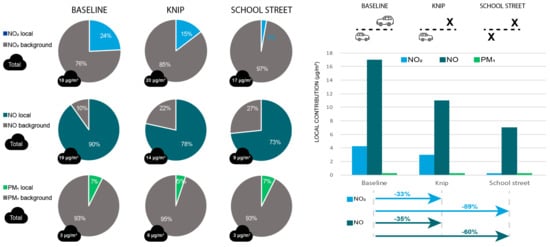
Figure 11.
(Left panel): local and background NO2, NO and PM1 contribution during baseline (left), knip (middle) and school street (right) scenario. (Right panel): Absolute and relative (%) impacts from knip and school street scenarios on local NO2, NO and PM1 contributions.
As we only considered a limited monitoring period in our pilots, 3 months (~3 weeks/traffic scenario) in Kampenhout and 2 months in Sint-Niklaas, and seasonal dynamics in air quality and modal split likely influenced the observed traffic scenario impacts, generalization of the observed results is difficult.
Nevertheless, our results seem to confirm the few existing studies reporting air quality impacts from traffic management scenarios near school environments and urban environments in general. A recent intervention study on the impact from traffic restrictions (school streets) at three schools (high-end instruments) in Belgium reported decreased morning rush hour peaks for NO2, BC and UFP by comparing concentrations during the traffic intervention (school street) with concentrations from the hour before the intervention [61]. Results showed that the implemented traffic restrictions resulted in an average (morning drop-off) concentration decrease for NOx (from +32 to +77% (pre-) to −23% to +22% (post-intervention)), BC (from +18 to +58% (pre-) to −27% to +38% (post-intervention)) and UFP (from +15 to +19% (pre-) to -9% to +8% (post-intervention)) [61]. Another study with 30 AQMesh sensors at 16 schools in London (UK), comparing schools with traffic restrictions (school street) against schools without traffic restrictions [77], reported average reductions in nitric oxide (NO) concentrations of up to 8 µg/m3 (34%) during the morning intervention period, which equates to a reduction in daily average (school day) concentration of approximately 5%. The resultant reduction in nitrogen dioxide (NO2) during the school drop-off period was estimated as being up to 6 µg/m3 (23%). The morning intervention alone was thus expected to reduce daily average NO2 by up to 0.4 µg/m3, or 2%. Moreover, 81% of parents and carers supported the measures at their children’s school, and 18% of parents reported driving to school less as a result of school streets [77]. In terms of the local pollution contribution from road traffic, a recent study with mobile sensors on buses in Hong Kong, determining local and background contributions for NO, NO2, CO and PM2.5, showed that NO and NO2 are locally dominated air pollutants, constituting 72%–84% and 58%–71%, respectively, whereas PM2.5 and CO largely arise from background sources, which contribute 55%–65% and 73%–79%, respectively [78]. Another recent study showed the distinct traffic-related impacts from the COVID-19 lockdown in the United Kingdom on resulting NO2 and NO concentrations, with observed concentration reductions of 32 to 50% at urban traffic stations and 26 to 46% at urban background stations, while no concentration reductions (or even increases) were observed for O3 and PM [59].
Although these studies are all different in terms of implemented traffic interventions (traffic restriction, cut, lockdown, etc.), applied instrumentation (sensors vs. monitors, fixed vs. mobile deployments) and data analysis (normalized based on previous hour [61], normalized based on simultaneous background concentration (our study), normalized based on locations without traffic interventions [77]) and consider different time periods and/or pollutants, there seems to be common evidence that road traffic results in local pollution contributions (NO>NO2>PM), and local air quality improvements can be expected from when implementing traffic interventions.
4.3. Blueprint for Urban Air Quality Sensor Networks
A total of 79 Belgian municipalities and cities and the Flanders Environmental Agency (VMM) contributed in the research trajectory towards the usability of commercial air quality sensor systems for evidence-based policy making. This trajectory included a literature search and market analysis [64], workshops and survey on the needs and requirements, problem statement, functional properties, and visualization and communication aspects of air quality sensors. After a preparatory phase, the above pilot sensor networks were deployed to address the real-world policy concerns of local authorities. Based on the feedback from the involved cities, sensor data were deemed useful as an evidence base for planned policy measures and were communicated to citizens. The involved municipalities and cities indicated that organizing air quality sensor networks at the local municipal level is still challenging, with sensor selection, data quality evaluation and data analysis as the most challenging processes, requiring support from external experts or agencies.
To this end, we developed a hands-on tool (blueprint) for local governments aiming to roll out air quality sensor networks in their municipality or city. The blueprint includes scoping advice and practical tools (e.g., sensor selection tool) with regard to the entire design process, including defining a research question, experimental setup, roll out, data analysis and communication (Figure 12). This blueprint is available online [79].
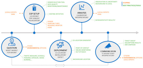
Figure 12.
Blueprint for a municipal air quality sensor network. Scoping (orange) and best practices (green) based on real-world experiences are given for each step in the design process.
5. Conclusions
This work describes a collaborative effort of a research institute (VITO), local authorities and the regional environmental agency (VMM) in substantiating local air quality policies with actionable sensor data from commercially available air quality sensor systems (Airly, Kunak). The aim was to evaluate the usability of commercial “low-cost” air quality sensor systems to substantiate evidence-based policy making by quantifying the local pollution contribution from road traffic at a central city square and potential impacts from different traffic measures in a school environment.
Both pilots demonstrate that contemporary air quality sensors are able to accurately quantify air quality impacts from (even short-lived) local traffic measures and contribute to evidence-based policy making, under the condition of a proper methodological setup (background normalization) and data quality (recurrent calibration) procedure. When considering commercially available sensor solutions, co-location campaigns remain vital to benchmark the data quality of the sensors, evaluate the validity of observed effects (sensor precision) and improve sensor performance through calibration. Including a local background location in the sensor network has proven methodologically valuable to normalize for background pollutant dynamics and to quantify local pollutant contributions (i.e., potential impact of local policy measures). Based on the feedback from the involved cities, sensor data were deemed useful and can empower local authorities to implement new air quality management plans. To this end, a blueprint was developed to help local authorities in setting up local air quality senor networks.
Supplementary Materials
The following supporting information can be downloaded at: https://www.mdpi.com/article/10.3390/atmos13060944/s1. Table S1. Comparison of defined functional requirements (Table 1) against specifications from commercially available sensor systems. Table S2. Sensor specifications of the considered Kunak Air A10 and Airly PM+Gas sensors, derived from AQMD AQ-SPEC (http://www.aqmd.gov/aq-spec/home); Table S3. Timing of the implemented traffic scenarios (baseline, knip and schoolstreet) and holiday periods during the pilot study in Kampenhout; Figure S1. Hourly-aggregated time series graphs of NO2 (upper) and PM1 (lower) from the different Airly units (8463, 12,744 and 12,798) and refer-ence measurements from the AQMS (42R801; REF) during the first co-location campaign (22 January 2021–10 February 2021). The Airly sensors do not contain a NO sensor; Table S4. Data quality metrics (R², COR, RMSE, MAE, MBE, Uexp) calculated on the raw and locally re-calibrated (_cal) 24h-aggregated NO2, NO, PM1, PM2.5 and PM10 data for each of the sensor units (3 × Kunak and 3 × Airly). Local re-calibration is based on slope correction (sensor = a ∗ REF; Equation (1)), except for the NO2 of Airly (NO2_cal*) where a multilinear model was applied (sen-sor = a ∗ REF + b ∗ Temp + c); Figure S2. Regression plots with associated performance metrics (R², RMSE, MAE, MBE and Uexp) after slope re-calibration for NO2, NO, PM1, PM2.5 and PM10 from both the Kunak 1 and Airly 9463 sensor unit; Figure S3. Upper graph: Sensitivity of the residual hourly NO2 variation (sensor-REF) towards temperature (°C), realtive humidity (%) and ozone (O3; derived from AQMS R801) with associated scatterplots, historgrams and Pearson correlation tests. Lower graphs: Regression plots between raw (left), slope re-calibrated (middle) and multilinear re-calibrated (right) sensor and reference NO2 data, with associated performance metrics (R², RMSE, MAE, MBE, Uexp); Table S5. Derived unit-specific slope calibration factors for every pollutant (NO2, NO, PM1, PM2.5 and PM10) of each co-location (1–3) campaigns. Slope factors of co-location campaign 1 are used in the Kampenhout pilot, while slope factors derived from co-location 2 are applied in the Sint-Niklaas pilot; Table S6. Raw and slope re-calibrated (CAL) sensor performance (R², MAE, MBE, Uexp) calculated for NO2, NO and PM1, for every sensor unit (Kunak 1–3 and Airly 1–3) in every co-location campaign; Table S7. Descriptive statistics (Min, 25%, Median, Mean, 75%, Max, NA’s and Data capture) of meteorological and pollutant data collected at the different monitoring locations (School, Environment and Background) during the Kampenhout pilot; Figure S4. Time series graphs of NO2 (Kunak; upper), NO (Kunak; middle) and PM1 (Airly; lower) concentrations during the Kampenhout pilot, exhibited at the background (achtergrond), school and environment (omgeving) location; Figure S5. Boxplots with associated Wilcoxon Rank scores for the NO2 (upper), NO (middle) and PM1 (lower) concentration differences, observed at the school location, during the implemented traffic scenarios (and holidays) for both weekdays (n = 1776; left) and school open-ing/closing hours (n = 161; right). Associated descriptive statistics (n, mean, standard deviation (sd), median and interquartile range (IQR)) are provided below each plot; Figure S6. Boxplots with associated Wilcoxon Rank scores for the NO2 (upper), NO (middle) and PM1 (lower) concentration differences, observed at the background location, during the implemented traffic scenarios (and holidays) for both weekdays (n = 1776; left) and school opening/closing hours (n = 161; right). Associated descriptive statistics (n, mean, standard devia-tion (sd), median and interquartile range (IQR)) are provided below each plot; Figure S7. Time series graphs of the collected NO2 (Kunak; upper), NO (Kunak; mid-dle) and PM1 (Airly; lower) sensor data at the background (Stadsschouwburg) and Grote Markt (Apostelstraat and Nieuwstraat) locations in Sint-Niklaas; Figure S8. Hourly-averaged concentrations (µg m−3) for NO2 (left) and NO (right) from the background (green), Grote Markt 1 (red) and Grote Markt 2 (blue) location; Figure S9. Mean pollutant concentrations (µg m−3) for NO2, NO and PM1 at the background and Grote Markt locations (upper panel) and local NO2 and NO contribution at the Grote Markt during morning rush hour (6–9 h) on working days (left) and Sundays (right). For PM1, no notable local contributions (exceeding the background concentration) were observed.
Author Contributions
Conceptualization, J.H., J.P. and M.V.P.; methodology, J.H., J.P., B.B., J.V.L., M.S., M.V.P., W.V.E., E.D., B.R., A.C. and E.G.; formal analysis, J.H., J.P. and M.V.P.; investigation, J.H., J.P., B.B., J.V.L., M.S. and M.V.P.; data curation, J.H. and J.P.; writing—original draft preparation, J.H.; writing—review and editing, J.H., J.P., M.V.P., C.S. and E.E; visualization, J.H. and J.P.; supervision, M.V.P.; funding acquisition, J.P., M.V.P., W.V.E., C.S. and E.E. All authors have read and agreed to the published version of the manuscript.
Funding
This research was funded by the Flanders Innovation and Entrepreneurship City of Things program (COT.2018.006).
Institutional Review Board Statement
Not applicable.
Informed Consent Statement
Not applicable.
Data Availability Statement
Data retrieved during this study can be obtained by contacting the corresponding author.
Acknowledgments
In this section, you can acknowledge any support given which is not covered by the author contribution or funding sections. This may include administrative and technical support, or donations in kind (e.g., materials used for experiments).
Conflicts of Interest
The authors declare no conflict of interest.
References
- EEA. Europe’s Air Quality Status 2022; EEA: Copenhagen, Denmark, 2022. [Google Scholar]
- WHO. WHO Global air Quality Guidelines: Particulate Matter (PM2.5 and PM10), Ozone, Nitrogen Dioxide, Sulfur Dioxide and Carbon Monoxide; WHO: Geneva, Switzerland, 2021. [Google Scholar]
- Languille, B.; Gros, V.; Nicolas, B.; Honoré, C.; Kaufmann, A.; Zeitouni, K. Personal Exposure to Black Carbon, Particulate Matter and Nitrogen Dioxide in the Paris Region Measured by Portable Sensors Worn by Volunteers. Toxics 2022, 10, 33. [Google Scholar] [CrossRef] [PubMed]
- Van den Bossche, J.; De Baets, B.; Botteldooren, D.; Theunis, J. A spatio-temporal land use regression model to assess street-level exposure to black carbon. Environ. Model. Softw. 2020, 133, 104837. [Google Scholar] [CrossRef]
- Wyche, K.P.; Cordell, R.L.; Smith, M.L.; Smallbone, K.L.; Lyons, P.; Hama, S.M.L.; Monks, P.S.; Staelens, J.; Hofman, J.; Stroobants, C.; et al. The spatio-temporal evolution of black carbon in the North-West European ‘air pollution hotspot’. Atmos. Environ. 2020, 243, 117874. [Google Scholar] [CrossRef]
- Qiu, Z.; Wang, W.; Zheng, J.; Lv, H. Exposure assessment of cyclists to UFP and PM on urban routes in Xi’an, China. Environ. Pollut. 2019, 250, 241–250. [Google Scholar] [CrossRef]
- Hofman, J.; Samson, R.; Joosen, S.; Blust, R.; Lenaerts, S. Cyclist exposure to black carbon, ultrafine particles and heavy metals: An experimental study along two commuting routes near Antwerp, Belgium. Environ. Res. 2018, 164, 530–538. [Google Scholar] [CrossRef]
- Dons, E.; Temmerman, P.; Van Poppel, M.; Bellemans, T.; Wets, G.; Int Panis, L. Street characteristics and traffic factors determining road users’ exposure to black carbon. Sci. Total Environ. 2013, 447, 72–79. [Google Scholar] [CrossRef]
- Padró-Martínez, L.T.; Patton, A.P.; Trull, J.B.; Zamore, W.; Brugge, D.; Durant, J.L. Mobile monitoring of particle number concentration and other traffic-related air pollutants in a near-highway neighborhood over the course of a year. Atmos. Environ. 2012, 61, 253–264. [Google Scholar] [CrossRef] [Green Version]
- Zwack, L.M.; Paciorek, C.J.; Spengler, J.D.; Levy, J.I. Characterizing local traffic contributions to particulate air pollution in street canyons using mobile monitoring techniques. Atmos. Environ. 2011, 45, 2507–2514. [Google Scholar] [CrossRef]
- Van de Beek, E.; Kerckhoffs, J.; Hoek, G.; Sterk, G.; Meliefste, K.; Gehring, U.; Vermeulen, R. Spatial and spatiotemporal variability of regional background ultrafine particle concentrations in the netherlands. Environ. Sci. Technol. 2020, 30, 1067–1075. [Google Scholar] [CrossRef]
- De Jesus, A.L.; Rahman, M.M.; Mazaheri, M.; Thompson, H.; Knibbs, L.D.; Jeong, C.; Evans, G.; Nei, W.; Ding, A.; Qiao, L.; et al. Ultrafine particles and PM2.5 in the air of cities around the world: Are they representative of each other? Environ. Int. 2019, 129, 118–135. [Google Scholar] [CrossRef]
- Hofman, J.; Staelens, J.; Cordell, R.; Stroobants, C.; Zikova, N.; Hama, S.M.L.; Wyche, K.P.; Kos, G.P.A.; Van Der Zee, S.; Smallbone, K.L.; et al. Ultrafine particles in four European urban environments: Results from a new continuous long-term monitoring network. Atmos. Environ. 2016, 136, 68–81. [Google Scholar] [CrossRef] [Green Version]
- Kumar, P.; Morawska, L.; Birmili, W.; Paasonen, P.; Hu, M.; Kulmala, M.; Harrison, R.M.; Norford, L.; Britter, R. Ultrafine particles in cities. Environ. Int. 2014, 66, 1–10. [Google Scholar] [CrossRef] [PubMed] [Green Version]
- Nikolova, I.; Janssen, S.; Vos, P.; Vrancken, K.; Mishra, V.; Berghmans, P. Dispersion modelling of traffic induced ultrafine particles in a street canyon in Antwerp, Belgium and comparison with observations. Sci. Total Environ. 2011, 412–413, 336–343. [Google Scholar] [CrossRef] [PubMed]
- Rodriguez-Rey, D.; Guevara, M.; Linares, M.P.; Casanovas, J.; Armengol, J.M.; Benavides, J.; Soret, A.; Jorba, O.; Tena, C.; García-Pando, C.P. To what extent the traffic restriction policies applied in Barcelona city can improve its air quality? Sci. Total Environ. 2022, 807, 150743. [Google Scholar] [CrossRef]
- Chen, Z.; Hao, X.; Zhang, X.; Chen, F. Have traffic restrictions improved air quality? A shock from COVID-19. J. Clean. Prod. 2021, 279, 123622. [Google Scholar] [CrossRef]
- Santos, F.M.; Gómez-Losada, Á.; Pires, J.C.M. Impact of the implementation of Lisbon low emission zone on air quality. J. Hazard. Mater. 2019, 365, 632–641. [Google Scholar] [CrossRef]
- Holman, C.; Harrison, R.; Querol, X. Review of the efficacy of low emission zones to improve urban air quality in European cities. Atmos. Environ. 2015, 111, 161–169. [Google Scholar] [CrossRef]
- Panteliadis, P.; Strak, M.; Hoek, G.; Weijers, E.; van der Zee, S.; Dijkema, M. Implementation of a low emission zone and evaluation of effects on air quality by long-term monitoring. Atmos. Environ. 2014, 86, 113–119. [Google Scholar] [CrossRef]
- Morfeld, P.; Groneberg, D.A.; Spallek, M.F. Effectiveness of low emission zones: Large scale analysis of changes in environmental NO2, NO and NOx concentrations in 17 German cities. PLoS ONE 2014, 9, e102999. [Google Scholar] [CrossRef] [Green Version]
- Boogaard, H.; Janssen, N.A.H.; Fischer, P.H.; Kos, G.P.A.; Weijers, E.P.; Cassee, F.R.; van der Zee, S.C.; de Hartog, J.J.; Meliefste, K.; Wang, M.; et al. Impact of low emission zones and local traffic policies on ambient air pollution concentrations. Sci. Total Environ. 2012, 435–436, 132–140. [Google Scholar] [CrossRef]
- DeSouza, P.N. Key Concerns and Drivers of Low-Cost Air Quality Sensor Use. Sustainability 2022, 14, 584. [Google Scholar] [CrossRef]
- Morawska, L.; Thai, P.K.; Liu, X.; Asumadu-Sakyi, A.; Ayoko, G.; Bartonova, A.; Bedini, A.; Chai, F.; Christensen, B.; Dunbabin, M.; et al. Applications of low-cost sensing technologies for air quality monitoring and exposure assessment: How far have they gone? Environ. Int. 2018, 116, 286–299. [Google Scholar] [CrossRef] [PubMed]
- Hofman, J.; Nikolaou, M.; Shantharam, S.P.; Stroobants, C.; Weijs, S.; La Manna, V.P. Distant calibration of low-cost PM and NO2 sensors; evidence from multiple sensor testbeds. Atmos. Pollut. Res. 2022, 13, 101246. [Google Scholar] [CrossRef]
- Karagulian, F.; Borowiak, W.; Barbiere, M.; Kotsev, A.; Van den Broecke, J.; Vonk, J.; Signironi, M.; Gerboles, M. Calibration of AirSensEUR Boxes during a Field Study in the Netherlands; JRC116324; European Commission: Ispra, Italy, 2020. [Google Scholar]
- Munir, S.; Mayfield, M.; Coca, D.; Jubb, S.A.; Osammor, O. Analysing the performance of low-cost air quality sensors, their drivers, relative benefits and calibration in cities-a case study in Sheffield. Environ. Monit. Assess. 2019, 191, 94. [Google Scholar] [CrossRef] [PubMed] [Green Version]
- Hagan, D.H.; Isaacman-VanWertz, G.; Franklin, J.P.; Wallace, L.M.M.; Kocar, B.D.; Heald, C.L.; Kroll, J.H. Calibration and assessment of electrochemical air quality sensors by co-location with regulatory-grade instruments. Atmos. Meas. Tech. 2018, 11, 315–328. [Google Scholar] [CrossRef] [Green Version]
- Rai, A.C.; Kumar, P.; Pilla, F.; Skouloudis, A.N.; Di Sabatino, S.; Ratti, C.; Yasar, A.; Rickerby, D. End-user perspective of low-cost sensors for outdoor air pollution monitoring. Sci. Total Environ. 2017, 607–608, 691–705. [Google Scholar] [CrossRef] [PubMed] [Green Version]
- Hofman, J.; Depestel, G.; Lenaerts, S.; Samson, R. Dust Chamber Evaluation of Different Low-Cost PM2.5 Sensors in View of Novel Air Quality Monitoring Strategies; EMAS: Leicester, UK, 2021. [Google Scholar]
- Mui, W.; Der Boghossian, B.; Collier-Oxandale, A.; Boddeker, S.; Low, J.; Papapostolou, V.; Polidori, A. Development of a performance evaluation protocol for air sensors deployed on a google street view car. Environ. Sci. Technol. 2021, 55, 1477–1486. [Google Scholar] [CrossRef]
- Vercauteren, J. Performance Evaluation of Six Low-Cost Particulate Matter Sensors in the Field; VAQUUMS: Antwerp, Belgium, 2021; Available online: https://www.vaquums.eu/sensor-db/tests/life-vaquums_pmfieldtest.pdf/view (accessed on 9 December 2021).
- Karagulian, F.; Barbiere, M.; Kotsev, A.; Spinelle, L.; Gerboles, M.; Lagler, F.; Redon, N.; Crunaire, S.; Borowiak, A. Review of the Performance of Low-Cost Sensors for Air Quality Monitoring. Atmosphere 2019, 10, 506. [Google Scholar] [CrossRef] [Green Version]
- Crilley, L.R.; Shaw, M.; Pound, R.; Kramer, L.J.; Price, R.; Young, S.; Lewis, A.C.; Pope, F.D. Evaluation of a low-cost optical particle counter (Alphasense OPC-N2) for ambient air monitoring. Atmos. Meas. Tech. 2018, 11, 709–720. [Google Scholar] [CrossRef] [Green Version]
- Feinberg, S.; Williams, R.; Hagler, G.S.W.; Rickard, J.; Brown, R.; Garver, D.; Harshfield, G.; Stauffer, P.; Mattson, E.; Judge, R.; et al. Long-term evaluation of air sensor technology under ambient conditions in Denver, Colorado. Atmos. Meas. Tech. Discuss. 2018, 8, 4605–4615. [Google Scholar] [CrossRef] [Green Version]
- Badura, M.; Batog, P.; Drzeniecka-Osiadacz, A.; Modzel, P. Evaluation of Low-Cost Sensors for Ambient PM2.5 Monitoring. J. Sens. 2018, 2018, 5096540. [Google Scholar] [CrossRef] [Green Version]
- Polidori, A. AQ-SPEC Field Setup and Testing Evaluation Protocol; AQ-SPEC: Diamond Bar, CA, USA, 2017. Available online: https://www.aqmd.gov/docs/default-source/aq-spec/protocols/sensors-field-testing-protocol.pdf (accessed on 9 December 2021).
- Fishbain, B.; Lerner, U.; Castell, N.; Cole-Hunter, T.; Popoola, O.; Broday, D.M.; Iñiguez, T.M.; Nieuwenhuijsen, M.; Jovasevic-Stojanovic, M.; Topalovic, D.; et al. An evaluation tool kit of air quality micro-sensing units. Sci. Total Environ. 2016, 575, 639–648. [Google Scholar] [CrossRef] [PubMed]
- Sousan, S.; Koehler, K.; Hallett, L.; Peters, T.M. Evaluation of the Alphasense Optical Particle Counter (OPC-N2) and the Grimm Portable Aerosol Spectrometer (PAS-1.108). Aerosol Sci. Technol. 2016, 50, 1352–1365. [Google Scholar] [CrossRef] [PubMed]
- Jiao, W.; Hagler, G.; Williams, R.; Sharpe, R.; Brown, R.; Garver, D.; Judge, R.; Caudill, M.; Rickard, J.; Davis, M.; et al. Community Air Sensor Network (CAIRSENSE) project: Evaluation of low-cost sensor performance in a suburban environment in the southeastern United States. Atmos. Meas. Tech. 2016, 9, 5281–5292. [Google Scholar] [CrossRef] [PubMed] [Green Version]
- Austin, E.; Novosselov, I.; Seto, E.; Yost, M.G. Laboratory Evaluation of the Shinyei PPD42NS Low-Cost Particulate Matter Sensor. PLoS ONE 2015, 10, e0137789. [Google Scholar] [CrossRef]
- Cui, H.; Zhang, L.; Li, W.; Yuan, Z.; Wu, M.; Wang, C.; Ma, J.; Li, Y. A new calibration system for low-cost Sensor Network in air pollution monitoring. Atmos. Pollut. Res. 2021, 12, 101049. [Google Scholar] [CrossRef]
- Malings, C.; Tanzer, R.; Hauryliuk, A.; Kumar, S.P.N.; Zimmerman, N.; Kara, L.B.; Presto, A.A.; Subramanian, R. Development of a general calibration model and long-term performance evaluation of low-cost sensors for air pollutant gas monitoring. Atmos. Meas. Tech. 2019, 12, 903–920. [Google Scholar] [CrossRef] [Green Version]
- Van Zoest, V.; Osei, F.B.; Stein, A.; Hoek, G. Calibration of low-cost NO2 sensors in an urban air quality network. Atmos. Environ. 2019, 210, 66–75. [Google Scholar] [CrossRef]
- Mijling, B.; Jiang, Q.; de Jonge, D.; Bocconi, S. Field calibration of electrochemical NO2 sensors in a citizen science context. Atmos. Meas. Tech. 2018, 11, 1297–1312. [Google Scholar] [CrossRef] [Green Version]
- Mijling, B.; Jiang, Q.; de Jonge, D.; Bocconi, S. Practical field calibration of electrochemical NO2 sensors for urban air quality applications. Atmos. Meas. Tech. Discuss. 2017, 1–25. [Google Scholar] [CrossRef] [Green Version]
- Wang, Y.; Li, J.; Jing, H.; Zhang, Q.; Jiang, J.; Biswas, P. Laboratory Evaluation and Calibration of Three Low-Cost Particle Sensors for Particulate Matter Measurement. Aerosol Sci. Technol. 2015, 49, 1063–1077. [Google Scholar] [CrossRef]
- Spinelle, L.; Aleixandre, M.; Gerboles, M. Protocol of Evaluation and Calibration of Low-Cost Gas Sensors for the Monitoring of Air Pollution; Joint Research Centre (JRC): Ispra, Italy, 2013. [Google Scholar]
- Virkkula, A.; Ahlquist, N.C.; Covert, D.S.; Arnott, W.P.; Sheridan, P.J.; Quinn, P.K.; Coffman, D.J. Modification, calibration and a field test of an instrument for measuring light absorption by particles. Aerosol Sci. Technol. 2005, 39, 68–83. [Google Scholar] [CrossRef]
- Park, Y.M.; Sousan, S.; Streuber, D.; Zhao, K. GeoAir-A Novel Portable, GPS-Enabled, Low-Cost Air-Pollution Sensor: Design Strategies to Facilitate Citizen Science Research and Geospatial Assessments of Personal Exposure. Sensors 2021, 21, 3761. [Google Scholar] [CrossRef]
- Dons, E.; Laeremans, M.; Orjuela, J.P.; Avila-Palencia, I.; Carrasco-Turigas, G.; Cole-Hunter, T.; Anaya-Boig, E.; Standaert, A.; De Boever, P.; Nawrot, T.; et al. Wearable Sensors for Personal Monitoring and Estimation of Inhaled Traffic-Related Air Pollution: Evaluation of Methods. Environ. Sci. Technol. 2017, 51, 1859–1867. [Google Scholar] [CrossRef] [PubMed] [Green Version]
- Mead, M.I.; Popoola, O.A.M.; Stewart, G.B.; Landshoff, P.; Calleja, M.; Hayes, M.; Baldovi, J.J.; McLeod, M.W.; Hodgson, T.F.; Dicks, J.; et al. The use of electrochemical sensors for monitoring urban air quality in low-cost, high-density networks. Atmos. Environ. 2013, 70, 186–203. [Google Scholar] [CrossRef] [Green Version]
- Gressent, A.; Malherbe, L.; Colette, A.; Rollin, H.; Scimia, R. Data fusion for air quality mapping using low-cost sensor observations: Feasibility and added-value. Environ. Int. 2020, 143, 105965. [Google Scholar] [CrossRef]
- De Vito, S.; Di Francia, G.; Esposito, E.; Ferlito, S.; Formisano, F.; Massera, E. Adaptive machine learning strategies for network calibration of IoT smart air quality monitoring devices. Pattern Recognit. Lett. 2020, 136, 264–271. [Google Scholar] [CrossRef]
- Lim, C.C.; Kim, H.; Vilcassim, M.J.R.; Thurston, G.D.; Gordon, T.; Chen, L.-C.; Lee, K.; Heimbinder, M.; Kim, S.-Y. Mapping urban air quality using mobile sampling with low-cost sensors and machine learning in Seoul, South Korea. Environ. Int. 2019, 131, 105022. [Google Scholar] [CrossRef]
- Hofman, J.; Do, T.H.; Qin, X.; Bonet, E.R.; Philips, W.; Deligiannis, N.; La Manna, V.P. Spatiotemporal air quality inference of low-cost sensor data: Evidence from multiple sensor testbeds. Environ. Model. Softw. 2022, 149, 105306. [Google Scholar] [CrossRef]
- Qin, X.; Huu Do, T.; Hofman, J.; Rodrigo, E.; Panzica La Manna, V.; Deligiannis, N.; Philips, W. Street-level Air Quality Inference Based on Geographically Context-aware Random Forest Using Opportunistic Mobile Sensor Network. In Proceedings of the International Conference on Innovation in Artificial Intelligence (ICIAI 2021), Xiamen, China, 5–8 March 2021. [Google Scholar]
- Do, T.H.; Tsiligianni, E.; Qin, X.; Hofman, J.; La Manna, V.P.; Philips, W.; Deligiannis, N. Graph-Deep-Learning-Based Inference of Fine-Grained Air Quality from Mobile IoT Sensors. IEEE Internet Things J. 2020, 7, 8943–8955. [Google Scholar] [CrossRef]
- Ropkins, K.; Tate, J.E. Early observations on the impact of the COVID-19 lockdown on air quality trends across the UK. Sci. Total Environ. 2021, 754, 142374. [Google Scholar] [CrossRef] [PubMed]
- Wang, X.; Westerdahl, D.; Chen, L.C.; Wu, Y.; Hao, J.; Pan, X.; Guo, X.; Zhang, K.M. Evaluating the air quality impacts of the 2008 Beijing Olympic Games: On-road emission factors and black carbon profiles. Atmos. Environ. 2009, 43, 4535–4543. [Google Scholar] [CrossRef]
- Den Hond, E.D.D.; Annelies; Van de Vel, K.; De Ridder, G.; Koppen, G.; Peters, J.; Van Poppel, M. Interventiestudie Schoolomgeving: Impact van Schoolstraat, Samenvatting. VITO: Mol, Belgium; PIH: Kortrijk, Belgium; Zorg & Gezondheid: Bruxelles, Belgium, 2020. [Google Scholar]
- Van Brusselen, D.; Arrazola de Oñate, W.; Maiheu, B.; Vranckx, S.; Lefebvre, W.; Janssen, S.; Nawrot, T.S.; Nemery, B.; Avonts, D. Health Impact Assessment of a Predicted Air Quality Change by Moving Traffic from an Urban Ring Road into a Tunnel. The Case of Antwerp, Belgium. PLoS ONE 2016, 11, e0154052. [Google Scholar] [CrossRef] [Green Version]
- Lauriks, T.; Longo, R.; Baetens, D.; Derudi, M.; Parente, A.; Bellemans, A.; van Beeck, J.; Denys, S. Application of Improved CFD Modeling for Prediction and Mitigation of Traffic-Related Air Pollution Hotspots in a Realistic Urban Street. Atmos. Environ. 2021, 246, 118127. [Google Scholar] [CrossRef]
- Peters, J.; Van Poppel, M. Literatuurstudie, Marktonderzoek en Multicriteria-Analyse Betreffende Luchtkwaliteitssensoren en Sensorboxen; 2020/HEALTH/R/2098; VITO: Mol, Belgium, 2020. [Google Scholar]
- JRC. Guide to the Demonstration of Equivalence of Ambient Air Monitoring Methods; JRC: Ispra, Italy, 2010. [Google Scholar]
- Carslaw, D.C.; Ropkins, K. Openair—An R package for air quality data analysis. Environ. Model. Softw. 2012, 27–28, 52–61. [Google Scholar] [CrossRef]
- Carslaw, D.C.; Ropkins, K. Openair: Open-Source Tools for the Analysis of Air Pollution Data; R Package Version 1.1-5; Natural Environment Research Council: London, UK, 2015. [Google Scholar]
- Wei, P.; Ning, Z.; Ye, S.; Sun, L.; Yang, F.; Wong, K.C.; Westerdahl, D.; Louie, P.K.K. Impact analysis of temperature and humidity conditions on electrochemical sensor response in ambient air quality monitoring. Sensors 2018, 18, 59. [Google Scholar] [CrossRef] [Green Version]
- Feenstra, B.; Papapostolou, V.; Hasheminassab, S.; Zhang, H.; Boghossian, B.D.; Cocker, D.; Polidori, A. Performance evaluation of twelve low-cost PM2.5 sensors at an ambient air monitoring site. Atmos. Environ. 2019, 216, 116946. [Google Scholar] [CrossRef]
- Cross, E.S.; Williams, L.R.; Lewis, D.K.; Magoon, G.R.; Onasch, T.B.; Kaminsky, M.L.; Worsnop, D.R.; Jayne, J.T. Use of electrochemical sensors for measurement of air pollution: Correcting interference response and validating measurements. Atmos. Meas. Tech. 2017, 10, 3575–3588. [Google Scholar] [CrossRef] [Green Version]
- Hojaiji, H.; Kalantarian, H.; Bui, A.A.T.; King, C.E.; Sarrafzadeh, M. Temperature and Humidity Calibration of a Low-Cost Wireless Dust Sensor for Real-Time Monitoring. In Proceedings of the 2017 IEEE Sensors Applications Symposium (SAS), Glassboro, NJ, USA, 13–15 March 2017. [Google Scholar]
- Vikram, S.; Collier-Oxandale, A.; Ostertag, M.H.; Menarini, M.; Chermak, C.; Dasgupta, S.; Rosing, T.; Hannigan, M.; Griswold, W.G. Evaluating and improving the reliability of gas-phase sensor system calibrations across new locations for ambient measurements and personal exposure monitoring. Atmos. Meas. Tech. 2022, 12, 4211–4239. [Google Scholar] [CrossRef] [Green Version]
- Crilley, L.R.; Singh, A.; Kramer, L.J.; Shaw, M.D.; Alam, M.S.; Apte, J.S.; Bloss, W.J.; Hildebrandt Ruiz, L.; Fu, P.; Fu, W.; et al. Effect of aerosol composition on the performance of low-cost optical particle counter correction factors. Atmos. Meas. Tech. 2020, 13, 1181–1193. [Google Scholar] [CrossRef] [Green Version]
- RIVM. Kalibratie van Fijnstofsensoren. 2022. Available online: https://www.samenmetenaanluchtkwaliteit.nl/dataportaal/kalibratie-van-fijnstofsensoren (accessed on 9 December 2021).
- Drajic, D.D.; Gligoric, N.R. Reliable Low-Cost Air Quality Monitoring Using Off-The-Shelf Sensors and Statistical Calibration. Elektron. Elektrotech. 2020, 26, 32–41. [Google Scholar] [CrossRef]
- Popoola, O.A.M.; Stewart, G.B.; Mead, M.I.; Jones, R.L. Development of a baseline-temperature correction methodology for electrochemical sensors and its implications for long-term stability. Atmos. Environ. 2016, 147, 330–343. [Google Scholar] [CrossRef] [Green Version]
- Gellatly, R.; Ben, M. Air Quality Monitoring Study: London School Streets; Air Quality Consultants Ltd.: Bristol, UK, 2021. [Google Scholar]
- Wei, P.; Brimblecombe, P.; Yang, F.; Anand, A.; Xing, Y.; Sun, L.; Sun, Y.; Chu, M.; Ning, Z. Determination of local traffic emission and non-local background source contribution to on-road air pollution using fixed-route mobile air sensor network. Environ. Pollut. 2021, 290, 118055. [Google Scholar] [CrossRef] [PubMed]
- Hofman, J.; Peters, J.; Van Poppel, M.; Spruyt, M.; Van Laer, J.; Baeyens, B.; Stroobants, C.; Elst, E.; Roels, B.; Delbare, E.; et al. Blueprint for the Deployment of Municipal Air Quality Sensor Networks; VITO: Mol, Belgium, 2021. [Google Scholar]


Publisher’s Note: MDPI stays neutral with regard to jurisdictional claims in published maps and institutional affiliations. |
© 2022 by the authors. Licensee MDPI, Basel, Switzerland. This article is an open access article distributed under the terms and conditions of the Creative Commons Attribution (CC BY) license (https://creativecommons.org/licenses/by/4.0/).