Abstract
Controlling straw burning is important for ensuring the ambient air quality and for sustainable agriculture. Detecting burning straw is vital for managing and controlling straw burning. Existing methods for detecting straw combustion mainly look for combustion products, especially smoke. In this study, the improved You Only Look Once version 5 (YOLOv5s) algorithm was used to detect smoke in Sentinel-2 images captured by remote sensing. Although the original YOLOv5s model had a faster detection speed, its detection accuracy was poor. Thus, a convolutional block attention module was added to the original model. In addition, in order to speed up the convergence of the model, this study replaced the leaky Rectified Linear Unit (leaky ReLU) activation function with the Mish activation function. The accuracy of the improved model was approximately 4% higher for the same detection speed. The improved YOLOv5s had a higher detection accuracy and speed compared to common target detection algorithms, such as RetinaNet, mask Region-Based Convolutional Neural Network (R-CNN), Single-Shot Multibox Detector (SSD), and faster R-CNN. The improved YOLOv5s analyzed an image in 2 ms. In addition, mAP50 exceeded 94%, demonstrating that with this study’s improved method, smoke can be quickly and accurately identified. This work may serve as a reference for improving smoke detection, and for the effective management and control of straw burning.
1. Introduction
In Northeast China farmers burn agricultural residue (straw) to eliminate pests. However, straw burning sharply increases the ground temperature, which can directly destroy the living environment of beneficial microorganisms in the soil. It can indirectly reduce the absorption of soil nutrients by crops, as well as the yield and quality of the produce. Controlling the burning of straw is important for ensuring air quality and for sustainable agriculture [1]. The Beijing News reported that since 12 April 2020, heavy air pollution has affected northeast China, and the air quality index of many places has reached 500 [2]. Experts have found that the large-scale, high-intensity open-field burning of straw has been the main cause of heavy air pollution in Northeast China since 12 April 2020. In the rural areas of northeast China, due to the large-scale burning of straw in spring and autumn [3], the levels of inhalable particulate matter PM10 (aerodynamic diameter between 2.5–10 µm) and fine particulate matter PM2.5 (aerodynamic diameter smaller than 2.5 µm) can increase between 0.5 to 4 times, respectively [4]. In addition, straw burning also produces a large amount of pollution, such as carbon monoxide, which seriously reduces the quality of the atmospheric environment [5,6]. To enforce the Environmental Protection Law and the Law of the Prevention and Control of Atmospheric Pollution, the local government has set up no-burning areas and restricted-burning areas. It is prohibited to burn straw from crops in the open air in these areas, which include the land surrounding urban areas, both sides of a highway, and around airports. It is essential to enforce environmental laws, restrict straw burning, and improve the understanding of the impact of straw burning on air quality.
Straw burning smoke detection provides important basic data for straw burning control. Previous detection methods have mainly relied on environmental monitoring sites distributed in the area. The environmental monitoring sites can detect straw burning through smoke sensors, and it is important to monitor and measure the indicators reflecting environmental quality to determine the level of environmental pollution and environmental quality. However, due to the limited number of sites, it is increasingly difficult to meet the high spatial and temporal resolution needed for atmospheric environmental monitoring [7]. Thus, remote sensing has become an increasingly important source of information for managing and controlling straw burning due to its large-area, synchronous, and economical monitoring capabilities [8].
Fire detection with satellite remote sensing can be grouped in three categories: (1) active fire detection (thermal anomalies) [9], (2) the detection of fire effects on surface-burned area and burn severity from changes in spectral properties of surface following fire [10], and (3) the detection of smoke plumes, including quantitative measures, such as aerosol optical depth. This study focused on the detection of smoke plumes because smoke is an early product of straw burning and can be used as one of the important features for monitoring straw burning. With the development of deep learning techniques in recent years, significant progress has been made in computer vision. This study attempts to apply computer vision improved by the deep-learning algorithms to the field of fire detection. In computer vision, he morphological features of smoke are more easily captured than the spectral features of thermal anomalies [11]. Existing methods for detecting straw combustion mainly look for combustion products, especially smoke. Detecting straw combustion is a difficult task and has been a popular topic in the field of machine vision over the last few years [12]. To date, scholars have carried out extensive research on identifying smoke. In the early approaches, the research object was enhanced and displayed, mainly as a band synthetic image, which allowed manual extraction [13]. Xie et al. [14] used eight bands in MODIS data to perform multi-channel thresholding and extract smoke pixels. On the basis of spatiotemporal fluctuations in flame data, Yamagishi and Yamaguchi [15,16] presented an algorithm for detecting flames, which uses color information for smoke detection and has achieved good results. Park et al. [17] designed a random forest classifier for smoke detection and used a spatiotemporal bag-of-features histogram to construct a random forest classifier in the training phase, which improved the detection accuracy. Li and Yuan [18] extracted smoke edge features using the pyramid decomposition algorithm, and proposed a method for training and detecting smoke with a support vector machine. Although these traditional smoke detection methods have achieved good detection accuracy in experiments, several problems remain, such as low detection efficiency, the inability to process massive amounts of data automatically, the dependence on prior knowledge, and the manual extraction of feature information. Thus, these traditional smoke detection methods will not become popular or widely applied [19].
As deep learning has developed in recent years, there have been major advances in computer vision. These have effectively improved the efficiency and accuracy of target detection, and increased the popularity and application of smoke detection methods. In 2016, the one-stage object detection network You Only Look Once version 1 (YOLOv1) was proposed by Redmon et al. [20]. The detection speed of YOLOv1 is very fast, reaching 25 ms per image. Thus, it can be applied to real-time detection. Moreover, it can easily be migrated to other fields. However, YOLOv1 is not ideal for detecting small targets. Due to its loss function, the accuracy in positioning the target is not high [21]. Thus, Redmon and Farhadi proposed YOLOv2, which improved the recall and positioning accuracy of the YOLOv1 network [22]. YOLOv2 added an anchor box to YOLOv1. It uses K-means clustering to calculate the anchor box size, which improves the recall rate of the algorithm. Mao et al. developed YOLOv4 to detect marine organisms in a shallow sea [23]. Huang et al. [24] proposed identifying pine trees abnormally discolored by a nematode infection with the YOLO algorithm using images taken by unmanned aerial vehicles. A smoke detection model based on a combination of an improved traditional optical flow and YOLOv3 was designed by Li et al. [25]. The detection accuracy of these algorithms is more than 73%, and the recognition tasks are completed accurately and quickly. With these properties, YOLO series algorithms are widely used in image recognition, video detection, and other target detection applications.
The latest algorithm in the YOLO series is YOLOv5, which is an outstanding one-stage detection model in terms of speed and accuracy. It is an optimized version of YOLOv4. It not only has the advantages of previous versions and other networks, but it also changes the characteristics of the earlier YOLO algorithms, which had a fast detection speed but low accuracy. Moreover, it is more accurate when detecting small targets [26]. YOLOv5s is the fastest model with the smallest network depth and width among the four versions of YOLOv5.
In this study, YOLOv5s was used to identify smoke from Sentinel-2 remote sensing images. Sentinel-2 is a component of the Copernicus program, operated by the European Space Agency (ESA). The Sentinel-2 Multispectral Imager (MSI) was carried by two satellites (Sentinel-2A and 2B), which can provide 13-band multi-spectral images at spatial resolutions of 10, 20, or 60 m with a 5-day revisit time. Therefore, Sentinel-2 remote sensing images have broad application prospects, including detection of smoke from crop residue burning. Although the original YOLOv5s model has better detection speed than other target detection algorithms, its detection accuracy is poor. To improve the detection accuracy of YOLOv5s, a Convolutional Block Attention Module (CBAM) [27] after the backbone network was introduced in this research. CBAM has two parts: SAM (spatial attention module) and CAM (channel attention module). It can focus on the channel features and location information that play a decisive role in the final prediction, and the backbone network’s ability to express features is optimized, thus improving the accuracy of model predictions. In addition, all leaky ReLU activation functions in the Convolution + Batch normalization + Leaky ReLU (CBL) module were replaced in this study with the Mish activation function [28]. The Mish activation function is smoother than the leaky relu activation function, which can speed model convergence, and improve the network’s accuracy and generalizability.
The objectives of this research were (i) to explore the potential of YOLOv5s model and Sentinel-2 data in detection of smoke from crop residue burning, and (ii) to evaluate the performance of CBAM for improving the accuracy of smoke detection. This study improves the YOLOv5s algorithm so that smoke can be detected quickly and accurately from Sentinel-2 images. It may serve as a reference for improving the detection of smoke, and enhancing the effective management and control of straw burning.
2. Materials and Methods
2.1. Overview of the Study Area
The study area is located in the central part of Jilin Province, including Changchun, Jilin, Siping, and Songyuan (Figure 1). Jilin Province is in the center of the Northeast China region, lying between 121°38′ E and 131°19′ E, and between 40°50′ N and 46°19′ N. It is adjacent to Liaoning, Inner Mongolia, and Heilongjiang. This vast land has an area of 187,400 km2.
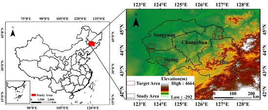
Figure 1.
Maps of the study area.
There are four distinct seasons in the study area, which has a temperate continental monsoon climate. It is located in China’s Northeast Plain, one of the three major black soil plains with good soil and high fertility, making the area suitable for crops. The main crop types that produce straw annually in the study area include maize, rice, and soybean. According to statistical data from 2020 yearbook of Jilin province, the total sown area for these three crops in the study area was 3,124,469, 490,231, 122,809 hectares, respectively. Jilin Province itself produced an annual straw output of more than 40 million tons [29]. The amount of crop straw produced is large, but in the study area, the overall utilization rate is significantly lower than the national average. In addition, the winters are cold, and the time window for returning straw to the fields is short. Therefore, straw is frequently discarded and burnt, which causes several environmental problems. Straw burning in this area usually occurs before spring plowing (April and May) and after the autumn harvest (October and November).
2.2. Data Sources
Sentinel-2 is a high-resolution multispectral imaging satellite constellation, including Sentinel-2A (launched in June 2015) and Sentinel-2B (launched in March 2017). One satellite has a 10-day revisit period, and together, they have a complementary 5-day revisit period. The Sentinel-2 satellites have a multispectral instrument (MSI) that can cover 13 spectral bands with spatial resolutions of 10, 20, or 60 m [30]. The Sentinel-2 satellite can provide high-resolution Earth observation data. The data have broad application prospects. Therefore, we used Sentinel-2 remote sensing images as the data source to construct a dataset of images showing smoke from straw burning.
In this study, we used Sentinel-2 image data captured under clear weather conditions. Interference from clouds and fog was excluded in advance. Information about the bands in the Sentinel-2 images is shown in Table 1. Sentinel-2 provides data at two processing levels: level 1C (L1C) and level 2A (L2A). L1C has undergone radiometric calibration and geometric correction, and L2A is the product of atmospheric correction based on L1C [31].

Table 1.
Waveband parameters of Sentinel-2.
There are many repositories of Sentinel-2 data, such as the United States Geological Survey, the European Space Agency (ESA), etc. This paper used Sentinel-2 data freely available on the ESA website (https://scihub.copernicus.eu/dhus/#/home, accessed on 27 April 2022). Since straw burning mainly occurs in April, May, October, and November, the imaging times were these months in 2021. The data level was L2A, and the latitude and longitude were from 121°38′ E to 131°19′ E and from 40°50′ N to 46°19′ N. We used four cloud-free and fog-free images with visible smoke to make datasets. The image information is shown in Table 2.
Table 2.
Images taken by Sentinel-2B under product grade MSIL2A.
2.3. Data Preprocessing
Sentinel-2 L2A data are radiometrically calibrated, geometrically corrected, and atmospherically corrected products. In this study, the spatial resolution of bands 2, 3, 4, and 8 is 10 m, and that of bands 11 and 12 is 20 m. To keep each band’s spatial resolution consistent, we used the nearest neighbor allocation method of the Sentinel Application Platform (SNAP) to resample all the bands to 10 m. The results were output in the IMG storage format, which is supported by The Environment for Visualizing Images (ENVI) [32]. Bands 4, 3, and 2 were synthesized using ENVI 5.3 to form Red-Green-Blue (RGB) images.
The four images have an average size of about 5000 pixels × 5000 pixels. From these images 893 sample images, we randomly cropped a size of 640 pixels × 640 pixels. Figure 2 shows examples of positive samples with smoke and negative samples without smoke. False positives were reduced using the negative samples.
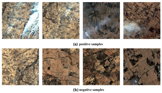
Figure 2.
Sample of (a) positive and (b) negative images.
2.4. Dataset Construction
After data pre-processing step, the smoke in all images was manually annotated. In order to increase the diversity of samples and avoid the overfitting problem of the model, data augmentation operations were performed on the marked images.
2.4.1. Data Labeling
The sample images were analyzed by visual interpretation using true-color synthesis (4-3-2), and then manually annotated. Visual interpretation has very high accuracy [33,34]. In Figure 3, the areas with smoke are marked with red boxes.
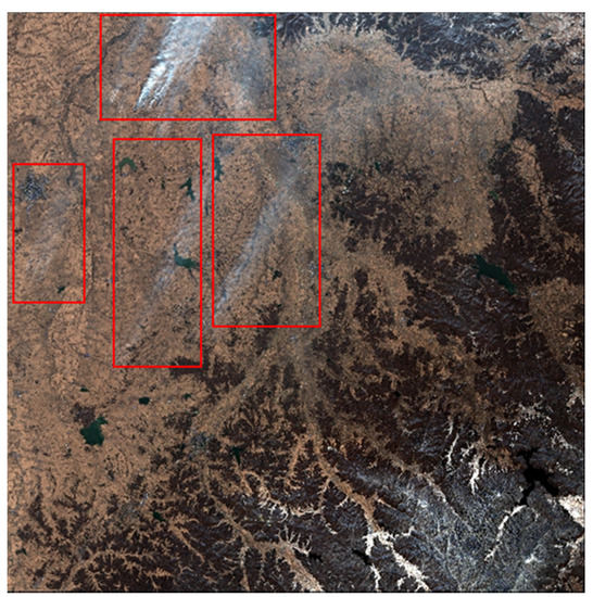
Figure 3.
The 4-3-2 band composite image.
In Figure 3, we can see the thin smoke produced by burning straw. During sampling, it was found that the 4-3-2 band composite images do not show the thin smoke clearly enough, so false color synthesis is necessary [34]. In this paper, for the synthesis, we considered one fire index (the modified normalized difference fire index (MNDFI)), two combustion indices (the burned area index (BAI) and the normalized burn ratio (NBR)), the normalized difference tillage index (NDTI), the modified crop residue cover (MCRC), and the normalized difference vegetation index (NDVI), as listed in Table 3.
Table 3.
Index descriptions and formulae.
B12 is the reflection value of the Band 12, B8 is the reflection value of the Band 8, B4 is the reflection value of the Band 4, B11 is the reflection value of the Band 11, and B3 is the reflection value of the Band 3.
Combining any three of the indices in Table 3, finally, the six best combinations based on the visual interpretation were selected and presented in Figure 4. The resulting synthetic images corresponding to Figure 3 are shown in Figure 4. The combination BAI-MCRC-MNDFI shows the thin smoke over land more clearly than the other combinations. Therefore, the analysis of the image samples in this paper was mainly based on the 4-3-2 band composite images, supplemented by images synthesized with the BAI-MCRC-MNDFI combination. Then, the images were labeled with boxes using the LabelImg tool. Since the base model uses YOLOv5s, all images were saved in YOLO format after the labeling was completed. For each image, the text file contained details such as the category of the sample and the label box dimensions (width and height of the label box, and center point coordinates).
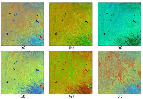
Figure 4.
Synthetic images for different combinations of index: (a) MNDFI-NDVI-NBR, (b) NDVI-MNDFI-BAI, (c) BAI-MCRC-MNDFI, (d) MNDFI-MCRC-NBR, (e) NDTI-MNDFI-BAI, and (f) MNDFI-NDTI-NBR.
2.4.2. Data Augmentation
The training of a deep learning model requires a large amount of data. To avoid the impact of model overfitting, an unbalanced data distribution, or using a single background on model training and testing, we augmented the data to expand the dataset. Operations included translations, rotations, mirroring, changing the brightness, adding noise, and cutting out. These operations were randomly applied to images with smoke, as shown in Figure 5.
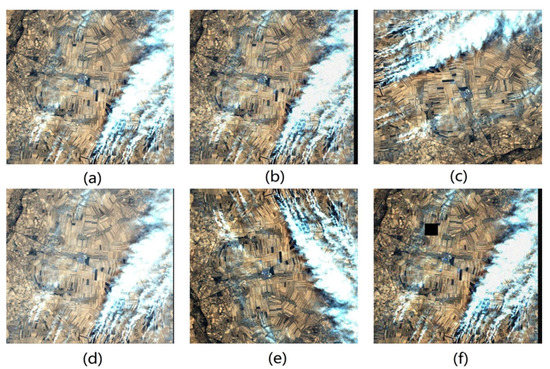
Figure 5.
Images of smoke from straw burning after various operations: (a) original image, (b) after translation + brightness + noise, (c) after rotation + brightness + flip, (d) after translation + brightness, (e) after brightness + flip, and (f) after translation + noise + cutout + brightness.
For the augmented images, to ensure the labels were consistent with the original image, any rotation, translation, or mirroring operations applied to an image were also applied to its labels [35].
Random rotation, translation, and mirror operations can enhance sample diversity and expand the amount of medium and small targets, which improve model recognition accuracy. Randomly changing the brightness of an image or adding noise can increase the stability of the model to a certain extent, even when it is disturbed. It can enhance the model’s robustness and reduce its sensitivity to the training data. For the cutout operation, a square area was randomly masked during training. This simple regularization technique can improve the robustness, generalizability, and performance for the model, and effectively avoid overfitting [36]. The dataset contained 4713 images after the above data augmentation.
The dataset was then divided into a training set, a validation set, and a test set in the ratio 6:2:2. These three sets had no regional overlaps. A model was constructed using the training and validation sets, while an evaluation of its accuracy was carried out using the test set.
2.5. YOLOv5s Model
As shown in Figure 6, YOLOV5s has four main components: input, backbone, neck, and prediction. The various modules are described below.
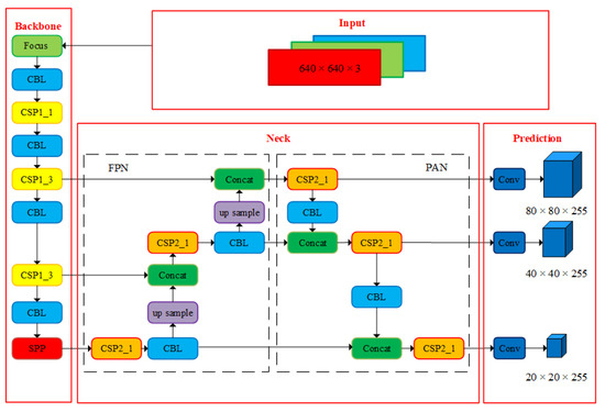
Figure 6.
YOLOv5s structure diagram.
2.5.1. Backbone Network
The backbone network of YOLOv5s has three main functional units: focus, spatial pyramid pooling (SPP) [37], and cross-stage partial connections (CSP) [38]. As shown in Figure 7, the slicing operation in the focus module converts the information in the wh plane to the channel dimension, and then extracts different features through convolution, which can reduce the information loss caused by down-sampling.
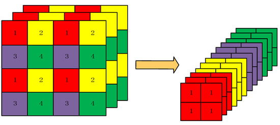
Figure 7.
Slice operation.
The input data is segmented into four slices [39], with a size of 3 × 2 × 2 per slice. Then, the concat operation is utilized to connect the four sections in depth, The size of output feature map being 12 × 2 × 2, which increases the dimensionality of the channel. This operation improves the receptive field of each point, reduces information loss, and improves the training speed.
The main function of the SPP module [37] is to fuse local and global features, which effectively broadens the range of the reception of backbone features and significantly separates the most crucial context features than simply using k × k maximum pooling.
CSP is a set of cross-stage residual units [38]. There are two CSP structures in YOLOv5s. One is used by the backbone network and has a residual unit, and the other is CSP2_X, which does not have a residual unit. CSP2_X is made by replacing the residual unit with ordinary CBL and applying it to the neck network, as shown in Figure 8. Compared with ordinary CBL, the CSP structure has significant advantages. It divides the feature into two branches and then uses the concatenation operation to better retain the feature information from different branches, which improves feature fusion.
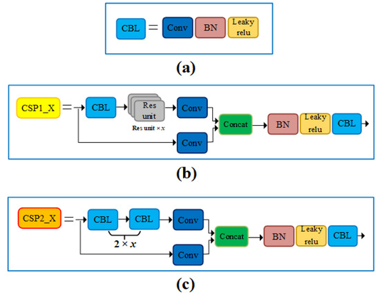
Figure 8.
(a) CBL structures, (b) CSP1_X structures, and (c) CSP1_X structures.
2.5.2. Neck Network
The neck module is a feature transfer network between the backbone network and the output layer. It samples and aggregates the eigenvalues extracted by the backbone network to form aggregated features at different scales. As shown in Figure 9, the neck network of YOLOv5s uses the feature pyramid network (FPN) [40] and the path aggregation network (PAN) [41]. FPN transfers and combines high-level feature information by up-sampling from the top to the bottom to convey strong semantic information. PAN is a bottom-up feature pyramid that conveys strong localization features. The simultaneous use of both can enhance the feature fusion and multi-scale prediction capabilities of different layers [42]. In the neck structure of YOLOv4, ordinary convolution operations are used [42]. In contrast, YOLOv5 uses the CSP2 structure, which was based on CSPNet, to enhance the network feature fusion.
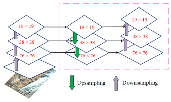
Figure 9.
FPN + PAN structure diagram.
2.6. Improved YOLOv5s Model
The original YOLOv5s is a 29-layer neural network built with structures such as Focus, CBL, CSP, and SPP. There are some smoke targets, however, that take up only a small area in the entire picture, which causes problems, such as missed and false detections. Thus, our paper adds an attention module after the backbone network and optimizes the activation function.
2.6.1. Optimizing the Backbone Network
The attention modules commonly used in object detection today are CBAM and the Squeeze-and-Excitation Network (SENet) [43]. Compared with SENet, CBAM has a spatial attention mechanism. In addition to considering the channel features of the target, it also focuses on the location information of the target [27]. In the remote sensing images obtained by satellites, there is low contrast between the target, the background, and complex scenes, Therefore, in order to enhance the feature expression ability of the model and enrich the information of smoke feature in the feature map, we introduced CBAM after the backbone network.
As shown in Figure 10, CBAM is structured as two independent modules, CAM and SAM. The input feature map is passed through CAM. Each channel undergoes both max pooling and average pooling. After a multi-layer perceptron, the resultant intermediate vector is added element-wise and sigmoid-activated to produce a channel attention [27]. is activated by to obtain the characteristic figure . The input to SAM is . This module performs average and maximum pooling in the channel dimension and obtains the spatial attention after a convolution operation and sigmoid activation. After is activated by , the final feature map is obtained:
where indicates element-wise multiplication.
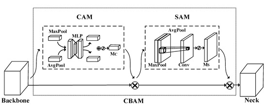
Figure 10.
Structure of CBAM. MLP, multi-layer perceptron.
The features at different scales are extracted by SPP, which is the last unit of the backbone network, and input into the CBAM module, which focuses on the channel features and location information, as these play a decisive role in the final prediction. CBAM emphasizes important smoke features and suppresses general features, which enhances the backbone network’s expression of features and improves the model’s prediction accuracy.
2.6.2. Improvement of the Nonlinear Activation Function
The smallest unit in the original YOLOv5s is the CBL structure, which is comprised of a convolutional layer, a batch normalization layer, and a nonlinear activation function. Nonlinear activation function is accountable for mapping the input and output of a neuron, and contributes significantly to learning the neural network model and understanding complex and nonlinear functions. The CBL structure of the original YOLOv5s uses the leaky ReLU activation function [44], which is a piecewise function. Since there are different interval functions, it is impossible to provide a consistent relationship in the prediction with positive and negative input values. This paper replaces the original activation function with the Mish function [28]:
The Mish function has no upper bound but has a lower bound, and it is a smooth and non-monotonic activation function [45]. Its derivative is:
where
Note:
The leaky ReLU and Mish activation functions and their derivatives are shown in Figure 11. The two functions are basically the same when x > 0. When x < 0, the Mish function is smoother than leaky ReLU. Therefore, the information can penetrate better into the neural network, thereby improving its accuracy and generalizability. Moreover, the Mish function is continuous, its derivative is continuous and smooth, and it can be differentiated everywhere. During backpropagation, it is easier to carry out gradient optimization with the Mish function, so that convergence is faster.
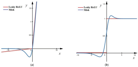
Figure 11.
(a) Activation function. (b) Derivative of the activation function.
2.7. Test Environment and Parameter Settings
All training and testing in this paper were performed on the same server, which had an Intel(R) Core (TM) i7-7820X Central Processing Unit (CPU), two 11 GB RTX 2080 Ti Graphic Processing Units (GPU), and 32 GB of running memory. We used Pytorch 1.5 as the deep learning framework. We wrote all of our programs in Python, and utilized the Compute Unified Device Architecture (CUDA) and Open-Source Computer Vision libraries (OpenCV). They all ran on Linux.
During training, 64 samples were used as a processing unit. The learning rate momentum was 0.937, the initial learning rate was 0.01, the weight decay was 0.0005, the optimization algorithm was SGD (stochastic gradient descent), and there were 600 iterations.
2.8. Evaluation Indicators
The value of the intersect over union (IOU) threshold is directly related to the output prediction frame. Generally, the larger the threshold, the higher the prediction accuracy [46]. The main evaluation indicators used in this paper are the mean average precision (mAP) for an IOU threshold of 0.5 (mAP50), mAP75, parameter size (MB), and the number of frames per second (FPS). mAP is an important metric for gauging detection accuracy of the target detection model. It is obtained from a precision (P)-recall (R) curve. The calculations for precision (P), recall (R), and mAP are as follows.
where the true positives (TP) are the number of positive images that are actually detected as being positive. FP refers to the number of false positives, which is the number of negative samples misclassified as positive samples. The false negatives (FN) are the number of positive samples that are wrongly detected as being negative. The quantity of detection target categories is K. K = 1 in this article. The average precision (AP) is the region enclosed by the coordinate axis and the P-R curve in a single-type detection, and mAP represents the average AP for every category.
3. Results
3.1. Comparison of Different Algorithms
The results for different algorithms in detecting smoke from straw burning are shown in Table 4. The Faster Region-Based Convolutional Neural Network (R-CNN) [47] and RetinaNet [48] did not do as well as the improved model for all four indicators (mAP75, mAP50, parameter size, and FPS). In terms of mAP75, Mask R-CNN [49] and Single-Shot Multibox Detector (SSD) [50] were better than the improved model, but not as good for mAP50, parameter size, and especially FPS. The detection speeds of Mask R-CNN and SSD were 1/20 and 1/10 that of the improved YOLOv5s model, respectively, which does not meet the requirements for efficient recognition. YOLOv5s outperformed the improved model in parameter size and FPS, but had a lower accuracy, since mAP75 and mAP50 were 3.67 and 1.15 percentage points lower than those for the improved YOLOv5s, respectively. When identifying smoke from straw burning, there is a high requirement for accuracy. Thus, the improved algorithm is better than YOLOv5s. Overall, the comparison of mAP75, mAP50, parameter size, and FPS shows that of the algorithms, the improved YOLOv5s model provides higher detection accuracy and faster speed.
Table 4.
Performance comparison of different smoke detection models.
3.2. Evaluation of the Improved Algorithm
Table 5 compares the experimental results for various versions of YOLOv5s. In YOLOv5s − Mish, leaky ReLU was replaced by the Mish activation function. YOLOv5s + CBAM is the original YOLOv5s with CBAM after the backbone network.
Table 5.
Performance comparison between different versions of YOLOv5s in detecting smoke.
The original YOLOv5s model had the fastest detection speed, but the lowest accuracy, as measured by mAP75 and precision. YOLOv5s − Mish, for which only the linear activation function has been optimized, has the same parameter size and detection speed as the original YOLOv5s model, but the precision, recall, and mAP75 were 1.03, 1.18, and 1.88 percentage points higher, respectively. Introducing only CBAM, the model parameters increased in size by 0.13 MB, the recall rate and detection speed decreased slightly, and the precision rate and mAP75 increased by 1.39 and 0.70 percentage points, respectively. The improved YOLOv5s method proposed in this paper combines the advantages of the two optimizations. Although the detection speed was slightly slower, the precision rate, recall rate, and mAP75 were better compared to the original YOLOv5s model by 1.71, 0.21, and 3.67 percentage points, respectively. Hence, this approach can realize the high precision and rapid identification of smoke from straw burning.
4. Discussion
4.1. Cloud and Haze
Smoke, clouds, and haze have very similar morphologies and spectral properties, so clouds and haze will affect the recognition results of smoke [51]. Moreover, with thick cloud cover, the information about smoke is completely lost. As a result, it is difficult to identify smoke accurately in satellite imagery [51].
To date, many scholars have performed extensive studies on de-clouding and dehazing of optical remote sensing images and have proposed several solutions. Using a wavelet transform, Li et al. [52] removed thin clouds from panchromatic remote sensing images. Markchom and Lipikorn [53] proposed a method for removing clouds using the HSI color space. Song et al. [54] created a method for cloud removal using single-scene remote sensing images. Li et al. [55] proposed a homomorphic filtering method for removing thin clouds. Although these traditional methods for removing clouds from optical remote sensing images have delivered satisfactory results, some of the methods for processing thin and thick clouds cannot be used universally, as they rely on prior knowledge. the feature information needs to be manually extracted, and the restored image details are inaccurate. Therefore, it is not feasible to use these traditional methods for cloud removal on a widespread basis.
With the development of machine learning, a support vector machine method was proposed by Liang et al. [56] that removes thick clouds and cloud shadows from remote sensing images. As compared to traditional methods, the method can better restore information about an object on the ground obscured by thick cloud. Deep learning has led to major breakthroughs in computer vision in recent years. In 2020, Pei et al. [51] provided a solution for removing clouds from optical remote sensing images used an improved conditional generative adversarial network (CGAN). A spatial pooling layer was introduced into the generator of the original CGAN, and regression loss was added, which improved the generation. In their experiments, this method achieved better results when removing cloud and in maintaining the fidelity of the images.
Due to the problems of low contrast and blurred details in foggy images, Yang et al. [57] decomposed an image into textural and structural layers, and dehazed the structural layers containing most of the fog. He et al. [58] provided an image dehazing method using the dark channel prior model, which is simple and effective but overestimates the density of the fog and distorts colors. With the development of deep learning, Cai et al. [59] used a convolutional neural network (CNN) to estimate the transmittance of haze. A model of atmospheric scattering was used to restore a haze-free image. Owing to its overreliance on atmospheric scattering, this indirect dehazing method can sometimes overestimate the transmittance despite achieving good results. The traditional method for dehazing an image relies on models of atmospheric scattering, which result in color distortions and insufficient dehazing. Using a residual attention mechanism, Yang et al. [60] proposed an end-to-end dehazing algorithm that effectively reduced the color distortion and the dehazing was less incomplete.
There are many other de-clouding and dehazing methods. Traditional and deep learning methods have their own advantages and disadvantages. Methods for removing cloud and fog from remote sensing images are very mature, and the image quality after cloud and fog removal is continually increasing. In the following research, we can refer to the abovementioned algorithms for de-clouding and de-hazing. In addition, we can utilize cloud and haze removal operations on the acquired remote sensing data in order to prevent clouds and haze from interfering with smoke detection and improve the model’s performance.
4.2. Other Artifacts
In addition to clouds and fog, there are other artifacts that can affect smoke identification, particularly weather attributes such as wind speed, direction, and humidity, which could impact the smoke formation and transport. In turn, this affects the accuracy of smoke identification models.
The data used in this study are Sentinel-2 remote sensing images under clear weather conditions. Smoke spreads more slowly in clear weather conditions and is easier to identify. Unlike previous studies, which have mostly focused on the pixel level [61], this study aimed to identify satellite images with smoke from straw combustion, that is, image-level smoke recognition. In pixel-level recognition, the location and type of target is estimated for each pixel in the image. Image-level smoke recognition learns the main features of smoke through training, and then identifies and locates the smoke with these features. This requires that, during training, the smoke features are as obvious as possible. Thus, we used 4-3-2 band composite images, as these can show smoke more clearly.
In order to enrich the characteristics of the smoke from straw burning as much as possible, reduce the influence of other artifacts on smoke recognition, and improve the accuracy of the model, in following research, we will use additional bands and indices in training. In addition to the indices in Table 3, 13 spectral bands of the Sentinel-2 Multispectral Imager (MSI) may be good candidates for the smoke recognition model. We can perform spectral analysis on different ground feature types (smoke vs. cloud, smoke vs. haze, smome vs. water, etc.), and select the bands and indices by the separability index (M) [62]. The separability index (M) is given by Equation (10):
where and are the mean and standard deviation of category i, respectively. The larger the value of M, the higher the separability between smoke and other ground objects; in other words, smoke is more accurately identified. The selected band and index were used as the model input, and the input combination with the best recognition effect was selected through ablation experiments.
Weather attributes will have a certain impact on the smoke detection model. For example, the smoke spreads quickly when the wind speed is high, and the smoke detection algorithm may not be able to detect the smoke in such circumstances. Therefore, we will explore the characteristics of smoke under different atmospheric diffusion conditions to find the maximum detection ability of the smoke detection algorithm.
5. Conclusions and Outlook
Detecting smoke is an important way to control straw incineration, which is an important for ensuring the ambient air quality and for sustainable agriculture. In this study, the YOLOv5s network model was used to detect smoke in remote sensing images. CBAM was added to YOLOv5s, and the Mish activation function was used instead of the leaky ReLU function. Our results indicated that the improved YOLOv5s maintained the original detection speed, with a detection speed of 476 frames per second, and achieved mAP75 and mAP50 values of 74.03% and 94.69%, respectively, which are 3.67 and 1.15% higher than those for the original algorithm. The improved model had both higher precision and recall rates than the original one. Therefore, the improved method proposed in this study can quickly and accurately identify smoke in the crop residue burning. This study may serve as a reference for improving the detection of smoke, and enhancing the effective management and control of straw burning.
In this study, the data only included cultivated land, and the smoke was entirely caused by straw burning. However, we found that the burning of biomass fuel, wood, coal, and other materials in the surrounding area also released smoke, which had a certain impact on the identification results of smoke produced by straw burning. In the future, we will identify the smoke shape through the model. Based on the shape of the smoke, factors such as wind speed, wind direction, and humidity will be taken into account to determine the source of the smoke. According to the source of the smoke, we can classify smoke into three categories: smoke from straw burning, smoke from domestic burning, and smoke from factories. Based on the characteristics analysis of different types of smoke, the ability of the model will be enhanced to distinguish smoke produced by straw burning.
Author Contributions
Conceptualization and design of the experiments, H.L., J.L. and J.D.; performed the experiments, H.L., B.Z. and W.Y.; data analysis and writing, H.L., Y.H. and D.L. All authors have read and agreed to the published version of the manuscript.
Funding
This research was funded as an environmental protection scientific research project of Jilin Provincial Department of Ecology and Environment, grant number E139S311; Jilin Province Development and Reform Commission, grant number 2020C037-7; and the Science and Technology Development Plan Project of Changchun, grant number 21ZGN26.
Institutional Review Board Statement
Not applicable.
Informed Consent Statement
Not applicable.
Data Availability Statement
The data that support the findings of this study are available from the corresponding author, [H.L.], upon reasonable request.
Acknowledgments
The authors would like to thank the ESA website for providing the Sentinel-2 data. All data and images in this paper were used with permission.
Conflicts of Interest
The authors declare no conflict of interest.
References
- Tipayarom, D.; Oanh, N.K. Effects from open rice straw burning emission on air quality in the Bangkok Metropolitan Region. Sci. Asia 2007, 33, 339–345. [Google Scholar] [CrossRef]
- The Beijing News. Available online: https://baijiahao.baidu.com/s?id=1664195319400703843&wfr=spider&for=pc (accessed on 6 March 2022). (In Chinese).
- Singh, G.; Gupta, M.K.; Chaurasiya, S.; Sharma, V.S.; Pimenov, D.Y. Rice straw burning: A review on its global prevalence and the sustainable alternatives for its effective mitigation. Environ. Sci. Pollut. Res. 2021, 28, 32125–32155. [Google Scholar] [CrossRef] [PubMed]
- Huo, Y.; Li, M.; Teng, Z.; Jiang, M. Analysis on effect of straw burning on air quality in Harbin. Environ. Pollut. Control 2018, 40, 1161–1166. (In Chinese) [Google Scholar]
- Ma, X.; Tang, Y.; Sun, Z.; Li, Z. Analysis on the Impacts of straw burning on air quality in Beijing-Tianjing-Hebei Region. Meteorol. Environ. Res. 2017, 8, 49. [Google Scholar]
- Kaskaoutis, D.G.; Kharol, S.K.; Sifakis, N.; Nastos, P.T.; Sharma, A.R.; Badarinath, K.V.S.; Kambezidis, H.D. Satellite monitoring of the biomass-burning aerosols during the wildfires of August 2007 in Greece: Climate implications. Atmos. Environ. 2011, 45, 716–726. [Google Scholar] [CrossRef]
- Wang, X. Grassroots environmental monitoring station to strengthen quality management research. Environ. Dev. 2017, 29, 162–163. (In Chinese) [Google Scholar]
- Rogan, J.; Chen, D. Remote sensing technology for mapping and monitoring land-cover and land-use change. Prog. Plan. 2004, 61, 301–325. [Google Scholar] [CrossRef]
- Wooster, M.J.; Roberts, G.J.; Giglio, L.; Roy, D.P.; Freeborn, P.H.; Boschetti, L.; Justice, C.; Ichoku, C.; Schroeder, W.; Davies, D.; et al. Satellite remote sensing of active fires: History and current status, applications and future requirements. Remote Sens. Environ. 2021, 267, 112694. [Google Scholar] [CrossRef]
- Chuvieco, E.; Aguado, I.; Salas, J.; García, M.; Yebra, M.; Oliva, P. Satellite remote sensing contributions to wildland fire science and management. Curr. For. Rep. 2020, 6, 81–96. [Google Scholar] [CrossRef]
- Simons, E.S.; Hinders, M.K. Automatic counting of birds in a bird deterrence field trial. Ecol. Evol. 2019, 9, 11878–11890. [Google Scholar] [CrossRef]
- Ma, L.; Wei, X.; Zheng, M.; Xu, P.; Tong, X. Research on straw burning detection algorithm based on FBF neural network. Comput. Netw. 2020, 24, 66–69. (In Chinese) [Google Scholar]
- Liu, X.; He, B.; Quan, X.; Yebra, M.; Qiu, S.; Yin, C.; Liao, Z.; Zhang, H. Near real-time extracting wildfire spread rate from Himawari-8 satellite data. Remote Sens. 2018, 10, 1654. [Google Scholar] [CrossRef] [Green Version]
- Xie, Y.; Qu, J.; Hao, X.; Xiong, J.; Che, N. Smoke Plume Detecting Using MODIS Measurements in Eastern United States. In Proceedings of the EastFIRE Conference Proceedings, Fairfax, VA, USA, 11–13 May 2005; pp. 11–13. [Google Scholar]
- Yamagishi, H.; Yamaguchi, J. Fire Flame Detection Algorithm Using a Color Camera. In Proceedings of the 1999 International Symposium on Micromechatronics and Human Science, Nagoya, Japan, 23–26 November 1999; pp. 255–260. [Google Scholar]
- Yamagishi, H.; Yamaguchi, J. A Contour Fluctuation Data Processing Method for Fire Flame Detection Using a Color Camera. In Proceedings of the 26th Annual Conference of the IEEE Industrial Electronics Society, Nagoya, Japan, 22–28 October 2000; Volume 2, pp. 824–829. [Google Scholar]
- Park, J.; Ko, B.; Nam, J.; Kwak, S. Wildfire Smoke Detection Using Spatiotemporal Bag-of-Features of Smoke. In Proceedings of the 2013 IEEE Workshop on Applications of Computer Vision, Clearwater Beach, FL, USA, 15–17 January 2013; pp. 200–205. [Google Scholar]
- Li, H.; Yuan, F. Image based smoke detection using pyramid texture and edge features. J. Image Graph. 2015, 20, 772–780. (In Chinese) [Google Scholar]
- Li, Z.; Khananian, A.; Fraser, R.H.; Cihlar, J. Automatic detection of fire smoke using artificial neural networks and threshold approaches applied to AVHRR imagery. IEEE Trans. Geosci. Remote Sens. 2001, 39, 1859–1870. [Google Scholar]
- Redmon, J.; Divvala, S.; Girshick, R.; Farhadi, A. You only Look once: Unified, Real-Time Object Detection. In Proceedings of the IEEE Conference on Computer Vision and Pattern Recognition, Las Vegas, NV, USA, 27–30 June 2016; pp. 779–788. [Google Scholar]
- Zhang, M. Insulator Detection and Defect Recognition in Transmission Line Patrol Image Based on Deep Learning. Master’s Dissertation, Xi’an University of Technology, Xi’an, China, 2021. [Google Scholar]
- Redmon, J.; Farhadi, A. YOLO9000: Better, Faster, Stronger. In Proceedings of the IEEE Conference on Computer Vision and Pattern Recognition, Honolulu, HI, USA, 21–26 July 2017; pp. 7263–7271. [Google Scholar]
- Mao, G.; Weng, W.; Zhu, J.; Zhang, Y.; Wu, F.; Mao, Y. Model for marine organism detection in shallow sea using the improved YOLO-V4 network. Trans. Chin. Soc. Agric. Eng. 2021, 37, 152–158. (In Chinese) [Google Scholar]
- Huang, L.; Wang, Y.; Xu, Q.; Liu, Q. Recognition of abnormally discolored trees caused by pine wilt disease using YOLO algorithm and UAV images. Trans. Chin. Soc. Agric. Eng. 2021, 37, 197–203. (In Chinese) [Google Scholar]
- Li, P.; Zhang, J.; Li, W. Smoke detection method based on optical flow improvement and YOLOv3. J. Zhejiang Univ. Technol. 2021, 49, 9–15. (In Chinese) [Google Scholar]
- Wu, D.; Lv, S.; Jiang, M.; Song, H. Using channel pruning-based YOLO v4 deep learning algorithm for the real-time and accurate detection of apple flowers in natural environments. Comput. Electron. Agric. 2020, 178, 105742. [Google Scholar] [CrossRef]
- Woo, S.; Park, J.; Lee, J.Y.; Kweon, I.S. CBAM: Convolutional Block Attention Module. In Proceedings of the European Conference on Computer Vision, Munich, Germany, 8–14 September 2018; pp. 3–19. [Google Scholar]
- Misra, D. Mish: A self regularized non-monotonic activation function. arXiv 2019, arXiv:1908.08681. [Google Scholar]
- Statistical Bureau of Jilin. Jilin Statistical Yearbook 2020; China Statistics Press: Beijing, China, 2020. [Google Scholar]
- Drusch, M.; Del Bello, U.; Carlier, S.; Colin, O.; Fernandez, V.; Gascon, F.; Hoersch, B.; Isola, C.; Laberinti, P.; Martimort, P. Sentinel-2: ESA’s optical high-resolution mission for GMES operational services. Remote Sens. Environ. 2012, 120, 25–36. [Google Scholar] [CrossRef]
- Louis, J.; Debaecker, V.; Pflug, B.; Main-Knorn, M.; Bieniarz, J.; Mueller-Wilm, U.; Gascon, F. Sentinel-2 Sen2Cor: L2A Processor for Users. In Proceedings of the Living Planet Symposium, Prague, Czech Republic, 9–13 May 2016; pp. 1–8. [Google Scholar]
- Johnson, A.D.; Handsaker, R.E.; Pulit, S.L.; Nizzari, M.M.; O’Donnell, C.J.; De Bakker, P.I. SNAP: A web-based tool for identification and annotation of proxy SNPs using HapMap. Bioinformatics 2008, 24, 2938–2939. [Google Scholar] [CrossRef] [Green Version]
- Tian, J.; Deng, R.; Qin, Y.; Liu, Y.; Liang, Y.; Liu, W. Visual Interpretation and Spatial Distribution of Water Pollution Source Based on Remote Sensing Inversion in Pearl River Delta. Econ. Geogr. 2018, 38, 172–178. [Google Scholar]
- Svatonova, H. Analysis of visual interpretation of satellite data. Int. Arch. Photogramm. Remote Sens. Spat. Inf. Sci. 2016, 41, 675–681. [Google Scholar] [CrossRef] [Green Version]
- Shao, H.; Ding, F.; Yang, J.; Zheng, Z. Remote sensing information extraction of black and odorous water based on deep learning. J. Yangtze River Sci. Res. Inst. 2021, 39, 156–162. (In Chinese) [Google Scholar]
- Yu, J.; Luo, S. Detection method of illegal building based on YOLOv5. Comput. Eng. Appl. 2021, 57, 236–244. (In Chinese) [Google Scholar]
- He, K.; Zhang, X.; Ren, S.; Sun, J. Spatial pyramid pooling in deep convolutional networks for visual recognition. IEEE Trans. Pattern Anal. Mach. Intell. 2015, 37, 1904–1916. [Google Scholar] [CrossRef] [Green Version]
- Wang, C.Y.; Liao, H.Y.M.; Wu, Y.H.; Chen, P.Y.; Hsieh, J.W.; Yeh, I.H. CSPNet: A New Backbone that Can Enhance Learning Capability of CNN. In Proceedings of the IEEE Conference on Computer Vision and Pattern Recognition, Seattle, WA, USA, 13–19 June 2020; pp. 390–391. [Google Scholar]
- Liu, T.; Zhou, B.; Zhao, Y.; Yan, S. Ship Detection Algorithm Based on Improved YOLOV5. In Proceedings of the International Conference on Automation, Control, and Robotics Engineering, Dalian, China, 15–17 July 2021; pp. 483–487. [Google Scholar]
- Lin, T.Y.; Dollár, P.; Girshick, R.; He, K.; Hariharan, B.; Belongie, S. Feature Pyramid Networks for Object Detection. In Proceedings of the IEEE Conference on Computer Vision and Pattern Recognition, Honolulu, HI, USA, 21–26 July 2017; pp. 2117–2125. [Google Scholar]
- Liu, S.; Qi, L.; Qin, H.; Shi, J.; Jia, J. Path Aggregation Network for Instance Segmentation. In Proceedings of the IEEE Conference on Computer Vision and Pattern Recognition, Salt Lake City, UT, USA, 18–22 June 2018; pp. 8759–8768. [Google Scholar]
- Bochkovskiy, A.; Wang, C.Y.; Liao, H.Y.M. Yolov4: Optimal speed and accuracy of object detection. arXiv 2020, arXiv:2004.10934. [Google Scholar]
- Hu, J.; Shen, L.; Sun, G. Squeeze-and-Excitation Networks. In Proceedings of the IEEE Conference on Computer Vision and Pattern Recognition, Salt Lake City, UT, USA, 18–22 June 2018; pp. 7132–7141. [Google Scholar]
- Maas, A.L.; Hannun, A.Y.; Ng, A.Y. Rectifier Nonlinearities Improve Neural Network Acoustic Models. In Proceedings of the International Conference on Machine Learning, Atlanta, GA, USA, 16–21 June 2013; Volume 30, p. 3. [Google Scholar]
- Yang, C.; Yang, Z.; Liao, S.; Hong, Z.; Nai, W. Triple-GAN with Variable Fractional Order Gradient Descent Method and Mish Activation Function. In Proceedings of the 12th International Conference on Intelligent Human-Machine Systems and Cybernetics, Hangzhou, China, 22–23 August 2020; Volume 1, pp. 244–247. [Google Scholar]
- Rahman, M.A.; Wang, Y. Optimizing Intersection-over-Union in Deep Neural Networks for Image Segmentation. In Proceedings of the International Symposium on Visual Computing, Las Vegas, NV, USA, 12–14 December 2016; Springer: Cham, Switzerland, 2016; pp. 234–244. [Google Scholar]
- Ren, S.; He, K.; Girshick, R.; Sun, J. Faster R-CNN: Towards real-time object detection with region proposal networks. Adv. Neural Inf. Process. Syst. 2015, 28, 2969239–2969250. [Google Scholar] [CrossRef] [Green Version]
- Lin, T.Y.; Goyal, P.; Girshick, R.; He, K.; Dollár, P. Focal Loss for Dense Object Detection. In Proceedings of the IEEE International Conference on Computer Vision, Venice, Italy, 22–29 October 2017; pp. 2980–2988. [Google Scholar]
- He, K.; Gkioxari, G.; Dollár, P.; Girshick, R. Mask R-CNN. In Proceedings of the IEEE International Conference on Computer Vision, Venice, Italy, 22–29 October 2017; pp. 2961–2969. [Google Scholar]
- Liu, W.; Anguelov, D.; Erhan, D.; Szegedy, C.; Reed, S.; Fu, C.Y.; Berg, A.C. SSD: Single Shot Multibox Detector. In Proceedings of the European Conference on Computer Vision, Amsterdam, The Netherlands, 11–14 October 2016; pp. 21–37. [Google Scholar]
- Pei, A.; Chen, G.; Li, H.; Wang, B. Method for cloud removal of optical remote sensing images using improved CGAN network. Trans. Chin. Soc. Agric. Eng. 2020, 36, 194–202. (In Chinese) [Google Scholar]
- Li, C.; Deng, X.; Zhao, H. Thin cloud removal algorithm based on wavelet analysis for remote sensing images. Digit. Technol. Appl. 2017, 6, 137–139, 143. (In Chinese) [Google Scholar]
- Markchom, T.; Lipikorn, R. Thin cloud removal using local minimization and logarithm image transformation in HSI color space. In Proceedings of the 2018 4th International Conference on Frontiers of Signal Processing (ICFSP), Poitiers, France, 24–27 September 2018; pp. 100–104. [Google Scholar]
- Song, X.; Liu, L.; Li, C.; Wang, J.; Zhao, C. Cloud removing based on single remote sensing image. Opt. Technol. 2006, 2, 299–303. (In Chinese) [Google Scholar]
- Li, H.; Shen, H.; Du, B.; Wu, K. A High-fidelity method of removing thin cloud from remote sensing digital images based on homomorphic filtering. Remote Sens. Inf. 2011, 30, 41–44, 58. (In Chinese) [Google Scholar]
- Liang, D.; Kong, J.; Hu, G.; Huang, L. The removal of thick cloud and cloud shadow of remote sensing image based on support vector machine. Acta Geod. Cartogr. Sin. 2012, 41, 225–231, 238. (In Chinese) [Google Scholar]
- Yang, A.P.; Xing, J.N.; Liu, J.; Li, X.X. Single image dehazing based on middle channel compensation. J. Northeast. Univ. 2021, 42, 180–188. [Google Scholar]
- He, K.; Sun, J.; Tang, X. Single image haze removal using dark channel prior. IEEE Trans. Pattern Anal. Mach. Intell. 2010, 33, 2341–2353. [Google Scholar]
- Cai, B.; Xu, X.; Jia, K.; Qing, C.; Tao, D. Dehazenet: An end-to-end system for single image haze removal. IEEE Trans. Image Process. 2016, 25, 5187–5198. [Google Scholar] [CrossRef] [Green Version]
- Yang, Z.; Shang, J.; Zhang, Z.; Zhang, Y.; Liu, S. A new end-to-end image dehazing algorithm based on residual attention mechanism. J. Northwest. Polytech. Univ. 2021, 39, 901–908. [Google Scholar] [CrossRef]
- Karimi, H.; Navid, H.; Seyedarabi, H.; Jørgensen, R.N. Development of pixel-wise U-Net model to assess performance of cereal sowing. Biosyst. Eng. 2021, 208, 260–271. [Google Scholar] [CrossRef]
- Giglio, L.; Loboda, T.; Roy, D.P.; Quayle, B.; Justice, C.O. An active-fire based burned area mapping algorithm for the MODIS sensor. Remote Sens. Environ. 2009, 113, 408–420. [Google Scholar] [CrossRef]
Publisher’s Note: MDPI stays neutral with regard to jurisdictional claims in published maps and institutional affiliations. |
© 2022 by the authors. Licensee MDPI, Basel, Switzerland. This article is an open access article distributed under the terms and conditions of the Creative Commons Attribution (CC BY) license (https://creativecommons.org/licenses/by/4.0/).