The March 2012 Heat Wave in Northeast America as a Possible Effect of Strong Solar Activity and Unusual Space Plasma Interactions

Abstract

In the past two decades, the world has experienced an unprecedented number of extreme weather events, some causing major human suffering and economic damage. The March 2012 heat wave is one of the most known and broadly discussed events in the Northeast United States (NE-USA). The present study examines in depth the possible influence of solar activity on the historic March 2012 heat wave based on a comparison of solar/space and meteorological data. Our research suggests that the historic March 2012 heat wave (M2012HW) and the March 1910 heat wave (M1910HW), which occurred a century earlier in NE-USA, were related to Sun-generated special space plasma structures triggering large magnetic storms. Furthermore, the largest (Dst = −222 nT) magnetic storm during solar cycle 24 in March 2015 (only three years later than the March 2012 events) occurred in relation to another heat wave (M2015HW) in NE-USA. Both these heat waves, M2012HW and M2015HW, resemble each other in many ways: they were characterized by extremely huge temperature increases ΔΤ_Μ = 30° and 32° (with maximum temperatures Τ_Μ = 28° and 23°, respectively) during a positive North Atlantic Oscillation index, the high temperatures coincided with large-scale warm air streaming from southern latitudes, they were accompanied by superstorms caused by unexpected geoeffective interplanetary coronal mass ejections (ICMEs), and the ICME-related solar energetic particle (SEP) events were characterized by a proton spectrum extending to very high (>0.5 GeV) energies. We infer that (i) all three heat waves examined (M2012HW, M2015HW, M1910HW) were related with strong magnetic storms triggered by effective solar wind plasma structures, and (b) the heat wave in March 2012 and the related solar activity was not an accidental coincidence; that is, the M2012HW was most probably affected by solar activity. Future case and statistical studies are needed to further check the hypothesis put forward here, which might improve atmospheric models in helping people’s safety, health and life.

1. Introduction

A Contemporary Scientific and Social Problem: Τhe Challenge of Extreme Weather Events

In [1], we studied a barrage of intense space weather phenomena in March 2012 including one of the largest geomagnetic storms of solar cycle 24. March 2012 was also reported as a period with global extreme weather events, with the well known being the “historic heat wave” in North America. The “historic heat wave” in North America was broadly discussed in scientific website reports, such as in NASA and NOAA scientific papers [2,3,4,5], and newspapers (New York Times, The Guardian, etc). Refs. [6,7,8] provided observations in the upper and lower atmosphere, and they pointed out the time coincidence with the unusual solar activity. Scott [6] noted that “The heat wave that affected the eastern and central United States in March 2012 coincided with a flurry of solar eruptions, and it’s not unreasonable to wonder if such events are related. After all, the Sun’s energy is the source of Earth’s warmth”.

Indeed, the Sun is the major energy source of our planet, and its electromagnetic activity influences in many ways the planet itself and its environment (lithosphere, atmosphere, biosphere, technosphere, ozonosphere, ionosphere, magnetosphere). Furthermore, it has been noted that “Solar terrestrial exploration can help establish the physical cause and effect relationships between solar stimuli and terrestrial responses. When these relationships are understood, science will have an essential role for weather and climate prediction.” This statement was part of an early proposal by R. D. Chapman submitted to NASA [9]. This statement has gained new interest nowadays, since new significant information has come to light on the influence of solar activity on weather variations, and on the other hand, we have seen an unprecedented number of extreme weather events in the last decades, some causing significant human suffering and economic damage [10].

For instance, more than 70,000 additional deaths occurred in Europe during the summer of 2003. In the years 2010–2011, unprecedented numbers of extreme weather events occurred across the globe. The Center for Climate and Energy Solutions (CCES) also noted that the 12-month period from September 2010 to August 2011 was the driest on record in Texas with total direct losses to crops, livestock, and timber estimated at more than $10 billion (https://www.c2es.org/2011/12/extreme-weather-in-2011/, accessed on 27 May 2022).

Recently, extreme heat and wildfires occurred in southern Europe at the beginning of August 2021, with a heat wave in Greece reaching a maximum temperature of 47.1 degrees Celsius. In July 2021, heavy rain caused chaos in parts of Germany and neighboring countries, with many people dead and many missing. Munich estimates that natural disasters caused more than $90 billion global direct losses in 2015 (Attribution of Extreme Weather Events in the Context of Climate Change, National Academies of Sciences, Engineering, and Medicine Report. Washington, DC: The National Academies Press. 21–24. doi:10.17226/21852). The great number of unpredictable physical catastrophes suggests that a multidisciplinary approach to extreme weather events may increase their predictability.

Major changes in solar activity in the past centuries causing significant influences in Earth’s climate are broadly known in the scientific community as the historic Maunder minimum (MM), between AD 1650 and 1715 [11] and Medieval warm period, around the year 1000 AD [12]. Nowadays, of particular interest is the question of whether extreme solar events may cause extreme weather events [7,8] and, if so, whether we can predict them by incorporating space weather prediction results in atmospheric model.

The scope of the present work is to address the above question by examining the possible dependence of extreme weather events on unusual solar conditions. To this end, we investigate, for the first time, the possible space influence on near-ground air temperature by comparing simultaneous space and terrestrial observations during March 2012 and March 2015 magnetic superstorms. More specifically, we present and analyze as case studies the March 2012 and March 2015 magnetic superstorms with March 2012 heat wave events and the comparable temperature increase during the highest magnetic storm of solar cycle 24 in March 2015. Meteorological time series are used for the near-ground weather in Madison, Wisconsin. In particular, the M2012HW is compared with a previous greatly important March heat wave in the Northeast United States (NE-USA) in 1910.

The main result of the present study is that ICME-related Solar Energetic Particle (SEP) events with proton spectrum extending to very high (>0.5 GeV) energies and reaching Earth’s environment, under some unusual interplanetary conditions, seem to play a major role in the March 2012 heat wave event in NE-USA (Madison, Wisconsin). This finding is consistent with a large series of studies suggesting a solar influence on Earth’s lower atmosphere, but it extends, for the first time, previous results at low altitudes (≈2000 km) to near-ground data.

2. Solar–Atmospheric Weather Relationships

2.1. Extreme Weather Events: Anthropogenic versus Physical Agents

Global warming has been considered to be the agent of frequent heat waves and other extreme phenomena in the last few decades [10,13]. According to [14], scientists have published more than 350 peer-reviewed studies looking at weather extremes around the world, from heat waves in Sweden [15] and droughts in South Africa [16] to flooding in Bangladesh [17] and hurricanes in the Caribbean [18]. Ref. [14] concludes that the results provide mounting evidence that human activity is raising the risk of some types of extreme weather, especially those linked to heat. Furthermore, many authors claim that this statement does not mean that climate change can be blamed for every extreme weather or climate event. Some extreme events have been explained in terms of natural variations [19,20,21].

Ref. [14] claim that scientists found no discernible influence owing to human activity in 10% of extreme weather events and trends studied. For a further 11%, the observational data or modeling techniques used in the study were insufficient to reach a reliable conclusion. Of the 132 attribution studies that have looked at extreme heat worldwide, 122 (92%) found that climate change had made such an event more likely or more severe. External forcing may play a role that could be crucial for specific cases, and long-term climate changes may influence the probability and the magnitude of extreme weather events [22]. A review paper by [23] reached the conclusion that the debate on “anthropogenic versus solar influence” has not yet been satisfactorily answered, and further analysis and discussion is needed.

The Sun is the ultimate energy source of the terrestrial climate, vegetation, and life, while, apart from electromagnetic radiation, it affects the atmospheric weather via SEP events and probably other solar wind interaction processes (see Section 2.3). Therefore, it is reasonable to examine whether solar activity effects may contribute to a class of extreme atmospheric changes in the near-ground troposphere [6,7,8,23,24].

Although much is known about solar/space agents of tropospheric variations, such as UV variations and SEP events, the causal mechanisms for the possible short-term solar space- near-ground air temperature effects remain obscure. Refs. [7,8] have shown in preliminary results that the historic March 2012 heat wave in NE-USA and the associated global weather anomalies occurred during a CME-related SEP event and a subsequent magnetic storm. The present paper further elaborates the long chain of solar–interplanetary space–magnetospheric–atmospheric physical features for this special period (in comparison with heat waves in March 1910 and March 2015).

2.2. Violent Sun and Disturbed Interplanetary Space

Energetic particles (protons and electrons) accelerating during solar flares (SFs) can reach Earth in less than 0.5 h. The coronal mass ejections (CMEs) often related with SF occurrence are also closely associated with solar energetic particles (SEP), which reach the Earth’s orbit in a time period ranging from ≈15 h to a few days [25,26,27]. Therefore, an SEP event observed by a satellite near Earth may be composed of both: (a) energetic particles that run from the Sun at high speeds along the IMF lines and (b) energetic particles reaching later, which have been accelerated and controlled by the ICME and the associated IP shock wave. A magnetohydrodynamic shock can accelerate particles via two processes: (1) diffusive shock acceleration, which is a Fermi 1 acceleration process [28,29] or (2) the shock drift acceleration, which is also called scatter-free shock acceleration [30,31].

Figure 1 displays the flux-time profile of energetic (1880–4700 keV) protons of the main SEP event associated with two SFs on 7 March 2012 and an integrated SEP event (thereafter: SEPI) from 4 to ≈20 March composed of successive individual SEP events. This SEP event will be further examined in the next sections in relation with the March 2012 heat wave, but it is used here as an example to describe the main features of an SEP event as observed in the near-Earth IP space.

The SEP onset may be due to particles accelerated at the Sun, such as the flux increase marked as Phase I in Figure 1. The SEP onset is often followed by an energetic particle structure with a more or less gradual flux enhancement (Phase II, Figure 1), which is centered at the IP shock (Phase III, Figure 1) and is composed of particles accelerated at the traveling shock front or its vicinity. After the shock-related peak, the flux decreases gradually (Phase IV, Figure 1), as long as the IP shock leaves the near-Earth detecting satellite.

The SEP events actually show a variety of features concerning time profile, time duration, particle composition, and energy spectrum. The type of CME impact on Earth’s magnetosphere depends on various solar and interplanetary conditions. Definitely, its source site on the Sun plays an important role in the flux-time profile observed near-Earth [25,32].

We also refer to two main types of flux-time profiles, the gradual or CME-related events and the impulsive or flare-related events. The gradual or CME-related events typically last several days, as in the 7–9 March 2012 event shown in Figure 1, while the impulsive or flare-related events last a few hours. Impulsive events are typically observed when the observer is well magnetically connected to the flare site [33].

The SEP energy spectrum extends up to several GeV. Several tens of MeV protons must be accelerated early in the impulsive phase, while the injection of some ten or hundred MeV proton energies occurs significantly later [34]. Very high energy solar particles are observed either by satellites or ground-based experiments such as neutron monitors (NMs). The SEP events observed by NMs are called ground-level enhancements or simply GLEs. ΝΜs measure secondary particles that are produced when ions with energies above several hundred of MeVs create a nuclear cascade in the Earth’s atmosphere [35,36].

Kühl et al. [37] identified only 42 SOHO SEP events with energies >500 MeV during a period of ≈20 years (1995–2015), which suggests an average frequency as low as ≈2 events/year. This result suggests that SEP events with an energy spectrum extending to energies >500 MeV occur rarely in Earth’s orbit, and this is the case of the March 2012 SEP event we examine in the present paper in relation to the March 2012 heat wave.

2.3. Solar Particle Radiation and Atmospheric Weather Relationships

2.3.1. Solar Energetic Particles

In the last decades, the research on solar–tropospheric relationships has emphasized long-time (i.e., solar cycle) climate trends of stratospheric changes, and polar temperatures, cloudy, winds, and sea and surface temperatures [38]. Today, there is strong evidence for solar cycle (≈11-year periodicity) influence on stratospheric changes, polar temperatures, winds, global cloudy, north Atlantic oscillation, and some more environmental phenomena [38,39].

However, various studies of meteorological responses to short-term transient events on the Sun have also gathered significant information. Thus, it is now broadly accepted that solar activity affects both the atmospheric climate and weather [23,24,38,40,41,42,43,44,45].

We have already mentioned that CMEs are known to drive IP shock waves with an average speed of ≈350–470 km/sec and with extreme values reaching Vsw > 2000 km/sec [27,46]. These speeds correspond to a time delay between the CME generation on the Sun and the subsequent effect (magnetic storm, etc.) on Earth in a range between ≈5 days to less than 1 day, which is the expected time delay for an SF/CME influence on atmospheric weather. We point out that the ICME reaches Earth later (number of days) than the high-speed SEPs, which reach the Earth directly (within a few hours or even <1 h) following the IP field lines, after their generation on the Sun.

Meteorological responses to short-term transient events on the Sun have been reported from the beginning of the space era. For instance, Schuurmans et al. [47] examined the average change in the height of several constant pressure levels in the troposphere and lower stratosphere after intense SFs in the northern hemisphere (≥10° N). They found statistically significant features of the reaction pattern at high as well as at low latitudes. Their results identified changes in the properties of the reaction pattern within 6 h after the flare, with the maximum response occurring near the tropopause. They suggested that the atmospheric reaction pattern can be attributed to SEP events observed by satellites rather than enhanced ultraviolet radiation. Schuurmans [40] reported that tropospheric effects were found to occur at 2–4 days after a solar flare, which is consistent with the arrival time of ICMEs, which are released from the Sun.

A significant maximum of cosmogenic 7Be and 32P concentrations in the air was found in Bavarian Alps (Zugspitze peak, ≈3 km above sea level), which are by far preponderantly generated in the lower stratosphere. The concentration maxima observed about 2–3 days after the flare event were found to coincide in time with maxima of solar wind velocity and geomagnetic index Ap. This time delay also corresponds to the travel time of CMEs and the arrival at Earth of the ICME-related SEP events, which is in agreement with the results of [40].

Pudovkin and Raspopov [48] and Pudovkin and Babushkina [49] further confirmed that solar activity can directly affect the lower atmosphere by changing its thermal state. Furthermore, a study of ≈10-year data of satellite observations (NIMBUS 7, SMM, etc.) of the total solar irradiance (TSI) indicated that the solar irradiance changed only slightly (≈0.1% of the mean TSI) during the 11-year solar cycle [50], which suggests that solar and galactic cosmic rays could be the main agent transferring the solar activity influence to the lower atmosphere.

Avakyan et al. [43] studied the meteorological variations at low height during one of the major and well-known solar events of the last decades: the Halloween October 2003 solar events. In particular, they studied the air temperature T and the atmospheric pressure P during the extreme events of October 2003 at the mountain meteorological observatory near Kislovodsk (2100 m above sea level); they observed a T increase after large magnetic storms (Kp > 5) in 16 (84% of) cases, and they claimed that the manifestation of solar flares and magnetic storms in weather parameters, such as temperature, at an altitude of 2100 m was proven. In addition, strong electric field fluctuations were reported after the great Halloween events (28 and 30 October 2013) in Kamchatka, while many other researchers also reported various other atmospheric reflections following the October 2003 solar events [51,52].

We infer that several tropospheric effects were confirmed by several investigators to occur at 2–4 days after a flare/CME on the Sun. This time delay is consistent with the CME propagation time from the Sun to the Earth and strongly suggests a tropospheric response to ICMEs reaching the Earth’s atmosphere.

Furthermore, besides solar cosmic rays, galactic cosmic rays appear to play a significant part in climate and weather [53,54,55,56,57].

Although the large-scale anthropogenic influences on the Earth’s environment in the 20th–21st centuries are blamed for the frequent occurrence of extreme weather events, the fact that such events occurred in the past centuries suggests that it is not impossible for them to occur nowadays as well. Moreover, the confirmed SEP-tropospheric effects and the frequent occurrence of extreme weather events in the last decades pose new reasonable questions: (1) Can we find any direct observational evidence that solar activity driving terrestrial effects may also trigger extreme tropospheric extremes revealed by near-ground atmospheric parameters (temperature, wind, electric field)? (2) If so, under which space and/or terrestrial conditions? These questions are seriously addressed for the first time in the next sections.

2.3.2. Solar and Geomagnetic Activity

ΙCME-driven storms, associated with SEPs, produce various electromagnetic phenomena in the Earth’s environment. The magnetic storms accelerate particles at various sites of the Earth’s environment ([1,58,59,60] and references therein). A large amount of the energetic particles are accelerated in the plasma sheet and in the radiation belts and precipitate into the ionosphere and the upper atmosphere following geomagnetic field lines [61,62,63], while other particles escape from the magnetosphere into the magnetosheath and, from therein, into the interplanetary space [64,65,66,67]. Therefore, it is expected that such magnetospheric particles would be observed outside the Earth’s bow shock after the incidence of the ICME on the Earth’s magnetosphere in March 2012.

Sepalla et al. [68] claimed that solar activity controlled magnetospheric electron and proton precipitation in the atmosphere produces a potential influence on stratospheric circulation. Moreover, they suggested that magnetospheric particle precipitation forcing the atmosphere is as intense as that arising from the solar irradiance variations.

Kleimonova et al. [69] examined variations in the vertical atmospheric electric field component Ez in the absence of local geomagnetic disturbances. They reported considerable (≈100–300 V/m) decreases in the electric field component Ez at Swider midlatitude Poland observatory (geomagnetic latitude 47.8°), under the conditions of fair weather, which were observed simultaneously with the substorm onset in the nighttime sector of auroral latitudes (College observatory). They inferred that an intensification of the IP electric field during the magnetic storm main phase, the development of magnetospheric substorms and the precipitation of energetic electrons into the nighttime auroral ionosphere can result in considerable disturbances in the midlatitude atmospheric electric field.

In a recent review, Michnowski et al. [70] reported that the simultaneous detection of solar wind parameters, magnetic storms and variations of the DC vertical atmospheric electric field Ez and current density, Jz, measured at ground level in the Arctic, at the S. Siedlecki Polish Polar Station Hornsund, Spitsbergen (Svalbard, Norway), and at the mid-latitude S. Kalinowski Geophysical Observatory in Swider (Poland) confirms their relationship. They infer that their observations allow the conclusion that the physical dependence of ground-level Ez and Jz on solar wind changes produce measurable effects, and they expect that it would be more evident at middle latitude during strongly disturbed circumstances, following solar flares and the Earth-directed CMEs.

2.4. March 2012 Temperature Anomaly in Northeast America

The March 2012 global extreme weather events, and in particular, the “historic heat wave” in North America at those times, is an example of an extreme weather event that was attributed to a natural and not a greenhouse gases (GHG) effect. The question that several scientists addressed is the following: could the March 2012 heatwave have been anticipated?

A relative report on the so-called “Meteorological March Madness 2012” by the NOAA Physical Sciences laboratory discusses the March 2012 as follows: “It fails to anticipate the specific location of the 2012 heatwave over the Upper Midwest/Ohio Valley region since the magnitude of the greenhouse gases (GHG) signal is not materially different for the western U.S., central U.S., and eastern U.S., or for that matter for Alaska, and Asia which, during this period, experienced severe cold. And, the GHG warming signal fails to explain the extreme magnitude of the heat wave event, which achieved daily departures of +20 °C, or about 20-fold greater than the estimated background warming signal. Our physically based analysis explored the possibility for strong nonlinear amplifying feedbacks or highly nonlinear dynamical sensitivity to GHG forcing, and these models which represent such process in their integration of the coupled climate system, are consistent with that empirical assessment that such processes were unlikely of primary significance over the U.S. during March 2012” [71]. In Chicago, the National Weather Service described the heat wave as “historic and unprecedented” (https://www.weather.gov/lot/march2012_heat accessed on 27 May 2022). Dole et al. [3] noted that “The numbers were stunning” concerning the March anomaly and that “Nature’s exuberant smashing of high temperature records in March 2012 can only be described as “Meteorological March Madness”.

The March 2012 heat wave was also called a “black swan event” (https://psl.noaa.gov/csi/events/2012/marchheatwave/anticipation.html (accessed on 23 May 2022).

Borth et al. [2] and Dole et al. [3] reached the conclusion that the superposition of a strong natural variation together with a long-term regional warming of approximately 1 °C would be sufficient to account for the extreme magnitude of the March 2012 temperature anomalies. This suggests that a nonlinear response to climate change is not required to explain either the occurrence or exceptional magnitude of this event. These studies suggest that a combination of atmospheric conditions can explain the daily mean temperatures which reached values of 15–20 °C or more above normal during the peak of the event.

As we have mentioned, the purpose of the present study is to examine whether the elaboration of the coincidence of the solar activity with the March 2012 heat wave might support their physical link. For this reason, in the next section, we briefly report the instrumentation and the kind of space and terrestrial data we used. In Section 3, we show the results from the comparative analysis of simultaneously obtained space and terrestrial measurements during the March 2012, March 2015 and March 1910 heat waves in NE-USA. In Section 4, we check the hypothesis of the possible physical links between space and near-ground atmospheric weather in March 2012 in NE-USA in comparison with two other similar events: March 2015 and March 1910 extreme space weather and corresponding heat waves. In Section 5, we discuss the possibility of the solar influence on the March 2012 heat based on the comparison of observations on March 1910, March 2012 and March 2015 heat waves. Finally, in Section 6, we summarize the results of the extreme all three weather events in March 2012, March 2015 and March 1910, in the framework of Sun–Earth relationships and make some conclusions and suggestions for further research on the possible Sun–extreme weather relationships.

3. Data

In this study, we use for the first time simultaneously obtained solar, space and terrestrial measurements in order to investigate, also for the first time, the possible correlation between extreme solar/space activity with a well-known extreme weather event on the Earth. For this reason, we directly compare time series of energetic particle flux in space, of the index Dst of geomagnetic activity, and the near Earth’s ground meteorological parameters. We also examine the North Atlantic Oscillation (NAO) index.

The energetic proton and electron analysis in the IP space is based on measurements obtained by the NASA Advanced Composition Explorer (ACE) satellite [72]. ACE is a spacecraft (http://www.srl.caltech.edu/ACE/, accessed on 27 May 2022), circulating the L1 Lagrangian point (Figure 2a), where L1 is the point of Sun–Earth gravitational equilibrium, at a distance of ≈220 R_E from the Earth (Figure 2b; R_E is the length of the Earth’s radius). ACE was launched on 25 August 1997 from the Kennedy Space Center in Florida and has been continuously providing in situ observations up to the present day (https://www.swpc.noaa.gov/products/ace-real-time-solar-wind, accessed on 27 May 2022).

Solar activity and geomagnetic storms are related with ionospheric and atmospheric changes. When reporting space weather, ACE provides an advance (≈1 h) warning of geomagnetic storms. Real-time observations with 1 s resolution are provided continuously to the Space Environmental Center (SEC) of the National Oceanographic and Atmospheric Association (NOAA). Space weather prediction is a space research direction of high importance to understand and predict a variety of phenomena at the Earth and its close environment: if the results of our present study are further confirmed, we believe that such measurements could be useful to improve predictions of extreme atmospheric events.

For the needs of our study, we used data from the EPAM (Electron, Proton, and Alpha Monitor) particle instrument (http://sd-www.jhuapl.edu/ACE/EPAM, accessed on 21 May 2015; http://www.srl.caltech.edu/ACE/ASC/level2/lvl2DATA EPAM.html, accessed on 21 May 2015). In particular, we analyzed measurements from the channels P2’ (ions), DE1 (electrons) and P8 (ions) from the LEMS120, LEFS150, and LEMS30/EPAM telescopes. The numbers of these telescopes designate the angular orientation in degrees (1500, 1200, and 300) from the center of each channel with respect to the spacecraft spin axis, which is always pointed toward the Sun [73]. Therefore, it is evident that P8 ions and P2’ ions/DE1 electrons and ions meet the LEMS30 and LEMS120/LEFS150 telescopes from the general Sunward and anti-Sunward direction. The telescope direction helps us to understand the solar or terrestrial (magnetospheric) origin of the energetic particles upstream from the Earth’s bow shock. Since most of the ions measured are protons, we call the ion measurements “proton” measurements. Therefore, the P8/LEMS30 protons are mostly of solar origin, whereas the P2’ protons/DE1 electrons are of magnetospheric origin.

The three EPAM/ACE channels we chose, namely P’2, P8, and DE1, measure low energy (≈70–115 keV) protons, relatively high energy (1880–4700 keV) protons, and low energy (≈40–50 keV) electrons, respectively. These three channels, P’2, P8, and DE1, were selected in order to distinguish between particles originated from two sources: the Sun and the magnetosphere. In addition, we note that the long time (several days) high-energy proton structures observed by the P8 channel are indicative of a solar origin. The short time (several seconds to few hours) events of low-energy protons and electrons from P’2 and DE1 channels in the vicinity of the Earth, record particles leaking from the Earth’s magnetosphere [67,73,74]. Thus, identifying the different types of energetic charged particles in the region upstream from the Earth’s bow shock (the boundary of the Earth’s magnetosphere) allows us to focus on the possible relation between solar energetic particle events and atmospheric weather variations or magnetospheric particle events and atmospheric weather variations.

The status of the magnetosphere was based on measurements from the World Data Center for Geomagnetism, Kyoto (http://wdc.kugi.kyoto-u.ac.jp/dstdir/, accessed on 15 May 2015) and in particular on the values of the Dst index, for the data analysis of March 2012 and 2015 events. Dst is an index of magnetic activity derived from a network of near-equatorial geomagnetic observatories that measures the intensity of the ring current, which is a globally symmetrical equatorial electrojet. The index Dst is derived from hourly scalings of low-latitude horizontal magnetic variation caused by magnetic storms. The status of the magnetosphere for the March 1910 heat wave was based on the magnetograms provided by the Greenwich Observatory of the British Geological Survey (https://www.bgs.ac.uk/information-hub/scanned-records/magnetograms, accessed on 27 May 2022).

A special example of the strong geomagnetic activity during the March 2012 heat wave is shown by the injection proton and electron events seen by the geostationary satellite GOES 13 (https://www.ospo.noaa.gov/Operations/GOES/13/index.html, accessed on February – March 2014)) and the electron precipitation observed in the ionosphere by the Low Earth Orbit satellite NOAA 18 (https://space.oscar.wmo.int/satellites/view/noaa_18, accessed on May 2014).

Finally, near-ground data of atmospheric temperature, precipitation and wind direction were obtained from the WeatherOnline site (http://www.weatheronline.co.uk/weather/, 23 May 2015) in comparison with the space weather as observed by ACE. Temperature data were also obtained from the NOAA data basis (https://www.weather.gov/dtx/unprecedentedmarchwarmth2012, accessed on 27 May 2022) in order to compare March 2012 with March 1910 temperatures.

4. Observations

4.1. The Historic March 2012 Heat Wave

In March 2012, one of the greatest heat waves was observed in many regions of North America as can be seen, for instance, at https://earthobservatory.nasa.gov/images/77465/historic-heat-in-north-america-turns-winter-to-summer, accessed on 27 May 2022, where the NASA Earth Observatory page is entitled “the historic heat in North America turned winter to summer”. In some places, the temperature exceeded 30 °C. For instance, in Grand Rapids, Michigan and Chicago, the highest temperature recorded was 31 °C on March 21. March 2012 had such an extremely unusual heat wave that a NOAA/Physical Sciences Laboratory report entitled “Meteorological March Madness 2012”, concluded that “A black swan most probably was observed in March 2012 (lest we forget 1910)” [71,72]. Indeed, March 2012 was the warmest on record since March 1910.

According to National Oceanic and Atmospheric Administration (NOAA), as many as 7755 daily record maximum temperatures were tied or broken across the United States [75]. This heat wave was considered to be the most extraordinary temperature anomaly in North American history. Dole et al. [3] analyzed in detail this event and noted that “The numbers were stunning” and that “Nature’s exuberant smashing of high temperature records in March 2012 can only be described as “Meteorological March Madness”.

In March 2012, the weather in the northeast USA was so warm and for such an extended time period that many flowers started blooming and trees budding. By March 24th, trees, shrubs, and produce had started developing a month earlier than usual in many locations across the area. It caused significant problems for fruit and vegetable growers when regular April freezes occurred following the heat wave [3,7]. Ellwood [5] used long-term flowering records, and they demonstrated that record-breaking spring temperatures in 2012 in Wisconsin, USA, resulted in the earliest flowering times in recorded history for dozens of spring-flowering plants of the eastern United States.

4.1.1. Solar and Interplanetary Configuration in March 2012

Several famous institutions and individual researchers noticed the time coincidence of the March 2012 heat wave in North America with the incidence of a large ICME on the Earth’s magnetosphere, after two intense SFs, and hypothesized that solar activity effects disturbed the Earth’s environment and might have triggered the historic heat wave in March 2012. A NASA report entitled “NASA Measures Impact of Huge Solar Flare on Earth’s Atmosphere” very early on 23 March 2012, noted the solar flare direct interaction with the upper atmosphere NASA’s SABER instrument orbiting on the TIMED satellite (https://www.nasa.gov/mission_pages/sunearth/news/saber-solarstorm.html, accessed on 27 May 2022).

Scott, [6], in NOAA/Science and Information Climate-Smart-Notion, hypothesizes that although solar flares can bombard the Earth’s outermost atmosphere with tremendous amounts of energy, there is no measurable influence on surface temperature, but he only considered the electromagnetic radiation measured by SABER in the spectral range from 1.27 to 17 µm and not the solar wind energy input. However, this author also notes: “The heat wave that affected the eastern and central United States in March 2012 coincided with a flurry of solar eruptions, and it’s not unreasonable to wonder if such events are related. After all, the Sun’s energy is the source of Earth’s warmth”.

Anagnostopoulos [7] and Anagnostopoulos et al. [8] provided preliminary evidence that the great March 2012 CME-associated strong SEP event being in progress during the heat wave in the USA might be a major factor of the heat wave in NE-USA. However, a detailed study, which could provide simultaneous multipoint (space and terrestrial) measurements to test the hypothesis of the possible ICME interaction on the March 2012 heat wave on NE-USA, has been missing from the scientific literature so far.

The complex solar activity, the generation and propagation of successive CMEs, the solar cosmic rays, and CME-related shock wave accelerating particles propagating in the heliosphere as well as the highly geoeffective magnetic superstorm in the time interval between 5/7 and 20 March 2012 were investigated in several studies [1,76,77,78,79,80,81,82].

In order to examine the possible link between the Sun, space and the heat wave in March 2012, in Figure 3, we compare time profiles of the daily maximum value of temperature T_M in Madison, Wisconsin (panel a), the direction of the wind in the same town (panel b), the fluxes of DE1 energetic (38–53 keV) electrons, and of both the P2’ low (68–115 keV) and the P8 high (1880–4700 keV) energy protons (panel c) at ACE satellite, along with the geomagnetic index Dst (panel d) for the period 4–30 Μarch 2012.

Proton events on days 7–9, 11–12 and 13–15 March 2012 (thereafter called SEP1-2, SEP3, and SEP4) are associated (orange lines in Figure 3) with four magnetic storms with extreme low geomagnetic values Dst on days March 7, 9, 12 and 15 (panel d). Tsurutani et al. [79] investigated in detail these storms, which were called S1, S2, S3, and S4 (this naming was followed by [80] and is used thereafter in the present study; in a similar study, S1 and S2 stοrms coincide with the onset of the SP1-2 event and its accelerating IP shock wave, respectively. Tsurutani et al. [79] noted that storms S1, S2, S3 and S4 on 7, 9, 12, and 15 March appeared after ICME-associated IP shocks on days 7, 8, 11–12 and 15 March, which were noted as particularly intense.

In panel c, we see a large structure of enhanced energetic proton and electron fluxes detected by the EPAM/ACE channels DE1, P2’ and P8 between 5 and ≈20 March 2012 (horizontal purple line). Three distinct major proton events and two electron events are superimposed on the March 2012 large time-scale flux structure. Some differences in the DE1, P2’ and P8 flux profiles are explained by the difference in the temporal and spatial features of the various particle species (not further discussed here). The distinct SEP P8 of the March 2012 SEPI event (the purple line in panel c), occurred during an interval of high solar activity from March 5 to 11 [1,79,82]. The intense and long-lasting solar activity was linked to the appearance on the solar disk of solar active region (AR) 11429 of the National Oceanic and Atmospheric Administration (NOAA). We infer that most probably, the SEPI onset on March 5 (panel c) is related to the appearance on the solar disk of the active region (AR) 11429. Its center position was N16°E29° on 7 March, 00:00 UT, which was a highly magnetic complex region. The most important eruptive activity in AR 11429 took place on 7 March, with a barrage of two X-class eruptive flares in rapid succession, which were associated with two ultra-fast (>2000 km s⁻¹) CMEs, which were the cause of the major SEP2 event. More specifically, the SEP1-2 event was the result of two near-simultaneous flares/CME events that occurred on 2012 March 7 and were released by the same active region. The first flare was an X5.4 from N 18° E 31°, starting at 00:02 UT and peaking at 00:24 UT, while the second, at N 15° E 26°, was a X1.4 flare, which started at 01:05 UT and peaked at 01:14 UT. The classification system for solar flares uses the letters A, B, C, M or X, according to the peak flux in watts per square meter (W/m²) of X-rays. An X2 flare is twice the strength of an X1 flare, an X3 flare is three times as powerful as an X1, etc. Therefore, it is evident that both flares, X5.4 and X1.4, that caused the major SEP2 event were extremely intense events.

The two flares at the beginning of the day on March 7 were followed by SEP1-2, which is shown as a large energetic proton (P’2, P8) and electron (DE1) flux enhancement in panel c, with a sharp peak on March 8 around the time of the ICME-related IP shock arrival [1]. The P8 (1.88–4.70 GeV) protons show a huge flux increase with a maximum peak intensity j > 104 p (cm². sec. sr. MeV) and an extremely high peak-to-background (p/b) value jp/jb > 106 compared to the initial background on March 4 and jp/jb > 103 compared to the pre-flare values of March 6. The SEP1-2 P8 flux ratio jp/jb, as can be seen in

Table A1. Data for strong geomagnetic storms with index Dst ≤ −150 nT between August 1997 and May 2015, associated Ground-Level Enhancements events, SOHO SEP events with very high-energy (≥0.5 GeV) proton measurements, and surface air temperature variations (increases) and corresponding time duration, in Madison, Wisconsin, following the onset of storm-related SEP events (see in the text).

# Storm	Dst (nT)	Time (Year)	Month/ Day	# GLE	SOHO (>0.5 GeV)Month/Day	ΔΤM°C	ACE/ EPAM/P8 >log Jp (p/cm2.s.sr.MeV)
1	−205	1998	5/4	56	5/6	18.5	2
2	−155	1998	8/27	58		7	3
3	−207	1998	9/25			12.5	3
4	−173	1999	9/22			13	2
5	−237	1999	10/2			15	−1
6	−288	2000	4/7			7	2
7	−301	2000	7/16	59	7/14	5.5	4
8	−235	2000	8/12			7	2
9	−201	2000	9/17			13	2
10	−182	2000	10/5			11	−1
11	−159	2000	11/6		11/9	4	3
12	−387	2001	3/31			16	2
13	−271	2001	4/11	6061	4/154/18	10	3
14	−187	2001	10/21			8	2
15	−157	2001	10/28			11	2
16	−292	2001	11/6	62	11/4	5	4
17	−221	2001	11/24		11/23	10	4
18	−182	2002		64	8/25	6	3
19	−146	2002	10/1			12	−2
20	−353	2003	10/30	6566	10/2829/10	11	4
21	−422	2003	11/20	67	11/ 2 (5)	6	2
22	−170	2004	7/27			5	3
23	−374	2004	11/8		11/10	12	2
24	−247	2005	5/15			15	4
25	−184	2005	8/24			8	3
26	−162	2006	12/15	70	12/13	19	5
27	−145	2012	3/9		3/7 & 13	30	5
28	−222	2015	3/17		3/7-9	32	2

(Appendix A), is the highest one among the SEP events related with the largest magnetic storms observed between years 1997 and 2015.

Furthermore, the SEP1-2 (March 7) and SEP3 (March 13) events showed very hard proton spectra near Earth. The proton event observed by the GOES satellite showed a relative proton flux enhancement of >3.5 orders of magnitude at energies ≥ 30 MeV (data not shown here), while protons with energies E ≥ 500 MeV were measured by EPHIN/SOHO [37], which is a rare solar phenomenon, with an average occurrence frequency of ≈2.1 events/year. Bruno et al. [83] mentioned that PAMELA satellite experiments offer a unique opportunity to study the SEP fluxes between ≈80 MeV and a few GeV, significantly improving the characterization of the most energetic events. They included SEP2 and SEP3 events in a list of 30 major SEP events detected by PAMELA during a time interval of ≈8 years (2006 July–2014 September). Moreover, from the study of [84], we see that the high energy solar cosmic rays during 7–9 March observed by PAMELA show flux increases by a factor of ≈103 at energies of 500 MeV. This very large peak-to-background ratio most probably suggests that the spectrum extends to higher energies than 500 MeV.

The impact of the March 2012 solar activity was so strong that a very strong decrease was observed in cosmic-ray fluxes on the ground after the arrival of the March 8 ICME [78].

The unusually strong effect of March 7 ICMEs is also revealed by its distant impact in the heliosphere. The March 7 CMEs were detected at Mercury’s orbit by Messenger 0, and they caused the most intense energetic–particle radiation levels during the cruise of the Mars Science Laboratory to Mars [77]. Moreover, Gurnett et al. [85] reported that the March 7 CMEs-related shock(s) drifted much of the solar system and possibly locally generated electron plasma oscillations detected by Voyager 1 in 2–13 April to a heliocentric distance of ≈124 AU.

The distinct low-energy P2’ proton peaks seen after the large storms S1, S2, S3 and S4 on 7, 9, 12, and 15 March, i.e., after 17 March, is indicative of particle accelerating within the magnetosphere and escaping into the interplanetary space to far distances (at least up to the position of ACE). The flux enhancements of P2’ low-energy protons at those times show high peak-to-background flux ratio, with values as high as ≈10², which are very unusual for upstream protons at ACE [8,67]. These low-energy P2’ intense proton peaks far upstream from the bow shock of the Earth suggest that the magnetosphere was a strong accelerator at those times. From Figure 3c, we can see that such proton peaks of magnetospheric origin are not seen earlier, i.e., during 7–14 March, because of the high flux level of the solar population at those times, which hides any magnetospheric events of lower fluxes.

4.1.2. Magnetospheric and Ionospheric Disturbances in March 2012

In addition to the high-energy solar particles incident on the magnetosphere, high-speed solar wind streams trigger a variety of magnetospheric processes [86,87,88]. High solar wind streams were observed in most of the time interval 7–17 March 2012 as well. The solar wind speed was in general higher than 500 km/sec on days of solar storms S2 and S3, and it was elevated above a level of 600 km/sec during S4. Furthermore, a magnetosonic Mach number as high as ≈9.4 was evaluated, which is the largest in recorded history [79]. Several authors have pointed out that the impact of the 2012 March 7 solar eruptions in geospace was striking [1,76,77].

Patsourakos et al. [1] studied the strong geoeffectiveness of the 7–9 March ICME causing the major S2 event. They found that the IP medium was very complex and exhibited a non-extensive and non-Gaussian (Tsallis q-Gaussian) character, since the metastable or quasi-stationary states are described by Tsallis q-Gaussian probability distribution functions, and that these characteristics were enhanced during the studied storm, indicating the enhancement of the overall complexity of the system.

These authors [1] reported that significant substorm activity accompanied by repetitive electron ejection events was detected at geosynchronous equatorial orbit by GOES-13, in particular on March 9, when the Dst value showed a great dip (−145 nT; Figure 3d). Significant substorm activity was detected in geosynchronous equatorial orbit by GOES-13 and 15 during the interval 00:00–18:00 on 9 March 2012. Five injection proton and electron events are manifested as strong enhancements: the differential electron fluxes at 275 keV showed an increase by almost two orders of magnitude, during the main phase of the associated geomagnetic storm, when a strong southward Bz of the IMF was observed (their Figure 4). They noted that at the end of each substorm, the energetic electron fluxes were higher, suggesting that an acceleration process was at work [89].

Moreover, during the injection events seen by the geostationary satellites NOAA 13 and 15, on 9.03.2012 (≈02:00–10:00 UT), the Low Earth Orbit (LEO) satellite NOAA 18 (MEP90 electron channel) observed strong electron precipitation in the cusp and the outer radiation belt (Figure 4. NOAA 18 is a sun-synchronous satellite moving at altitude ≈870 km, with a period of 102 min).

Figure 4 shows NOAA 18 satellite electron fluxes (two upper panels) and ion flux (third panel) in comparison with simultaneous observations from the geostatic satellite GOES 13: Low-energy proton flux (third panel from the top), high and low-energy electron fluxes (fourth and fifth panel from the top), and the magnetic field components Bx, By, and Bz along with the total magnetic field magnitude B (bottom panel). The observations shown in this figure were obtained during the time interval 06:00–08:00 UT on 9 March 2012. In the two upper panels of Figure 4, the NOAA 18 electron observations show three major flux structures at times <≈06:20 UT, ≈06:40–07:11 UT and after ≈07:13 UT. These three major flux enhancements correspond to the NOAA 18 satellite successive south–north–south parts of its orbit. The energy ranges of each line in the panels with proton and electron measurements are indicated on the right. The pairs of green and orange lines indicate the expected times of the outer (4 ≤ L ≤ 5) and the inner (2.3 ≤ L ≤ 3.2) radiation belt. The purple lines indicate L shells, with anomalous small electron flux increases before large earthquakes [62]. The comparison of observations by the geostationary satellites NOAA 13 and 15 and LEO satellite NOAA 18 demonstrates that large amounts of energetic electrons escaped from the magnetosphere in the upper ionosphere, where they have fully modified the edges of the radiation belts and the cusp. More specifically, by focusing on the central NOAA 18 electron structure between ≈06:40 and 07:11 UT, which was observed during a north passage of the satellite (the normal blue line indicates the north pole in the top two panels), we can make some very interesting conclusions.

First, we see three electron flux peaks, which are indicated by a gray rectangle, between ≈06:56 and 07:00 UT. These electron flux spikes emerge from the ambient of the solar electron background, in the north cusp, where magnetospheric particles have rare access. These electron peaks are short-lived events and show larger flux increases and are consistent with a magnetospheric origin. In addition, the above three electron flux peaks at NOAA 18 were observed with a short time delay of ≈1 min after the three electron peaks observed during the injection event by the geostationary satellite GOES 13 (fourth panel), occurred during the dipolarization of the magnetic field (Figure 4, bottom panel). Notice that the 100–300 keV electron flux peaks between ≈06:55 and 07:00 UT were observed as flux increases of the order of ≈2 magnitude (≈10⁴ e (cm².sec.sr.keV)⁻¹), which is only ≈1 order of magnitude lower than the adjacent outer radiation belt electron flux seen at L shells 4 ≤ L ≤ 5 (normal green lines in the second panel from the top). Therefore, the whole set of data confirms that magnetospheric electron precipitation occurred at unusually high latitudes between ≈06:56 and 07:00 UT in the high-latitude upper ionosphere.

Second, it is worth noting that the electron flux in the outer radiation belt reached unusually high values both at low (30–300 keV) and high energies (>300 KeV). In addition, we see that strong electron precipitation was observed in such a way at all latitudes/L shells in the radiation belts and the space between them that the slot region almost disappeared.

Prikryl et al. [80] studied the high-latitude ionospheric response to S1, S2, S3, and S4 storms by using arrays of GPS receivers, HF radars, ionosondes, riometers, magnetometers, and auroral imagers focusing on GPS phase scintillation. They found anti-sunward ionospheric convection in the polar cap with a tongue of ionization fractured into patches, while [81] reported that the ICME-generated 7–8 Marchand 8–11 March magnetic storms were accompanied by ionospheric disturbances. At the peaks of both magnetic storms, there were abrupt afternoon–evening decreases in the ionospheric F2-layer critical frequency (foF2).

The unusual, large amount of both the solar energetic protons/electrons that entered the Earth’s magnetosphere and the magnetospheric electron precipitating at high and middle latitudes during the March 2012 SEP events and the magnetic superstorm are consistent with strong stratospheric and atmospheric variations.

4.1.3. Atmospheric Variations in March 2012

We address now the crucial question concerning the existence of any solar influence on measured near-ground temperature in the reference site of this study, Madison, Wisconsin. The heat wave has been studied so far by focusing on the days of the very high temperatures, that is during 14–23 March [2,3,4], whereas an abrupt increase in temperature of 18° was recorded much earlier (6 March 2012). For this reason, in Figure 3, we compare space and terrestrial data for a longer period, that is from Μarch 4 to 30 March 012. We recall that Figure 3 compares time profiles of the daily maximum value of temperature T_M in Madison, Wisconsin (panel a), the direction of the wind in the same town (panel b), the fluxes of energetic electrons and protons (panel c) observed by the ACE satellite, along with the value of the geomagnetic index Dst (panel d).

In panel a, after the SEP onset at the beginning of March 5, we see that: (1) the temperature suddenly increased from −2 °C, on March 4, to ≈18 °C, on March 6, that is a temperature jump of 20 °C (Period 1: P1), (2) the temperature peak was followed by a temperature dip between 8 and 9 March 2012 (Period 2: P2), (3) a gradual temperature increase during 10–15 March, from ≈3 to ≈28 °C, which implies a temperature difference of 25 °C (Period 3: P3), or a total temperature increase from the beginning, as high as +30° (5–15 March, (4) the temperature in Madison continued to show unusually high values ranging ≈23–28 °C until 22 March (Period 4: P4), (5) After 22 March, the temperature started decreasing and varied ≈6–22 °C by the end of the month (Period 5: P5). What we should keep in mind concerning the origin of the March heat wave is that the temperature jump of 20 °C on 6 March occurred much earlier than the time interval 14–23 March, which was tentatively interpreted by autonomous variations in the troposphere, which ignored the great variations in the ionosphere, the magnetosphere, the interplanetary medium and the Sun.

Definitely, the most striking temperature feature in Madison, Wisconsin seen in Figure 3 was that T_M remained at very high levels for an unusually long time period in March. Panel a shows that the temperature remained at very high levels of ≈23–28 °C for one week (15–22 March) and at a high level, above 16 °C, for a total time of ≈2 weeks, which allowed unusually early flower blooming and tree budding.

We have mentioned that of special interest in the present study is the investigation of the possible relation of the solar and space events in March 2012 with the heat wave in NE-USA, which was the local form of a global weather anomaly. Thus, from the comparison of the SEP events (panel c) with the near-surface air temperature T_M (panel a) in Figure 3, we see that the temperature starts increasing on March 5, one day after the onset of the integrated March SEP event and remains at high levels until the very end of the SEP, as the P8 proton fluxes slowly return to an almost pre-event level along with the end of the superstorm, on March 22 (purple line in panel c).

Borth et al. [2] and Dole et al. [3] have indicated that the exceptional magnitude of the temperature anomalies can be largely accounted for by the nearly horizontal transport of sensible heat from climatologically warmer regions near the Gulf of Mexico poleward to north of the Canadian border. Dole et al. [3] presented wind fields at tropospheric heights 850 hPa for the time interval 14–23 March, when the temperature ranged in Madison, Wisconsin between 17 and 28 °C, which suggests a temperature variation ΔΤ = 11 °C. However, the data in Figure 3 suggest that high-temperature values were observed at the very beginning of the famous SEP event, with a temperature jump ΔΤ_Μ = 20 °C on March 5, that is 9 days before the period considered as a heat wave (14–23 March).

The study of a longer time period, which includes the interval 14–23 March, allows a better insight into the correlation of the temperature with an alternative air streaming direction in March 2012. The characteristic correlation between temperature and air streaming direction is implied from the periods 6–7 March (P1), 10–22 March (P3), and 27 March, when the temperature increases under a southern air streaming, and the periods with an opposite behavior on 3–4 March and on 8–9 March, with low temperatures under an air streaming from the northern direction. Therefore, although it is true that March 2012 was a “Meteorological March Madness” because “Daily mean temperatures reached values of 15–20 °C or more above normal” [3], it is also true that March 2012 was an unusual meteorological effect because there was a striking temperature increase from −2 to 28 °C, that is ΔΤ = 30 °C, within only 10 days (5–15 March). This surprising temperature increase during 4–15 March is a single phenomenon related with the varying air streaming direction, and it cannot be separated from the second step of temperature increase during 14–23 March. We infer that any interpretation of the March heat wave should explain a “Meteorological March Madness” characterized by ΔΤ = 30 °C. Such an effort has not been discussed in terms of the concept of an autonomous terrestrial environment (shielded to the nearby solar/space affected processes).

The NAO is a large-scale atmospheric phenomenon, which affects the climate variability in the northern hemisphere. The NAO is characterized by an index (NAO index), and it is affected by the solar energetic particles [90,91,92]. The NAO can produce large-scale air mass transport in the north Atlantic and in a large portion of Europe. For this reason, in Figure 5, we present the NAO index for a time interval between 5 days before and 30 days after the beginning day of the abrupt temperature increase in Madison, Wisconsin on 5 March 2012, which corresponds to day #0 in Figure 5a and is marked by a normal dashed line in the panel. The horizontal purple line indicates the time interval of the SEP events in March 2012. Since NAO has a hemispherical influence and shows a positive significant correlation only when solar activity is high [90], as in the case we study, in Figure 5a, we display the values of NAO index for an interval including the period of the SEP events and of the heat wave of March 2012. Borth et al. [2] noted that during the March 2012 heat wave, the NAO and AO (Arctic Oscillation) were, in general, in a positive phase. Indeed, Figure 5a suggests that the time interval of the integrated SEP event (purple line) coincides with a period of high positive values of the NAO index, while positive values are also seen before March 5 (for at least 5 days).

The positive NAO index before and during the March 2012 heat wave in Northeast America provides some good evidence that, besides other natural phenomena such as the Madden–Julian Oscillation [2,3], it may have contributed to the large-scale tropospheric poleward warm air transport from the Gulf of Mexico [2].

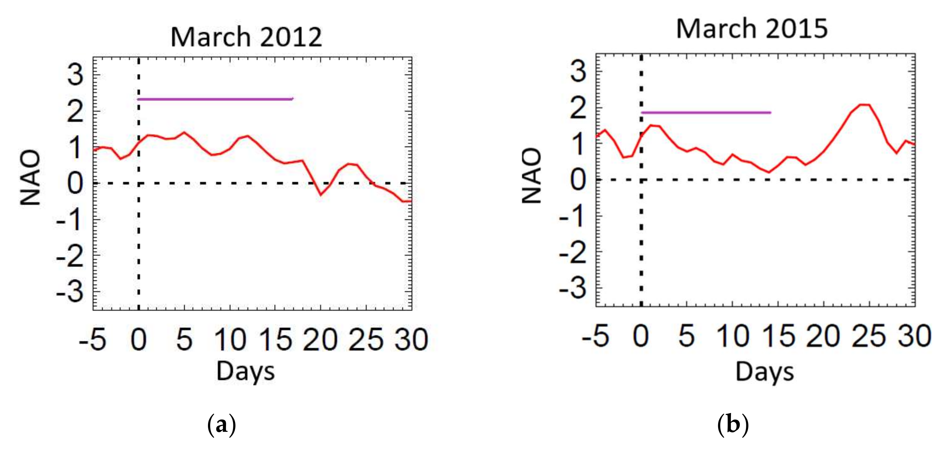
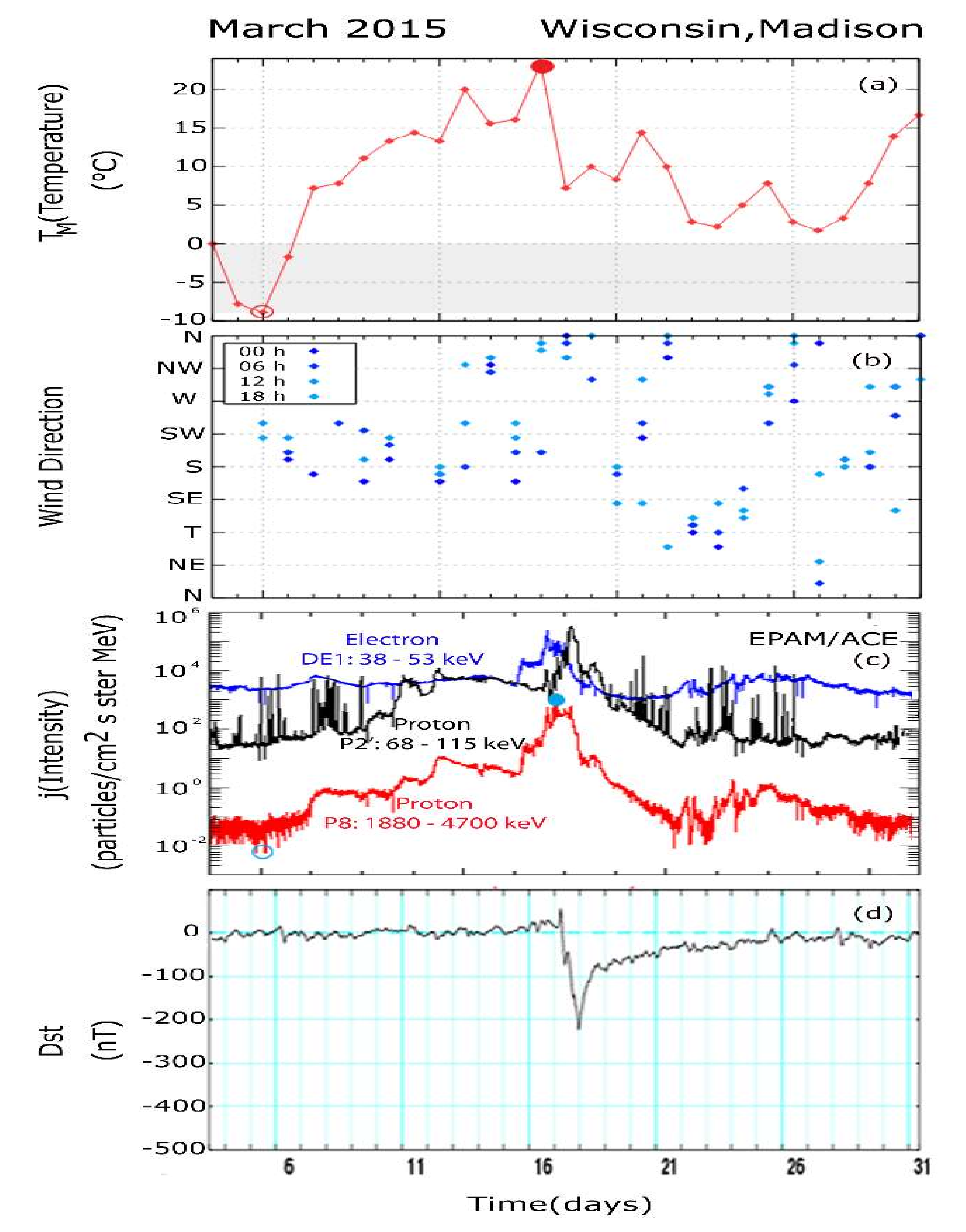
4.2. March 2015: An Event Similar to the March 2012 Event

In order to further check whether the temporal coincidence of the M2012HW with special solar and interplanetary activity was a coincidence or not, we proceed now to examine the atmospheric weather during the greatest (Dst = −223 nT) ICME storm of the weak solar cycle 24 [93], which occurred in March 2015, only 3 years after the March 2012 heat wave. This study follows the same strategy as the study of March 2012 events, as for instance, the comparison of ACE observations with near-ground air conditions in Madison, Wisconsin.

4.2.1. Solar and Interplanetary Conditions during the 2015 Heat Wave

Figure 6 has been constructed as Figure 3 but for the period 3–30 March 2015. In this figure, the time series has been centered around the time of the severe geomagnetic storm of 17 March 2015, the so-called Saint Patrick’s Day March 2015 magnetic storm, the largest magnetic storm throughout the solar cycle #24 (SC24). This superstorm reached values of the Dst index as large as −223 nT, and several studies have been devoted to understanding its origin on the Sun, their propagation in the interplanetary space and their interaction with both other IP structures and the geospace [94,95,96,97,98,99].

Two days before St Patrick’s Day, on 15 March 2015, the sunspot 2297 produced a C9.1 class flare with onset at 01:15 UT and peaking at 02:13 UT. There were several active regions on the visible face of the Sun in March 2015. The Solar Dynamics Observatory (SDO) image in the He II (304 Ångstrom) line detected a strong active region (AR2297) at 2304 UT on 14 March. By 0200 UT on 15 March, this region gave rise to a powerful CME event that was largely earthward directed [60,98]. Solar energetic particles began to flow around our planet in the early hours, on March 15, 2015, in a gradually increasing rhythm (Figure 6c).

According to WSA-ENLIL Solar Wind Prediction/NOAA, the impact of the ICME on the Earth’s atmosphere would occur on March 18, triggering a geomagnetic storm of only G1 (minor) level of intensity. However, at 04:10 UTC on 17 March 2015, 15 h earlier than expected, the ACE spacecraft detected the passage of an IP shock. Then, a period of enhanced geomagnetic activity began, reaching G3 (strong) to G4 (severe) geomagnetic conditions and was sustained for ≈12 h ([99]; their Figure 5).

C-flares are relatively common solar explosions and do not draw much attention. Although the solar active area was located to the west of the solar disk (S22, W29), that is, in a geoeffective location, the fast travel of the ICME to the Earth and the geoeffective strength of the March 15th ICME raised extensive scientific discussion [100,101,102,103,104,105].

The IP shock wave reached the Wind spacecraft at 03:59 UT, March 17, and the ACE spacecraft at 04:10 UT. Other observations obtained closer to the Earth show that the IP shock hit Earth’s magnetosphere a little later, at 04:45 UT on 17 March [60]; the time difference 04:45–04:10 UT, between the detection time at the Earth and at ACE, is due to the traveling time of the shock from the satellite to our planet. The ICME-related IP shock accelerated protons and electrons to high energies, which are seen as a distinct flux enhancement (≈8 × 10² p/(cm².sec.sr.MeV)), 15–17 March 2015 (panel c). The P8 high-energy (1880–4700 keV) proton data around the IP shock show a relative flux increase with a ratio p/b as high as ≈2.5 orders of magnitude compared to the proton fluxes on day 14 March (b ≅ 3 × 10⁰ p/(cm².sec.sr.MeV)), before the solar flare, and ≈4.5 orders of magnitude compared to the solar background on 5 March (b ≅ 4 × 10⁻²p/(cm².sec.sr.MeV)), before the whole SEP event.

The ACE data in Figure 6 show that the SEP event during 15–17 March is superimposed on the longer flux structure of the SEPI event lasting from March 6 to 7 or March 21. This long duration SEP event suggests an active Sun for several days around the March 17 shock arrival at the Earth. We can separate the energetic proton structure during 5–20 March into three distinct periods: (a) Period 1 (P1): the gradual flux increase lasting from its onset, on day 6, until the arrival of the ICME front, on March 15, (b) Period 2 (P2): the main SEP event observed from around the time of the CME generation until the arrival of the IP shock at the Earth’s environment (≈04:45 UT on 17 March), and Period 3 (P3): a relatively abrupt flux decrease on March 17 down to the pre-shock level (≈10¹ p/(cm².sec.sr.MeV) and a flux decay until 21 March 2015.

The 17 March 2015 IP shock resulted in a compression of the dayside magnetosphere and a prompt enhancement of relativistic electron flux in the outer magnetosphere, at L = 3–5, which was recorded by the Van Allen Probes Relativistic Electron Proton Telescope (REPT). The 17 March 2015 IP shock compression of the dayside magnetosphere and the subsequent inward motion of the magnetopause produced very strong events, with large electric field impulses, as observed in March 1991 and the Halloween 2003 storm, which are the most significant storms of the last 30 years. The large storm triggered acceleration processes which produced ultrarelativistic electrons up to ≈10 MeV [60]. Baker et al. [60] reported that the energized electrons in the outer radiation belt showed strong “butterfly” distributions throughout the storm with deep minima in flux at pitch angle α = 90°, which suggests the existence of energetic electron loss processing at those times. Electrons escaping from the outer radiation belt can precipitate in the atmosphere and produce the bright Aurora Borealis. Indeed, during the night of 17th March Aurora, lights were visible not only close to the poles, as in Alaska or Iceland, but people could see them as far south as Illinois, New York, and New Jersey.

From Figure 6, we see that the numerous short-lived spikes of low-energy protons were observed by ACE (at long distances from the Earth’s magnetosphere), during the recovery phase of the superstorm, between 19 and 26 March 2015 and they are obviously of a terrestrial origin (magnetosphere, bow shock). More specifically, the detection of “butterfly” electron distributions (minima in flux at pitch angle α = 90°) in the magnetosphere and the presence of the short time duration low-energy proton events during the recovery phase of the superstorm are consistent with energetic proton and electrons accelerating within the magnetosphere, which escaped into the interplanetary space, at the position of the ACE satellite. Furthermore, the large (10² < p/b < 10³) peak-to background flux ratio of the low-energy protons at far distances from the Earth [67] between days 22 and 26 confirms that strong acceleration processes were in progress within the Earth’s environment during the decay phase of the superstorm.

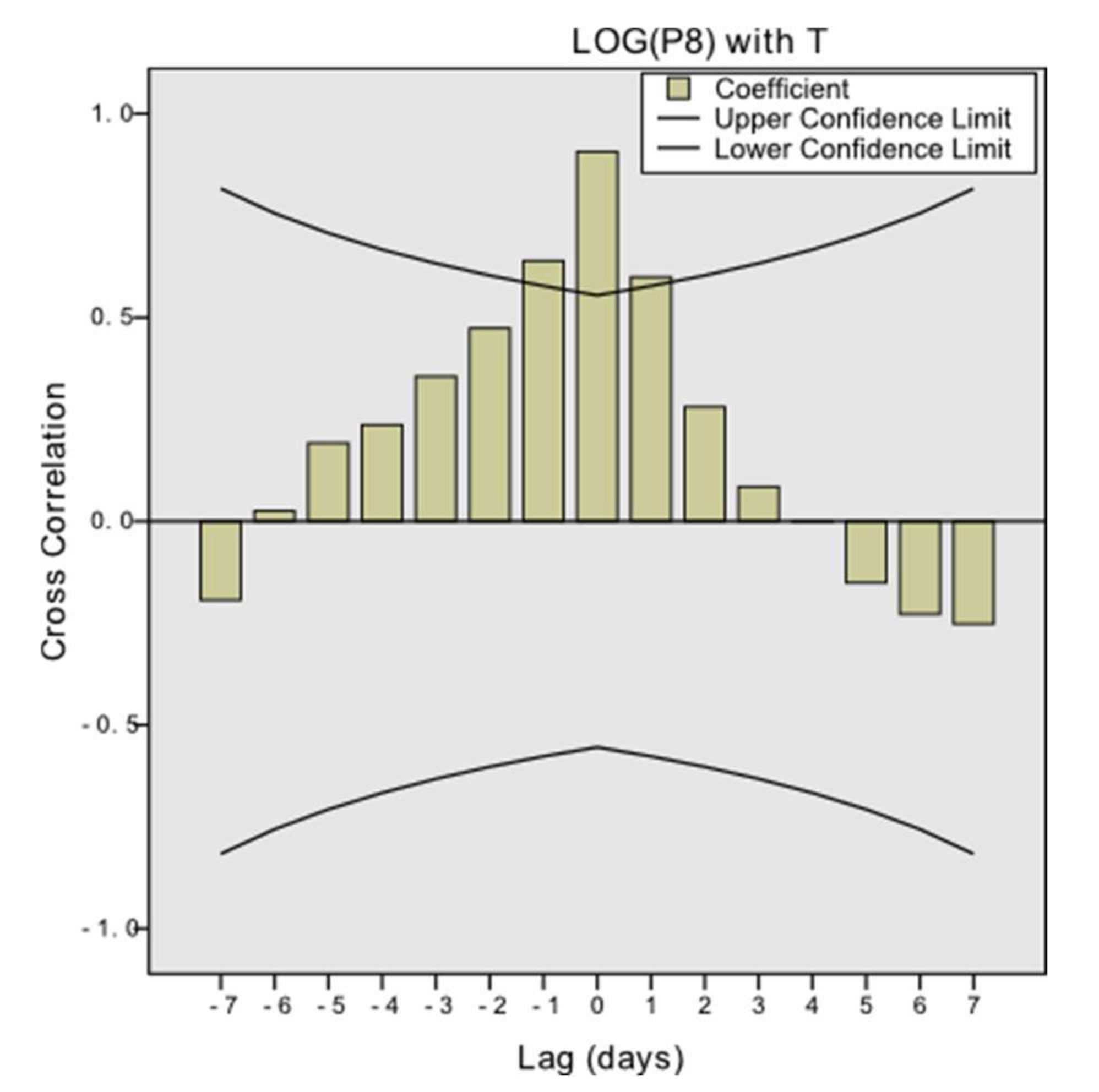
4.2.2. Atmospheric Weather during the March 2015 Heat Wave

We examine now the meteorological conditions in Madison, Wisconsin, during the period of March 2015 SEP event and the related superstorm. One of the most striking features of Figure 6 is the surprising resemblance of the profiles of the temperature in Madison, Wisconsin (panel a) and the 1.880–4.700 MeV (P8) solar proton flux (panel c) for about 2 weeks (6–21/22 March). Another striking result comes from the comparison of the temperature in Madison, Wisconsin, with near-ground air wind direction. From the comparison of panels a and b, we infer a relation between temperature and air wind direction in Madison such as that in the case of the March 2012 heat wave, i.e., a dependence of higher (lower) temperatures from the southward (northward) air streaming direction.

In particular, the following features can be observed during the time period examined in Figure 6: (i) We see that the long-lasting temperature anomaly in Madison starts and stops at (almost) the same time with the SEP event, that is on 6 and 22/23 March, respectively. (ii) During the period 6–22/23, we see, with the naked eye, a resemblance of values of two different physical parameters, which characterize two different physical magnitudes at distant regions, that is the flux of solar energetic particle in the distant interplanetary space and temperature of near-ground atmosphere. (iii) The peak temperature T_M, within the period examined in Figure 6 (3–31 March), occurred on March 17, that is on the same day as the arrival of the IP shock wave-associated P8 high-energy flux peak. (iv) The temperature T_M then reached a local maximum of 20 °C on day 13, and then, it fell to 150 C on day 14, in relation to the air wind streaming change from a southward to a northward direction. (v) During the decay phase P3 of the SEP event, that is after the IP shock of day 17 to days 22–23, while the T_M temperature decreased from 24 °C down to 20 °C, T_M showed a local maximum of 15 °C on day 19 after a daily southward wind streaming on day 18 and a 6 h interval on the same day (March 19).

The data in panels a and b demonstrate that between 6 and 16 March, during the increasing trend of the temperature T_M in Madison (panel b), the air wind streams from the general southward direction, except for day 7 when southern streaming was recorded for only a 6 h interval. On the contrary, we see that before day 6 (days 4–5) and after day 21, both the P8 proton flux and the temperature T_M in Madison show low values, while the air direction shows a fluctuating pattern with a varying flow direction.

Now, we evaluate computationally the relation of P8 and T_M between 6 and 16 March. In Figure 7 (adapted from Figure 2 of [8]), we present the estimates of the cross-correlation coefficients between the logarithm of the P8 proton flux values and the temperature T_M from day 6 until 16 and for lags 0, ±1, …, ±7. The upper and lower confidence limits are denoted with solid black lines.

From the evaluation of the cross-correlation coefficient, we found a very significant positive correlation at lags −1, 0 and 1. Especially at lag = 0, the cross-correlation coefficient takes its maximum value r = 0.907 with s.e. = 0.277 (p <0.001). This indicates that the daily increase in the temperature T_M was very well related with an analogous increase in the P8 high-energy proton flux. The very large r value, at lag = 0, confirms and explains the day-to-day simultaneous resemblance of the line plots of the temperature T_M and the P8 proton flux in Figure 6a,c. The p-value, being less than 0.001, suggests a very significant correlation between the two magnitudes, T_M and the P8, within a day. This very significant correlation strongly supports the concept that a very fast (<1 day) physical process mediated the space weather with the atmospheric weather in NE-USA in March 2015, under conditions of long duration–slow flux increasing of P8 high-energy protons.

The time coincidence of the long temperature anomaly with the whole SEP flux structure between 6 and 21 March and the similar profiles of temperature T_M in Madison, Wisconsin, with the solar energetic proton flux at a distance of ≈1.4 106 km from the Earth (ACE location) during the greatest superstorm of the SC24 suggests a very good correlation between ACE/P8 high-energy protons and T_M temperature during a period including the famous Saint Patrick’s Day (March 2015) events.

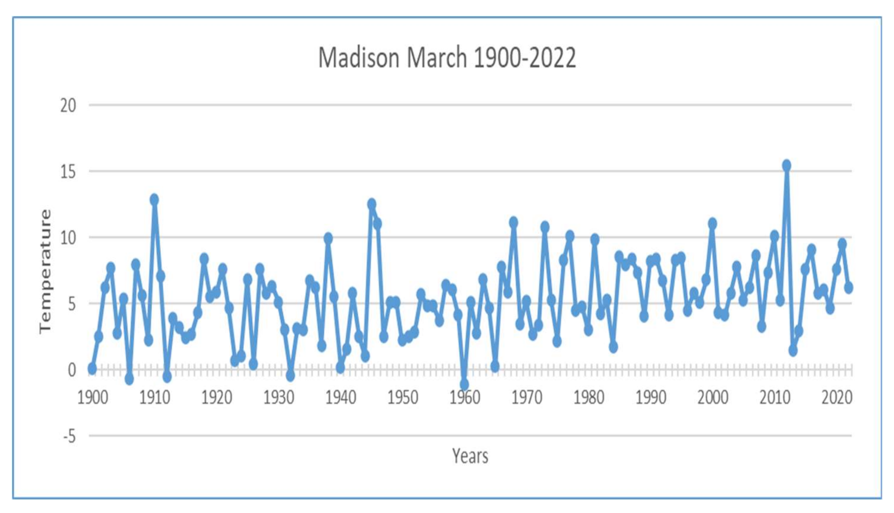
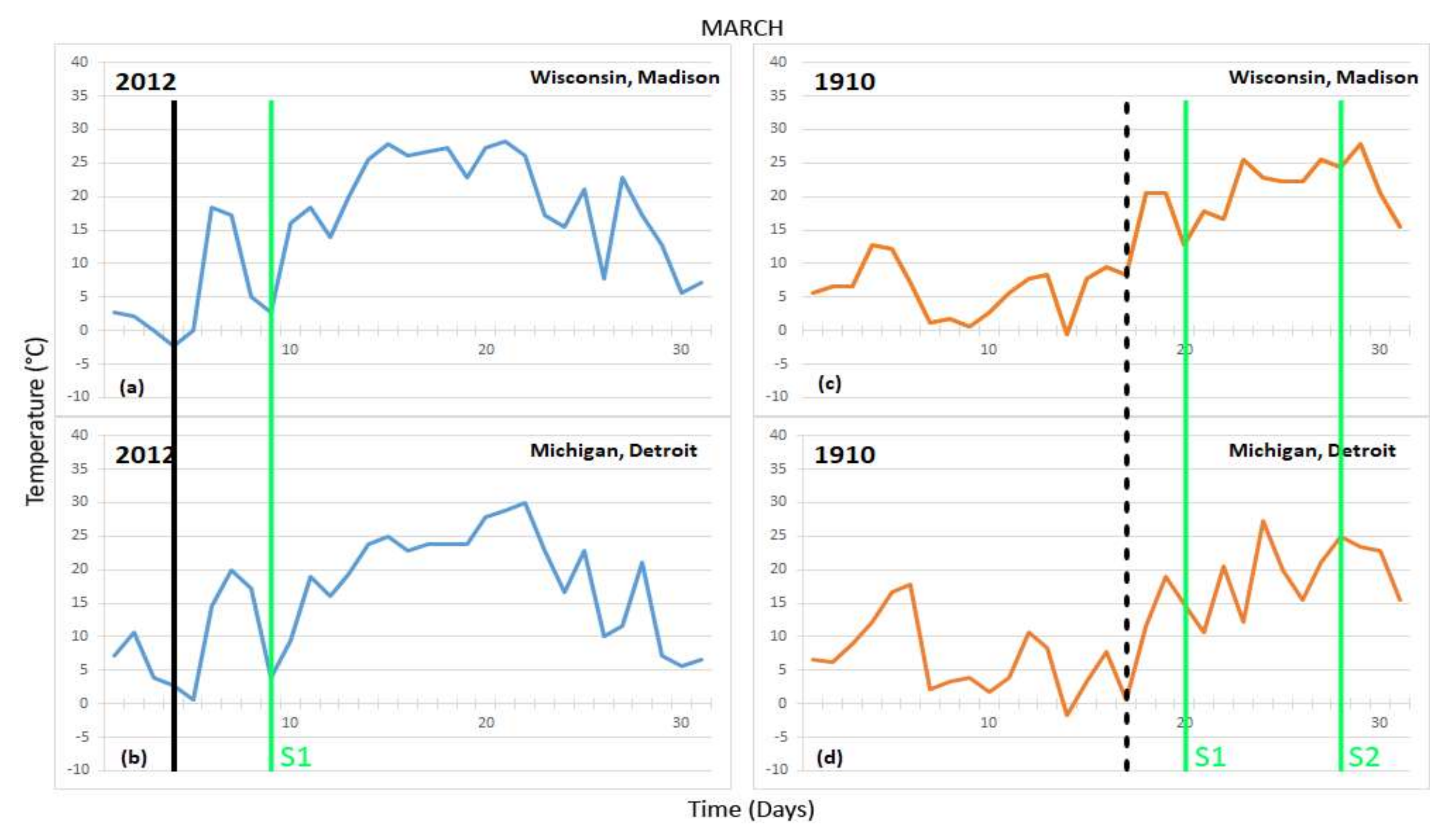
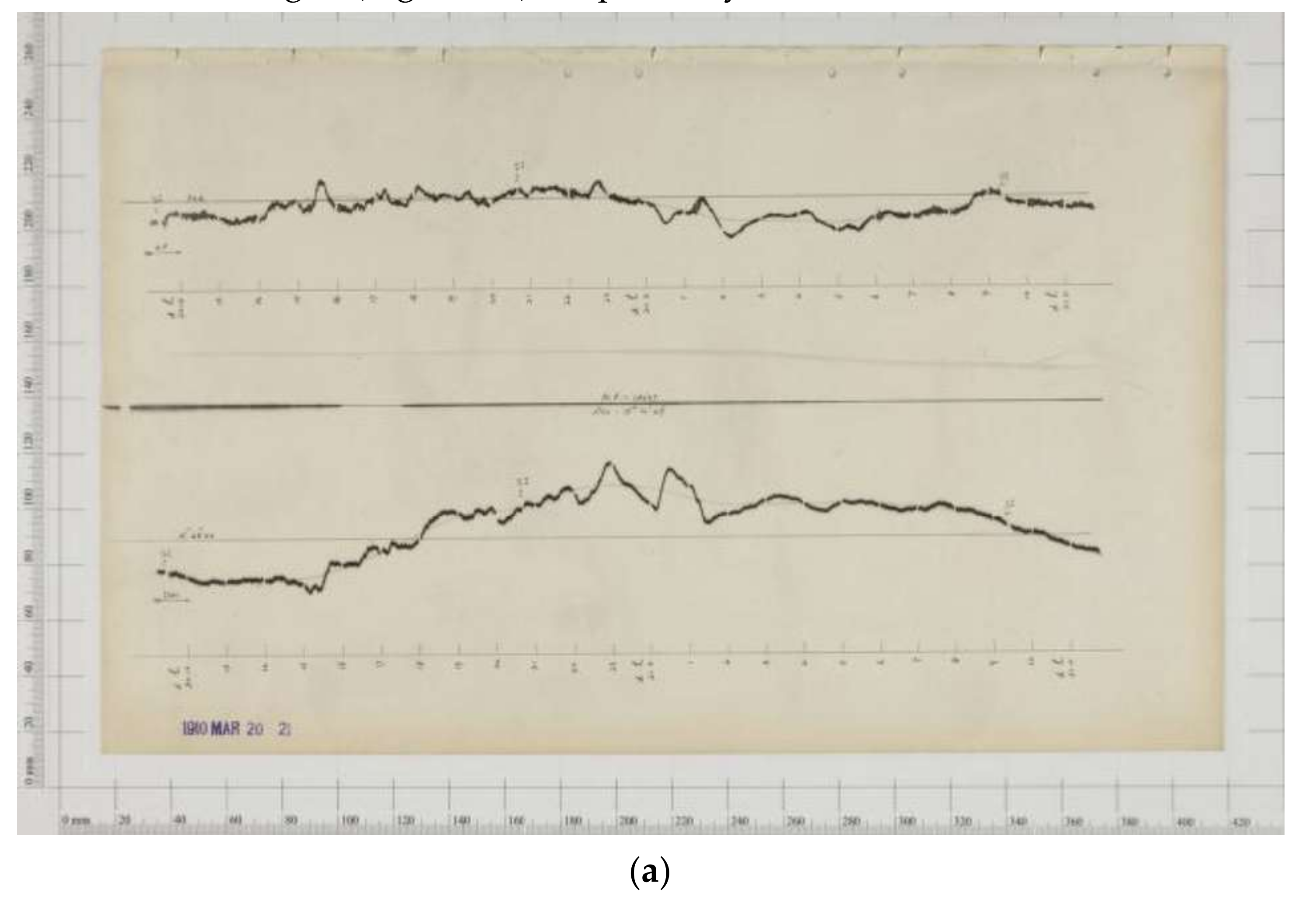
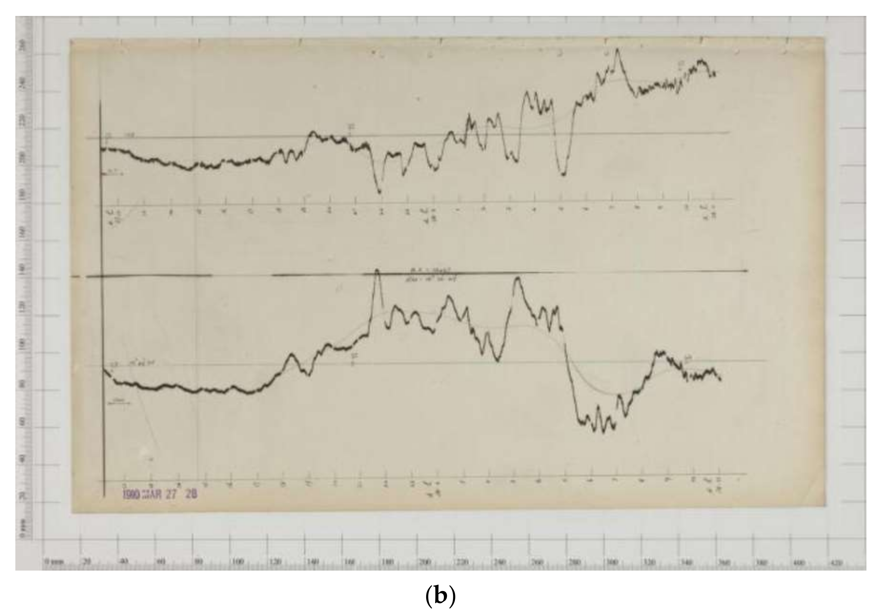
4.3. March 1910: An Earlier Comparable to the March 2012 Heat Wave

From panel c of Figure 6, we see that the temperature T_M in Madison increased within a period of 10 days (6–16 March) from −9 to 23 °C, that is a total increase as high as ΔT_M = 32 °C. The gradual temperature increase implies an average rate ΔT_M/Δt = 3.2 °C/day for 10 days. This temperature variation changed the Madison weather from a winter-type (−9 °C) to a summer-type one (+23 °C) at the beginning of March 2015. This temperature increase (ΔΤ = +32 °C) in Madison, Wisconsin, was the highest among the 28 events of Table A1 (Appendix A).

March of 1910 was the only month with a comparable but not such a striking heat wave as that of March 2012 (Figure 8). A NOAA report notes that March 1910 was the only month that had more than one 80-degree day in Sginaw, Michigan, when two non-consecutive 80° F (≈26 °C) days were recorded (https://www.weather.gov/dtx/unprecedentedmarchwarmth2012, accessed on 27 May 2022).

We have seen that the M2012HW followed a very active Sun. The historic heat wave coincided with an intense SEP event and a strong superstorm caused by the ICMEs (in the M2012HW as well). Many reports have noted the resemblance of M2012HW with the M1910HW. Therefore, the possible coincidence of M1910HW with solar activity, as in the case of M2012HW, would highly enlighten the discussion on the origin of both heat waves. The coincidence of M1910HW with solar activity would support the concept of a non-accidental coincidence of solar and atmospheric extreme events. (Figure 9)

However, we are not aware of any published research results checking the possible time coincidence of the M1910HW with solar activity. To this end, we checked the best signature of a solar effect on the Earth’s magnetic environment in the year 1910: any strong magnetic storms recorded in existing systematic historic databases. For this reason, we studied the magnetograms of March 1910 as opposed to 7 days (14–18, 20–22) in March 2012. Provided by the Greenwich Observatory (https://webapps.bgs.ac.uk/data/Magnetograms/search.cfc?method=magnetogramSearchbyObservatory, accessed on 27 May 2022). Figure 9 compares the time series of daily

In Figure 10, we show the magnetograms obtained from the Greenwich Observatory on 20–21 March 1910 (panel a) and 27–28 March 1910 (panel b), as provided by the British Geological Survey. The magnetograms show the H component of the magnetic field and its declination D. The magnetograms suggest the occurrence of two large magnetic storms starting on days 20 and 27 in March 1910, and they are indicated by the normal green lines S1 and S2 in the time series of temperature in Madison, Wisconsin (Figure 9c) and in Detroit, Michigan (Figure 9d), respectively.

Figure 9, in panels c and d show that the magnetic storm S1 proceeds the starting time (normal green dashed line) of M1910HW. A large magnetic storm is always due to a solar structure, which is characterized by a SEP event starting at least about 2 days before the magnetic storm; this is shown by the normal black lines in panels a and b, which indicate the onset time of March 2012 SEPI event. We can reasonably hypothesize that a SEP event occurred in March 1910 at almost the time indicated by the dashed normal black line.

5. Discussion

The possible influence of solar and space activity on air extreme weather was addressed in this study. The research on this topic has become of particular interest since people have experienced an exceptional number of unprecedented extreme weather events in the last decades, which have caused major human suffering and economic damage.

In particular, the March 2012 heat wave (M2012HW) in Northeast America was examined in this study based on a detailed comparison of solar/space and meteorological data in the context of previously published related studies.

The M2012HW was in general considered as a non-anthropogenic effect [3]. Scott [6] noted that “the heat wave that affected the eastern and central United States in March 2012 coincided with a flurry of solar eruptions, and it’s not unreasonable to wonder if such events are related. After all, the Sun’s energy is the source of Earth’s warmth”. However, the rejection of the hypothesis has been made on the basis of electromagnetic radiation in the spectral range from 1.27 to 17 µm (http://saber.gats-inc.com/, accessed on 1 June 2022) measured by SABER. However, this argument seems to accept that the only kind of solar energy affecting the Earth’s atmosphere comes from the electromagnetic radiation of solar activity and does not take into account the tremendous amounts of solar wind electromagnetic energy transferred by the ICMEs into the magnetosphere, with a power input >10¹² W, and that the percentage of the solar wind plasma energy that reached the Earth’s surface is still unknown.

Actually, March 2012 has become known for two extreme events in the environment of the Earth: first, for the historic heat wave in the United States and Canada and, second, for the great solar flare, the accompanied CMEs, the ICME-associated SEP event, the consequential magnetic superstorm, and magnetospheric particle dynamics, which have been extensively discussed in scientific papers, scientific web pages and newspapers.

Unfortunately, the March 2012 space and atmospheric events have been in general investigated as autonomous natural processes, without any examination of possible interaction, despite their time coincidence and their relative spatial vicinity (magnetosphere–ionosphere–atmosphere). It has been suggested that some natural phenomena, such as the Madden –Julian Oscillation, Atlantic Anomaly and North Atlantic Anomaly, were responsible for the M2012HW [2,3]; only a short reference has been made on the possible physical connection between space and atmospheric events [7,8].

March 2012 has been noted as the warmest on record since March 1910 (https://www.weather.gov/dtx/unprecedentedmarchwarmth2012, accessed on 27 May 2022).

The fact that the March 1910 heat wave occurred in 1910 in the United States, before the heavy anthropogenic burden of the Earth’s atmosphere over the last decades, pushed us to further examine the hypothesis that the March 2012 heat wave was triggered by some natural, non-anthropogenic phenomena. Dole et al. [3] attempted an interpretation of the “Meteorological March Madness” in terms of the concept of an autonomous terrestrial environment, but they considered a part of the whole event. (i) They studied the high temperatures only for the interval 12/14–23 March, and (ii) they noticed only the daily mean temperature increase of 15–20 °C above normal during March 12/14–23. In this way, their analysis did not take into account that (i) there is a single type of meteorological conditions between 4–23 March related with a varying air streaming direction and varying near-ground temperatures, (ii) the high-temperature period March 12/14–23 constitutes a phase of a longer (4–23 March) event, which is related with high-energy solar particle radiation, (iii) although it is true that March 2012 was an unusual heat wave because of daily mean temperatures of 15–20 °C above normal, it was actually a “Meteorological March Madness” rather because of the striking temperature increase from −20° to 28 °C (ΔΤ_M = 30 °C) between March 5 and 15 (Figure 3).

The rich scientific literature on solar–atmospheric relationships [40,41,42,43,44,47,48,49,50,51] and the fact that there was a temporal coincidence between extreme solar/space and atmospheric events during March 2012 provided us both with the challenge for further research and the observational basis for an extended examination of the hypothesis that solar activity might be a candidate physical factor influencing the M2012HW. To this end, in the present study, we examined in detail the relationship of several unusual solar, space and atmospheric records during March 2012.

Furthermore, we searched for any additional possible observational evidence for the solar–atmospheric physical connection during the March 2012 heat wave by gaining important information from a comparison with at least two more special heat waves: the historic March 1910 heat wave (a comparable heat wave about one century before March 2012) and the March 2015 heat wave (related with the largest ICME-related storm occurred in the same solar cycle 24 with M2012HW and investigated with exactly the same methodology/instrumentation).

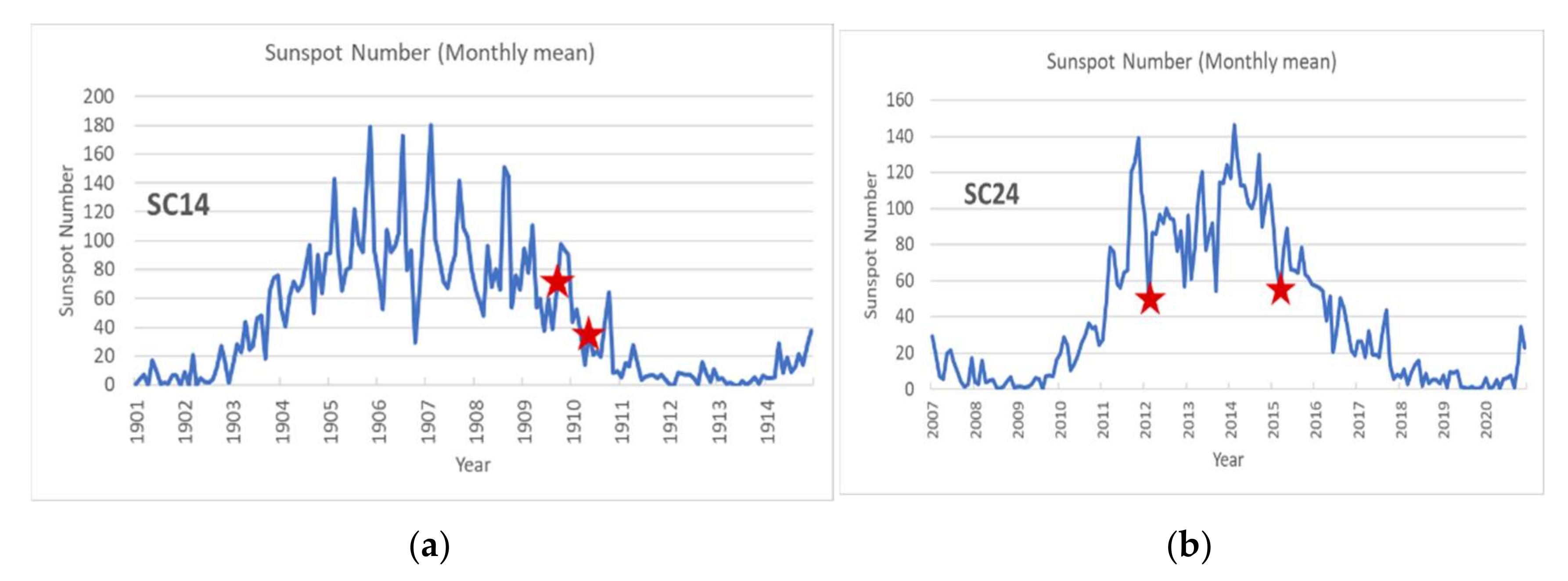
5.1. Unusual Solar/Space Activity before March 1910, March 2012 and March 2015 Heat Waves

Solar energetic particles are emitted during coronal mass ejections and solar flares, with particles mostly consisting of protons with energies from a few to several MeV. A very small portion of ICME-related SEP events extends to energies as high as E > 0.5 GeV, and they can reach the lower atmosphere at high and middle latitudes.

March 2012 and March 2015 SEP events (successive last events in Table A1, Appendix A) fall into the very special class of ICME-induced SEP events with the proton energy spectrum extending to energies E > 0.5 GeV, or, in other words, during times of CMEs, releasing high-energy solar cosmic rays in the interplanetary space.

Intense solar activity is known to have been restated with extreme atmospheric weather periods not only in the last decades but also before the GHG effect [21,105,106,107]. A previous extreme to the March 2012 heat wave is known to have occurred in March 1910 (Figure 8) in NE-USA (https://www.weather.gov/unprecendentwarmth2012 accessed on 27 May 2022) before the GHG effect, which suggests a non-anthropogenic effect for its origin. Since both the United States and the global surface temperature pattern during March 2012 were found to resemble the conditions observed during March 1910 ([3]; this paper, (Figure 9a,c versus Figure 9b,d) a common natural cause could be hypothesized for both the M1910HW and the March 1910 heat wave (M1910HW).

Our data analysis in the present paper reveals, for the first time, that the M1910HW in NE-USA (Wisconsin and Michigan) occurred during the detection of large magnetic storms, which were obviously related with high-speed solar wind streams and SEP events. It is worth noting that the magnetic storms related with the M1910HW occurred only a few months after the historic magnetic superstorm on 25 September 1909, with a Dst index attaining a minimum of −595 nT [21]. The violent September 1909 superstorm was one of the most intense CMEs of the 20th century, and it was comparable to that of the great 1859 Carrington event [107,108]. It caused telegraph disturbances, which were accompanied by auroral displays down to magnetic latitudes of 300 [100] in many parts of the world, such as in Western Australia and Scandinavia. Furthermore, it is remarkable that each of the M1910HW and M2012HW occurred during the two weaker solar cycles in the last 120 years, that is during SC14 and SC24, respectively (Figure 11c). As can be seen from Figure 11c, both heat waves resemble each other not only because of the weakness of the solar cycles 14 and 24 but also because of the highly variable solar activity, as can be revealed from the yearly averaged sunspot number (SSN) time series shown in Figure 11a,b (red asterisks: September 1909 CME and CMEs / heat waves in March 1910, March 2012 and March 2015.

Since the solar minimum phase of a weak solar cycle, such as SC14, is characterized by very high-speed solar streams emanating from highly enlarged solar holes and the historic September 1909 CME was released within a highly complex and disturbed IP medium, it is possible that a highly disturbed IP medium continued to be in progress and that, therefore, the heat wave in March 1910 most probably occurred under unusual space conditions (as for the storms in March 2012 and 2015). This an issue that would be interesting to further investigate in future studies.

Definitely, the fact that the two major March heat waves, the M1910HW and the M2012HW, which occurred a few days after large magnetic storms, are consistent with the concept that the two heat waves were influenced by similar extreme space conditions.

5.2. Solar–Space–Atmospheric Relationships in March 2012

Several physical mechanisms have been proposed to explain the possible links between solar wind, SEP events, magnetospheric activity, and changes in the stratosphere and the troposphere. Such mechanisms include (i) SEP relation with large stratospheric/tropospheric variations (i.e., pressure gradient causing downward airflow), (ii) variation in the global electric circuits, (iii) stratospheric ozone-related chemical energy changes, and (iv) charging of cloud droplets on the edges of layer clouds, which have recently been directly observed [109]. It is also possible that some of these mechanisms may operate in parallel.

Veretenenko et al. [110] noted that a regional character seems to be a characteristic feature of the lower atmosphere reaction to solar/geomagnetic activity influences caused by peculiarities of the atmospheric circulation in different regions. Disturbances of the lower atmospheric circulation associated with cosmic ray variations take place over the entire globe, with the processes developing in different latitudinal belts and regions being closely interconnected. The spatial structure of correlated pressure variations is closely related to their influence on the main elements of the large-scale atmospheric circulation, namely on the polar vortex, planetary frontal zones and extratropical cyclones and anticyclones [110]. In agreement with these results, March 2012 global meteorological anomalies observed during the ICME-related SEP events and magnetic storms have shown different features in various regions over the globe [3,7].

The study of meridional profiles of zonal atmospheric pressure during intense geomagnetic disturbances, including periods of SEPs and Forbush decreases of galactic cosmic rays, revealed that the observed variations in zonal circulation were due to the atmospheric processes at subpolar and polar latitudes (φ > 55⁰ N), i.e., they were characterized by a latitudinal dependence [49]. The latitudinal dependence of the zonal pressure spoke in favor of the hypothesis that cosmic rays’ variations were the most probable link between solar activity and the lower atmosphere. Later studies of short-period effects of cosmic rays variations in meteorological characteristics of the high-latitude atmosphere (Sodankylä station, Finland) carried out by Pudovkin’s team confirmed an important role of the variations in cosmic ray fluxes associated with solar activity in the disturbances of tropospheric circulation [106].

The North Atlantic Oscillation (NAO), an oscillation of atmospheric mass between the Arctic and the subtropical Atlantic, is one of the leading modes of climate variability in the northern hemisphere, where solar energetic particles have easier access. Scaife et al. [107] argued that stratospheric trends over the last few decades and the downward links to surface climate are strong enough to explain much of the prominent trend in the NAO and regional climate over Europe and North America between the 1960s and the 1990s.

The March 2012 and March 2015 heat waves in Northeast America occurred during a positive NAO index (Figure 5) and were strongly coupled to large-scale tropospheric poleward warm air transport (Figure 4 and Figure 8; [2,3]). The persistent southerly flow was confirmed as a key component in allowing an air mass of the Gulf of Mexico coastal region to be transported northward across the Great Lakes. The persistent southerly flow drew much of Gulf of Mexico moisture northward across Wisconsin, thus resulting in unseasonably humid conditions [2,3]. An additional finding of the present study is that the air surface was streaming from alternating directions within the time intervals examined (3–30, March 2012, 2015) in Madison/Wisconsin followed by temperature variations (low/high values), in such a way that temperature increases were related to large-scale tropospheric poleward warm air transport. We note that this feature was common for both the M2012HW and the M2015HW.

Significant evidence has been provided for a solar influence on NAO. Several studies have suggested a solar cycle correlation with NAO and large-scale tropospheric circulation systems [90]. Recent studies support the idea that solar activity influences tropospheric climate in the northern hemisphere via fluctuations of the stratospheric polar vortex.

Maliniemi et al. [103] found a statistically significant correlation between energetic electron precipitation in the upper ionosphere and the NAO index and also between energetic electron precipitation and surface air temperatures in three (winter) month-averaged data. However, enhanced energetic electron precipitation occurs during magnetic storms, and three-month-averaged electron flux increases are also consistent with high-energy proton presence due to solar SEP events related with storms.

The North Atlantic Oscillation on Northern Hemisphere Temperature occurs during wintertime from Florida to Greenland and from northwestern Africa over Europe [90,91,104]. It is remarkable that the March 2012 and March 2015 heat waves occurred during intense solar activity under positive NAO index in wintertime (March), with pre-heat temperatures as low as −2 °C in March 2012 and −9 °C in March 2015.

Most importantly for the Sun–atmospheric weather relationship is a strong short time (#days) relationship found between daily distribution of SSNs and NAO index [105]. The heat waves in March 2012 and March 2015, which occurred in North America during positive NAO (Figure 5) are consistent with the findings of the above studies.

In conclusion, according to the relative scientific literature a positive relation between NAO is expected (i) during strong solar activity, (ii) during winter, the positive NAO index is probably followed by large-scale tropospheric circulation. Indeed, the two heat waves we examined extensively occurred in wintertime (March 2012 and March 2015), in the presence of solar cosmic ray radiation; they were related to a positive NAO index followed by large-scale tropospheric variations (poleward warm air transport in Northeast America); although another physical mechanism may be responsible (or supplementary) for triggering the March 2012 and March 2015 large-scale tropospheric circulation in the North Atlantic, it is reasonable to assume NAO as a candidate mechanism as well [2].

Both heat waves during SC24 occurred during very unusual conditions. In particular, the great geoeffectiveness of the March 2012 superstorm was not expected on the basis of the solar flare source eastern site, since the sources of most major geomagnetic storms lie close to the central meridian. Moreover, the severe geomagnetic storm in March 2015, which was the largest in solar cycle 24, occurred without significant precursor X- or M-type solar flares, with the results that [95] titled their study “No Major Solar Flares but the Largest Geomagnetic Storm in the Present Solar Cycle, Space Weather”. Therefore, we may infer that the presence of high-energy solar cosmic rays (>0.5 GeV protons) and the highly disturbed and complex IP medium during both March 2012 and March 2015 provided appropriate extreme conditions, which enabled tropospheric dynamics to transfer large-scale warm air in northwest Atlantic regions.

6. Summary of Observations and Conclusions

The March 2012 historic heat wave (M2012HW) was characterized by some researchers as “Meteorological March Madness” or a “black swan event”. The present study focuses on the existence of the ongoing extreme space physical processes throughout the M2012HW and in particular the March 2012 ICME-related unusual SEP and geomagnetic events. The analysis of solar and space observations we conducted along with results from the relative published literature reveal a very complex and unusual space environment during the M2012HW. Some of its characteristic features are summarized below.

6.1. Space Observations

(1) Two extremely powerful flares occurred on 7 March 2012: the first one was a GOES X5.4 flare and the second one was a GOES X1.3 flare. These flares occurred after a flare from the same active region (AR 11429) on March 5. (2) In association with the two powerful flares, two ultra-fast CMEs with speeds as high as ≈2200 and 1800 km s⁻¹ were launched from the active region 11429 at east solar sites (E31° N18° and E26° N15°), which are normally not well connected with the Earth. (3) The IP medium, after the release of the two CMEs, was very complex and exhibited a non-extensive and non-Gaussian (Tsallis q-Gaussian) character [1]. (4) The March 7 CMEs-related shock(s) were so strong that they drifted much of the solar system [85]. (5) The SEP event on March 8 was (one of) the most intense events observed by the ACE satellite for a period of ≈18 years (1997–2015), with a peak-to-background (p/b) flux increase in the proton energy channel 1880–4700 keV as large as p/b > 5.5 × 10⁵ (Appendix A, Table A1). (6) The March 8 SEP event falls into a rare class of solar cosmic ray events with the energy spectrum extending to energies as high as E > ≈500 MeV (Figure 5, adapted from [37]). (7) A complex superstorm started on March 7, which was composed of four main IP shock-related storms. The last (4th) main storm occurred on March 15, but the whole superstorm showed a recovery on ≈22 March. The extreme IP plasma characteristics were responsible for the overall complexity of the magnetosphere (Section 4.1.3; [1,79,97]). The strong geoeffectiveness was unpredictable on the basis of the two CMEs generated on the east Sun (E31° N18°, E26° N15°). (8) Very high solar wind speeds were observed for long time intervals related with a magnetosonic Mach number of ≈9.4, which is the largest in recorded history [79]. (9) During the dipolarization of the magnetic field on March 9th, distinct electron injection events in the inner magnetosphere were followed by electron precipitation in the high-latitude ionosphere of the cusp, observed by the NOAA-18 satellite with fluxes >2 order of magnitude above the flux level of the solar electron ambient population. The electron precipitation was so strong during the main storm of March 9 (Figure 4) that the slot region between the inner and the outer radiation belt almost disappeared. (9) The largest (Dst = −222 nT) magnetic storm of SC24 occurred in March 2015 only three years after the M2012HW, and it was also related to a heat wave in the Northeast United States. The space conditions at those times, in general, resemble those of the March 2012 heat wave: the magnetic storm was caused by an unexpected geoeffective ICME, and its associated SEP event was characterized by a proton spectrum extending to very high (>0.5 GeV) energies, while the NAO index remained in a positive-value phase. (10) The M2012HW and the M2015HW occurred during a very weak solar cycle (SC14). (11) Two large magnetic storms occurred during March 1910, which was the warmest March in USA history before March 2012.

6.2. Meteorological Observations

(1) Positive NAO indexes were recorded during the M2012HW and the M2015HW. (2) Large-scale warm air mass was streaming from southern latitudes during times of high temperatures in NE-USA during the two heat waves (confirmed as originated from the Gulf of Mexico coastal in the case of the M2012HW [2,3]). (3) Almost simultaneous onset of the SEP and the temperature increase in daily averaged data was found in both cases, the M2012HW and the M2015HW. (4) There were extremely huge temperature increases ΔΤ_Μ = 30° and 32°, with maximum temperatures Τ_Μ = 28° and 23° achieved from pre-event levels as low as −2 °C and −9 °C M2012HW and the M2015HW. (5) (6) At the beginning of M2012HW, the temperature Τ_Μ suddenly increased from −2 °C, on March 4, to ≈18 °C, on March 6. (6) An unusual long duration of high daily temperatures Τ_Μ was recorded in Madison, Wisconsin, in March 2012; Τ_Μ ranged ≈23–28 °C for one week and remained at levels > 16 °C for a total time of ≈2 weeks. (7) A gradual increasing rate of daily maximum temperature Τ_Μ was recorded with a variation of 32 °C within 10 days with an average rate ΔT_M/Δt = 3.2 °C/day in March 2015. (8) Very strong and significant (r = 0.907, p < 0.001) correlation was evaluated between the near-ground air temperature and the ACE high-energy (1.880–4.700 MeV) proton flux during the 10-day period of their gradual increase. (9) The long-lasting simultaneous gradual increase in both the near-ground air temperature and the ACE high-energy proton flux occurred before the related superstorm. (10) The unusual long duration of high daily temperatures were recorded in NE-USA a century earlier, in March 1910, with daily maximum temperatures Τ_Μ = ≈25.5 °C and ≈28 °C on March 23/25 and 29, respectively.

6.3. Solar Activity and Heat Wave in March 1910, 2012 and 2015

(1) During the historic M2012HW, the ground air temperature recorded the highest levels since the M1910HW. (2) The M1910HW occurred before the greenhouse gases effect. (3) Both the local (United States) and the global surface temperature pattern during March 2012 have a historical resemblance to conditions observed in March 1910 ([3]; Figure 9b,d). (4) The March 2012 and the March 2015 heat waves occurred during times of solar activity causing unusual complex interplanetary conditions. (5) The M2012HW and the M2015HW occurred in the presence of high-energy solar cosmic rays (E > 0.5 GeV). (6) The ICME-related SEP events in March 2012 and the March 2015 caused strong magnetic superstorms accompanied by unusual strong electron precipitation in the high-latitude ionosphere. (7) Since the M1910HW occurred under large magnetic storms, it is inferred that all three distinct heat waves occurred under special space weather conditions. (8) All three heat waves occurred during the two weakest solar cycles in the last 120 years: solar cycles 14 (M10910HW) and 24 (M2012HW, M2015HW).

The influence of solar activity on the Earth’s climate is a well-known and generally accepted phenomenon. Furthermore, Earth-based and satellite measurements have shown that ICMEs affect the stratospheric and the tropospheric weather. Variations in the air temperature and the atmospheric pressure have been confirmed, during the extreme solar activity, in the low altitude troposphere, down to 2100 m above sea level [43]. In the present paper, we investigated in depth, for the first time, the possible solar influence on the near-ground weather extremes.

In particular, we examined the possible influence of solar activity on the historic M2012HW in NE-USA (Madison, Wisconsin). To this end, we also studied two more March heat waves in the same region. Our data analysis demonstrated that the M2012HW and the heat wave during the largest storm of the same solar cycle C24, in March 2015, occurred under unusual solar and interplanetary conditions.

The M2012HW and M2015HW have shown many striking similarities but also some differences. The heat waves in March 2012 and March 2015 have shown comparable large temperature increases, ΔΤ_Μ = 30° and 32°, respectively, under similar extreme space conditions, as for instance, they both occurred after the onset of intense SEP events, in relation with unexpected geoeffective ICMEs causing large and complex magnetic superstorms, under a positive NAO index and in the presence of large-scale warm air streaming from southern latitudes, while the most striking common space features seems to be the presence of high-energy (0.5 GeV) solar cosmic rays. Although M2012HW and M2015HW started from different pre-SEP temperature levels (−2 °C versus −9 °C), they lasted for different time intervals, and their related SEP events showed different temporal profiles and a much different time relation to the storm. It is also worth noting that the maximum ACE proton fluxes in the energy channel 1880–4700 keV was higher by ≈2 orders of magnitude during the March 2012 SEP than those during the March 2015 SEP, while the maximum flux values of the March 2012 SEP event was the highest flux observed during the 28 largest (Dst > −150 nT) storms during ≈18 year (Table A1; Appendix A).

The M2012HW and the M1910HW were characterized by similar local (United States) and global surface temperature patterns [3], and they were related to large magnetic storms. The comparable heat wave to the M2012HW, but also weaker, heat wave of March 1910, in the same region (NE-USA) occurred during intense geomagnetic activity. We infer, therefore, that all three distinct heat waves (M2012HW, M2015HW, M1910HW) we examined in this study occurred after the influence of Sun originated special plasma structures, which also caused strong magnetic storms.

Furthermore, the three heat waves, which occurred during SC14 (M1910HW) and SC24 (M2012HW, M2015HW), which were the weakest solar cycles during the last 120 years, may suggest some occurrence preference of these events for weak solar cycles, although no solid conclusion can be made on the basis of only three events. During weak solar cycles, the coronal holes enlarge, very high-speed solar wind streams emanate from the Sun, and complex interplanetary structures are observed in the presence of strong CMEs, as in the cases of March 2012 and 2015 CMEs confirmed by a series of satellites [1,76,77,78,82,85].

The M1910HW occurred before the GHG effect, and it should be understood as a natural, non-anthropogenic event. On the other hand, all three heat waves examined here were related with strong magnetic storms triggered by effective solar wind plasma structures. We infer that these results are consistent with the concept of a solar/space weather influence on the heat waves in March 2012, 2015 and 1910 in NE-USA.

In addition to the solar high-energy (>0.5 GeV) protons, which seem to play a major role on the solar influence on M2012HW and M2015HW, high-speed solar wind streams and strong magnetospheric electron precipitation were observed during the March 2012 and March 2015 superstorms, which may have been contributing factors for the generation of the large-scale warm air flows from the Gulf Mexico to NE-USA and Canada. Since the long-lasting highly correlated gradual increase in the near-ground air temperature and the ACE high-energy proton flux occurred in March 2015 before the related superstorm, a predominance of the solar component on the magnetospheric one is inferred if a space influence on the M2015HW is assumed.

Furthermore, it is possible that the observed differences in the solar proton streaming (flux level, flux rate increase) toward the planet Earth and in the pre-SEP temperature levels in the region considered (Madison, Wisconsin) affected the appearance of a stronger heat wave in March 2012 than in March 2015; definitely, the occurrence of the two major heat waves in March 2012 and March 1910 under highly disturbed space conditions open a new insight into understanding the origin of the M2012HW.

The present study has been further extended to a statistical one in order to search for any possible solar–weather relationships during a period of ≈18 years (from the beginning of the ACE satellite in the year 1997 until the year 2015; Table A1, Appendix A). We compared great magnetic storms (Dst < −115), ACE observations, and air ground weather in two different regions on the globe: the Northeast United States (Madison, Wisconsin) and Southeast Europe (Athens, Thessaloniki/Greece). The results of our data analysis will be presented in a future paper, which is under final preparation. This study suggests different patterns on the solar–ground weather relationships in the Northeast United States and Southeast Europe, with preferential dry-warm and wet-cold weather, respectively. In the same study, we analyze in depth the relation between solar activity–extreme (bad) weather in Greece during the period of M2012HW in NE-USA, and we distinguish between electric field anomalies due to different agents (during rainstorms versus geomagnetic storms).

The present study is the first one that elaborates the relation of simultaneous space and near-ground extreme weather (heat wave) events and their possible physical connection. We believe that the observations presented and discussed here suggest that we cannot reject the hypothesis of a solar influence on the March 2012 heat wave. Of course, more work is needed to further check the March 2012 space and atmospheric events. Finally, we think that a multi-point data comparison along with a detailed theoretical framework are needed to better explain the extreme space–atmosphere weather interaction in the light shed by the present results.

References

1. Patsourakos, S.; Georgoulis, M.K.; Vourlidas, A.; Nindos, A.; Sarris, T.; Anagnostopoulos, G.; Anastasiadis, A.; Chintzoglou, G.; Daglis, I.A.; Gontikakis, C.; et al. The major geoeffective Solar eruptions of 2012 March 7: Comprehensive Sun-to-Earth analysis. Astrophys. J. 2016, 817, 14. [Google Scholar] [CrossRef]
2. Borth, S.; Castro, R.; Birk, K. The Historic March 2012 Heat Wave: A Meteorological Retrospective. Available online: https://www.weather.gov/media/lot/events/March2012/March_Heatwave_2012_final.pdf (accessed on 1 March 2022).
3. Dole, R.; Hoerling, M.; Kumar, A.; Eischeid, J.; Perlwitz, J.; Quan, X.-W.; Kiladis, G.; Webb, R.; Murray, D.; Chen, M.; et al. The making of an extreme event: Putting the Pieces Together. Bull. Am. Meteorol. Soc. 2014, 95, ES57–ES60. [Google Scholar] [CrossRef]
4. Grumm, R.H.; Arnott, J.M.; Halblaub, J. The Epic Eastern North American Warm Episode of March 2012. J. Oper. Meteor 2014, 2, 36–50. [Google Scholar] [CrossRef]
5. Ellwood, E.R.; Temple, S.A.; Primack, R.; Bradley, N.L.; Davis, C. Record-Breaking Early Flowering in the Eastern United States. PLoS ONE 2013, 8, e53788. [Google Scholar] [CrossRef]
6. Scott, M. Do Solar Storms Cause Heat Waves on Earth? Available online: https://www.climate.gov/news-features/climate-qa/do-solar-storms-cause-heat-waves-earth (accessed on 29 March 2022).
7. Anagnostopoulos, G.C. Correlation between Space and Atmospheric March 2012 Extreme Events. In Proceedings of the EGU General Assembly Conference Abstracts, Vienna, Austria, 22–27 April 2012; p. 14048. [Google Scholar]
8. Anagnostopoulos, G.; Menesidou, S.A.; Vassiliadis, V.; Rigas, A. Correlation between Solar Particles and Temperature in North-East USA. In Proceedings of the 12th Hel.A.S Conference, Thessaloniki, Greece, 28 June–2 July 2015. [Google Scholar]
9. Herman, J.R.; Goldberg, R.A. Sun, Weather, and Climate; Dover Pub. Inc.: New York, NY, USA, 1978. [Google Scholar]
10. Coumou, D.; Rahmstorf, S. A Decade of Weather Extremes. Nat. Clim. Chang. 2012, 2, 491–496. [Google Scholar] [CrossRef]
11. Shindell, D.T.; Schmidt, G.A.; Mann, M.E.; Rind, D.; Waple, A. Solar Forcing of Regional Climate Change during the Maunder Minimum. Science 2001, 294, 2149–2152. [Google Scholar] [CrossRef] [Green Version]
12. Easterbrook, D. The Solar Magnetic Cause of Climate Changes and Origin of the Ice Ages, 3rd ed.Indepedently Publisher: Washington, DC, USA, 2019. [Google Scholar]
13. Robine, J.-M.; Cheung, S.L.K.; Roy, S.L.; Oyen, H.V.; Griffiths, C.; Michel, J.-P.; Herrmann, F.R. Death Toll Exceeded 70,000 in Europe during the Summer of 2003. Comptes Rendus Biol. 2008, 331, 171–178. [Google Scholar] [CrossRef]
14. CarbonBrief, Attributing Extreme Weather to Climate Change. Available online: https://www.carbonbrief.org/mapped-how-climate-change-affects-extreme-weather-around-the-world (accessed on 1 March 2022).
15. Wilcke, R.A.I.; Kjellström, E.; Lin, C.; Matei, D.; Moberg, A.; Tyrlis, E. The Extremely Warm Summer of 2018 in Sweden—Set in a Historical Context. Earth Syst. Dyn. 2020, 11, 1107–1121. [Google Scholar] [CrossRef]
16. Pascale, S.; Kapnick, S.B.; Delworth, T.L.; Cooke, W.F. Increasing Risk of Another Cape Town “Day Zero” Drought in the 21st Century. Proc. Natl. Acad. Sci. USA 2020, 117, 29495–29503. [Google Scholar] [CrossRef]
17. Sjoukje, F.; Sparrow, S.; Kew, S.F.; van der Wiel, K.; Wanders, N.; Singh, R.; Hassan, A.; Mohammed, K.; Javid, H.; Haustein, K.; et al. Attributing the 2017 Bangladesh Floods from Meteorological and Hydrological Perspectives. Hydrol. Earth Syst. Sci. 2019, 23, 1409–1429. [Google Scholar] [CrossRef] [Green Version]
18. Keellings, D.; Hernández Ayala, J.J. Extreme Rainfall Associated With Hurricane Maria Over Puerto Rico and Its Connections to Climate Variability and Change. Geophys. Res. Lett. 2019, 46, 2964–2973. [Google Scholar] [CrossRef]
19. Dole, R.; Hoerling, M.; Perlwitz, J.; Eischeid, J.; Pegion, P.; Zhang, T.; Quan, X.-W.; Xu, T.; Murray, D. Was There a Basis for Anticipating the 2010 Russian Heat Wave? Geophys. Res. Lett. 2011, 38, L06702. [Google Scholar] [CrossRef] [Green Version]
20. Kumar, A.S.; Chen, M.; Hoerling, M.; Eischeid, J. Do Extreme Climate Events Require Extreme Forcings. Geophys. Res. Lett. 2013, 40, 3440–3445. [Google Scholar] [CrossRef]
21. Love, J.; Hayakawa, H.; Cliver, E. On the Intensity of the Magnetic Superstorm of September 1909. Space Weather 2019, 17, 37–45. [Google Scholar] [CrossRef] [Green Version]
22. Mueller, B.; Seneviratne, S.I. Hot Days Induced by Precipitation Deficits at the Global Scale. Proc. Natl. Acad. Sci. USA 2012, 109, 12398–12403. [Google Scholar] [CrossRef] [Green Version]
23. Connolly, R.; Soon, W.; Connolly, M.; Baliunas, S.; Berglund, J.; Butler, C.J.; Cionco, R.G.; Elias, A.G.; Fedorov, V.M.; Harde, H.; et al. How Much Has the Sun Influenced Northern Hemisphere Temperature Trends? An Ongoing Debate. Res. Astron. Astrophys. 2021, 21, 131. [Google Scholar] [CrossRef]
24. Raspopov, O.; Veretenenko, S. Solar Activity and Cosmic Rays: Influence on Cloudiness and Processes in the Lower Atmosphere (in Memory and on the 75th Anniversary of M.I. Pudovkin). Geomagn. Aeron. 2009, 49, 137–145. [Google Scholar] [CrossRef]
25. Desai, M.; Giacalone, J. Large Gradual Solar Energetic Particle Events. Living Rev. Sol. Phys. 2016, 13, 3. [Google Scholar] [CrossRef] [Green Version]
26. Manchester, W.; Kilpua, E.K.J.; Liu, Y.D.; Lugaz, N.; Riley, P.; Török, T.; Vršnak, B. The Physical Processes of CME/ICME Evolution. Space Sci. Rev. 2017, 212, 1159–1219. [Google Scholar] [CrossRef] [Green Version]
27. Lamy, P.L.; Floyd, O.; Boclet, B.; Wojak, J.; Gilardy, H.; Barlyaeva, T. Coronal Mass Ejections over Solar Cycles 23 and 24. Space Sci. Rev. 2019, 215, 39. [Google Scholar] [CrossRef] [Green Version]
28. Axford, W.I.; Leer, E.; Skadron, G. The Acceleration of Cosmic Rays by Shock Waves. In Proceedings of the International Cosmic Ray Conference, Plovdiv, Bulgaria, 13–26 August 1977; Volume 11, p. 132. [Google Scholar]
29. Kallenrode, M.-B. Current Views on Impulsive and Gradual Solar Energetic Particle Events. J. Phys. G Nuclear Part. Phys. 2003, 29, 965–981. [Google Scholar] [CrossRef]
30. Armstrong, T.P.; Pesses, M.E.; Decker, R.B. Shock Drift Acceleration. In Collisionless Shocks in the Heliosphere: Reviews of Current Research; American Geophysical Union: Washington, DC, USA, 1985; p. 271. ISBN 978-1-118-66417-9. [Google Scholar]
31. Anagnostopoulos, G.C. Dominant Acceleration Processes of Energetic Protons at the Earth’s Bow Shock. Phys. Scr. 1994, 52, 142–151. [Google Scholar] [CrossRef]
32. Sarris, E.T.; Anagnostopoulos, G.C.; Trochoutsos, P.C. On the E-W Asymmetry and the Generation of ESP Events. Sol. Phys. 1984, 93, 195–210. [Google Scholar]
33. Cane, H.V.; Reames, D.V.; von Rosenvinge, T.T. The Role of Interplanetary Shocks in the Longitude Distribution of Solar Energetic Particles. J. Geophys. Res. Space Phys. 1988, 93, 9555–9567. [Google Scholar] [CrossRef]
34. Ryan, J.M.; Lockwood, J.A.; Debrunner, H. Solar Energetic Particles. Space Sci. Rev. 2000, 93, 35–53. [Google Scholar] [CrossRef]
35. Mavromichalaki, H. The physics of cosmic rays applied to space weather. In Advances in Solar and Solar-Terrestrial Physics; Research Signpost: Trivandrum, India, 2012; pp. 135–161. ISBN 978-81-308-0483-5. 37/661 (2). [Google Scholar]
36. Souvatzoglou, G.; Papaioannou, A.; Mavromichalaki, H.; Dimitroulakos, J.; Sarlanis, C. Optimizing the Real-Time Ground Level Enhancement Alert System Based on Neutron Monitor Measurements: Introducing GLE Alert Plus. Space Weather 2014, 12, 633–649. [Google Scholar] [CrossRef]
37. Kühl, P.; Dresing, N.; Heber, B.; Klassen, A. Solar Energetic Particle Events with Protons Above 500 MeV Between 1995 and 2015 Measured with SOHO/EPHIN. Sol. Phys. 2017, 292, 10. [Google Scholar] [CrossRef] [Green Version]
38. Gray, L.J.; Beer, J.; Geller, M.; Haigh, J.D.; Lockwood, M.; Matthes, K.; Cubasch, U.; Fleitmann, D.; Harrison, G.; Hood, L.; et al. Solar Influence on Climate. Rev. Geophys. 2010, 48, RG4001. [Google Scholar] [CrossRef]
39. Labitzke, K.; Kunze, M.; Brönnimann, S. Sunspots, the QBO and the Stratosphere in the North Polar Region 20 Years Later. Meteorol. Z. 2006, 15, 355–363. [Google Scholar] [CrossRef]
40. Schuurmans, C.J.E. Tropospheric Effects of Variable Solar Activity. Sol. Phys. 1981, 74, 417–419. [Google Scholar] [CrossRef]
41. Pudovkin, M.I. Influence of Solar Activity on the Lower Atmosphere State. Int. J. Geomagn. Aeron. 2004, 5, GI2007. [Google Scholar] [CrossRef]
42. Siingh, D.; Singh, R.P.; Singh, A.K.; Kulkarni, M.N.; Gautam, A.S.; Singh, A.K. Solar Activity, Lightning and Climate. Surv. Geophys. 2011, 32, 659. [Google Scholar] [CrossRef]
43. Avakyan, S.V.; Voronin, N.A.; Nikol’sky, G.A. Response of Atmospheric Pressure and Air Temperature to the Solar Events in October 2003. Geomagn. Aeron. 2015, 55, 1180–1185. [Google Scholar] [CrossRef]
44. Le Mouël, J.-L.; Lopes, F.; Courtillot, V. A Solar Signature in Many Climate Indices. J. Geophy. Res. Atmos. 2019, 124, 2600–2619. [Google Scholar] [CrossRef]
45. Kossobokov, V.; Mouël, J.L.; Courtillot, V. On the Diversity of Long-Term Temperature Responses to Varying Levels of Solar Activity at Ten European Observatories. Appl. Categ. Struct. 2019, 9, 498–526. [Google Scholar] [CrossRef] [Green Version]
46. Vourlidas, A.; Balmaceda, L.A.; Stenborg, G.; Lago, A.D. Multi-Viewpoint Coronal Mass Ejection Catalog Based on STEREO COR2 Observations. Astrophys. J. 2017, 838, 141. [Google Scholar] [CrossRef]
47. Schuurmans, C.J.E.; Oort, A.H. A Statistical Study of Pressure Changes in the Troposphere and Lower Stratosphere after Strong Solar Flares. Pure Appl. Geophys. 1969, 75, 233–246. [Google Scholar] [CrossRef]
48. Pudovkin, M.I.; Raspopov, O.M. A mechanism of solar activity influence on the state of the lower atmosphere and meteoparameters. Geomagn. Aeron. 1992, 32, 1–9. [Google Scholar]
49. Pudovkin, M.I.; Babushkina, S.V. Influence of Solar Flares and Disturbances of the Interplanetary Medium on the Atmospheric Circulation. J. Atmos. Terr. Phys. 1992, 54, 841–846. [Google Scholar] [CrossRef]
50. Fröhlich, C.; Lean, J. Solar Radiative Output and Its Variability: Evidence and Mechanisms. Astron. Astrophys. Rev. 2004, 12, 273–320. [Google Scholar] [CrossRef]
51. Smirnov, S.E.; Mikhailova, G.A.; Kapustina, O.V. Variations in Electric and Meteorological Parameters in the Near-Earth’s Atmosphere at Kamchatka during the Solar Events in October 2003. Geomagn. Aeron. 2014, 54, 240–247. [Google Scholar] [CrossRef]
52. Mironova, I.A.; Usoskin, I.G. Possible Effect of Strong Solar Energetic Particle Events on Polar Stratospheric Aerosol: A Summary of Observational Results. Environ. Res. Lett. 2014, 9, 015002. [Google Scholar] [CrossRef] [Green Version]
53. Tinsley, B.A.; Deen, G.W. Apparent Tropospheric Response to MeV-GeV Particle Flux Variations: A Connection via Electrofreezing of Supercooled Water in High-Level Clouds? J. Geophys. Res. 1991, 96, 22283–22296. [Google Scholar] [CrossRef] [Green Version]
54. Marsh, N.; Svensmark, H. Cosmic Rays, Clouds, and Climate. Space Sci. Rev. 2000, 94, 215–230. [Google Scholar] [CrossRef]
55. Roldugin, V.; Tinsley, B.A. Atmospheric Transparency Changes Associated with Solar Wind-Induced Atmospheric Electricity Variations. J. Atmos. Sol.-Terr. Phys. 2004, 66, 1143–1149. [Google Scholar] [CrossRef]
56. Bazilevskaya, G.A.; Usoskin, I.G.; Flückiger, E.O.; Harrison, R.G.; Desorgher, L.; Bütikofer, R.; Krainev, M.B.; Makhmutov, V.S.; Stozhkov, Y.I.; Svirzhevskaya, A.K.; et al. Cosmic Ray Induced Ion Production in the Atmosphere. Space Sci. Rev. 2008, 137, 149–173. [Google Scholar] [CrossRef]
57. Artamonova, I.; Veretenenko, S. Galactic Cosmic Ray Variation Influence on Baric System Dynamics at Middle Latitudes. J. Atmos. Sol.-Terr. Phys. 2011, 73, 366–370. [Google Scholar] [CrossRef]
58. Sarris, E.T.; Krimigis, S.M.; Armstrong, T.P. Observations of Magnetospheric Bursts of High-Energy Protons and Electrons at ∼35 RE with Imp 7. J. Geophys. Res. 1976, 81, 2341–2355. [Google Scholar] [CrossRef]
59. Vampola, A.L.; Kuck, G.A. Induced Precipitation of Inner Zone Electrons, 1. Observations. J. Geophys. Res. Space Phys. 1978, 83, 2543–2551. [Google Scholar] [CrossRef]
60. Baker, D.N.; Jaynes, A.N.; Kanekal, S.G.; Foster, J.C.; Erickson, P.J.; Fennell, J.F.; Blake, J.B.; Zhao, H.; Li, X.; Elkington, S.R.; et al. Highly Relativistic Radiation Belt Electron Acceleration, Transport, and Loss: Large Solar Storm Events of March and June 2015. J. Geophys. Res. Space Phys. 2016, 121, 6647–6660. [Google Scholar] [CrossRef]
61. Sidiropoulos, N.F.; Anagnostopoulos, G.; Rigas, V. Comparative Study on Earthquake and Ground Based Transmitter Induced Radiation Belt Electron Precipitation at Middle Latitudes. Natl. Hazards Earth Syst. Sci. 2011, 11, 1901–1913. [Google Scholar] [CrossRef]
62. Anagnostopoulos, G.; Vassiliadis, E.; Pulinets, S. Characteristics of Flux-Time Profiles, Temporal Evolution, and Spatial Distribution of Radiation-Belt Electron Precipitation Bursts in the Upper Ionosphere before Great and Giant Earthquakes. Ann. Geophys. 2012, 55, 1. [Google Scholar] [CrossRef]
63. Seppälä, A.; Clilverd, M.A. Energetic Particle Forcing of the Northern Hemisphere Winter Stratosphere: Comparison to Solar Irradiance Forcing. Front. Phys. 2014, 2, 25. [Google Scholar] [CrossRef] [Green Version]
64. Sarris, E.T.; Krimigis, S.M.; Bostrom, C.O.; Armstrong, T.P. Simultaneous Multispacecraft Observations of Energetic Proton Bursts inside and Outside the Magnetosphere. J. Geophys. Res. 1978, 83, 4289–4306. [Google Scholar] [CrossRef]
65. Anagnostopoulos, G.C.; Sarris, E.T.; Krimigis, S.M. Magnetospheric Origin of Energetic (E ≥ 50 KeV) Ions Upstream of the Bow Shock: The October 31, 1977, Event. J. Geophys. Res. Space Phys. 1986, 91, 3020–3028. [Google Scholar] [CrossRef]
66. Anagnostopoulos, G.; Efthymiadis, D.; Sarris, E.; Krimigis, S. Evidence and Features of Magnetospheric Particle Leakage on Days 30–36, 1995: Wind, Geotail, and IMP 8 Observations Compared. J. Geophys. Res. 2005, 110, 1–12. [Google Scholar] [CrossRef] [Green Version]
67. Maragkakis, M.G.; Anagnostopoulos, G.; Vassiliadis, E.S. Upstream Ion Events with Hard Energy Spectra: Lessons for Their Origin from a Comparative Statistical Study (ACE/Geotail). Planet. Space Sci. 2013, 85, 1–12. [Google Scholar] [CrossRef]
68. Seppälä, A.; Randall, C.E.; Clilverd, M.A.; Rozanov, E.; Rodger, C.J. Geomagnetic Activity and Polar Surface Air Temperature Variability. J. Geophys. Res. Space Phys. 2009, 114, A10312. [Google Scholar] [CrossRef] [Green Version]
69. Kleimenova, N.G.; Gromova, L.I.; Gromov, S.V.; Malysheva, L.M. Large Magnetic Storm on September 7–8, 2017: High-Latitude Geomagnetic Variations and Geomagnetic Pc5 Pulsations. Geomagn. Aeron. 2018, 58, 597–606. [Google Scholar] [CrossRef]
70. Michnowski, S.; Odzimek, A.; Kleimenova, N.G.; Kozyreva, O.V.; Kubicki, M.; Klos, Z.; Israelsson, S.; Nikiforova, N.N. Review of Relationships Between Solar Wind and Ground-Level Atmospheric Electricity: Case Studies from Hornsund, Spitsbergen, and Swider, Poland. Surv. Geophys. 2021, 42, 757–801. [Google Scholar] [CrossRef]
71. Hoerling, M. Meteorological March Madness 2012. Available online: https://psl.noaa.gov/csi/events/2012/marchheatwave/anticipation.html (accessed on 23 May 2022).
72. Stone, E.C.; Burlaga, L.F.; Cummings, A.C.; Feldman, W.C.; Frain, W.E.; Geiss, J.; Gloeckler, G.; Gold, R.E.; Hovestadt, D.; Krimigis, S.M.; et al. The Advanced Composition Explorer. AIP Conf. Proc. 1990, 203, 48–57. [Google Scholar] [CrossRef]
73. Gold, R.E.; Krimigis, S.M.; Hawkins, S.E.; Haggerty, D.K.; Lohr, D.A.; Fiore, E.; Armstrong, T.P.; Holland, G.; Lanzerotti, L.J. Electron, Proton, and Alpha Monitor on the Advanced Composition Explorer Spacecraft. Space Sci. Rev. 1998, 86, 541–562. [Google Scholar] [CrossRef]
74. Anagnostopoulos, G.C.; Kaliabetsos, G.; Argyropoulos, G.; Sarris, E.T. High Energy Ions and Electrons Upstream from the Earth’s Bow Shock and Their Dependence on Geomagnetic Conditions: Statistical Results between Years 1982—1988. Geophys. Res. Lett. 1999, 26, 2151–2154. [Google Scholar] [CrossRef]
75. National Centers for Environmental Information (NCEI), March 2012 National Overview, Temperatures—Departure from Average. Available online: https://www.ncei.noaa.gov/access/monitoring/monthly-report/national/201203 (accessed on 14 April 2022).
76. Lario, D.; Ho, G.C.; Roelof, E.C.; Anderson, B.J.; Korth, H. Intense Solar Near-Relativistic Electron Events at 0.3 AU. J. Geophys. Res. Space Phys. 2013, 118, 63–73. [Google Scholar] [CrossRef]
77. Zeitlin, C.; Hassler, D.M.; Cucinotta, F.A.; Ehresmann, B.; Wimmer-Schweingruber, R.F.; Brinza, D.E.; Kang, S.; Weigle, G.; Böttcher, S.; Böhm, E.; et al. Measurements of Energetic Particle Radiation in Transit to Mars on the Mars Science Laboratory. Science 2013, 340, 1080–1084. [Google Scholar] [CrossRef] [PubMed] [Green Version]
78. 78 Papaioannou, A.; Souvatzoglou, G.; Paschalis, P.; Gerontidou, M.; Mavromichalaki, H. The First Ground-Level Enhancement of Solar Cycle 24 on 17 May 2012 and Its Real-Time Detection. Sol. Phys. 2014, 289, 423–436. [Google Scholar] [CrossRef]
79. Tsurutani, B.T.; Echer, E.; Shibata, K.; Verkhoglyadova, O.P.; Mannucci, A.J.; Gonzalez, W.D.; Kozyra, J.; Pätzold, M. The Interplanetary Causes of Geomagnetic Activity during the 7–17 March 2012 Interval: A Cawses II overview. J. Space Weather Space Clim. 2014, 4, 8. [Google Scholar] [CrossRef] [Green Version]
80. Prikryl, P.; Ghoddousi-Fard, R.; Spogli, L.; Mitchell, C.N.; Li, G.; Ning, B.; Cilliers, P.J.; Sreeja, V.; Aquino, M.; Terkildsen, M.; et al. GPS Phase Scintillation at High Latitudes during Geomagnetic Storms of 7–17 March 2012—Part 2: Interhemispheric Comparison. Ann. Geophys. 2015, 33, 657–670. [Google Scholar] [CrossRef] [Green Version]
81. Zolotukhina, N.; Polekh, N.; Kurkin, V.; Romanova, E. Ionospheric Effects of Solar Flares and Their Associated Particle Ejections in March 2012. Adv. Space Res. 2015, 55, 2851–2862. [Google Scholar] [CrossRef]
82. Kouloumvakos, A.; Patsourakos, S.; Nindos, A.; Vourlidas, A.; Anastasiadis, A.; Hillaris, A.; Sandberg, I. Multi-Viewpoint observations of a widely distributed Solar Energetic Particle event: The role of EUV Waves and the White-Light shock Signatures. Astrophys. J. 2016, 821, 31. [Google Scholar] [CrossRef] [Green Version]
83. Bruno, A.; Bazilevskaya, G.A.; Boezio, M.; Christian, E.R.; de Nolfo, G.A.; Martucci, M.; Merge’, M.; Mikhailov, V.V.; Munini, R.; Richardson, I.G.; et al. Solar Energetic Particle Events Observed by the PAMELA Mission. Astrophys. J. 2018, 862, 97. [Google Scholar] [CrossRef]
84. Bazilevskaya, G.A.; Mayorov, A.G.; Mikhailov, V.V. Comparison of Solar Energetic Particle Events Observed by PAMELA Experiment and by Other Instruments in 2006–2012. In Proceedings of the International Cosmic Ray Conference, Rio de Janeiro, Brazil, 2–9 July 2013; Volume 33, p. 1392. [Google Scholar]
85. Gurnett, D.A.; Kurth, W.S.; Burlaga, L.F.; Ness, N.F. In Situ Observations of Interstellar Plasma with Voyager 1. Science 2013, 341, 1489–1492. [Google Scholar] [CrossRef] [Green Version]
86. Anagnostopoulos, G.; Sarris, E.; Krimigis, S. Observational Test of Shock Drift and Fermi Acceleration on a Seed Particle Population Upstream of Earth’s Bow Shock. J. Geophys. Res. 1988, 93, 5541–5546. [Google Scholar] [CrossRef]
87. Li, X.; Baker, D.N.; Kanekal, S.G.; Looper, M.; Temerin, M. Long Term Measurements of Radiation Belts by SAMPEX and Their Variations. Geophys. Res. Lett. 2001, 28, 3827–3830. [Google Scholar] [CrossRef] [Green Version]
88. Borovsky, J.E.; Denton, M.H. Evolution of the Magnetotail Energetic-electron Population during High-speed-stream-driven Storms: Evidence for the Leakage of the Outer Electron Radiation Belt into the Earth’s Magnetotail. J. Geophys. Res. 2011, 116, A12228. [Google Scholar] [CrossRef] [Green Version]
89. Sarafopoulos, D.V.; Sidiropoulos, N.F.; Sarris, E.T.; Lutsenko, V.; Kudela, K. The Dawn-Dusk Plasma Sheet Asymmetry of Energetic Particles: An Interball Perspective. J. Geophys. Res. Space Phys. 2001, 106, 13053–13065. [Google Scholar] [CrossRef]
90. Kodera, K. Solar Cycle Modulation of the North Atlantic Oscillation: Implication in the Spatial Structure of the NAO. Geophys. Res. Lett. 2002, 29, 59-1–59-4. [Google Scholar] [CrossRef]
91. Kodera, K.; Kuroda, Y. A Possible Mechanism of Solar Modulation of the Spatial Structure of the North Atlantic Oscillation. J. Geophys. Res. 2005, 110, D02111. [Google Scholar] [CrossRef]
92. Gleisner, H.; Thejll, P. Patterns of Tropospheric Response to Solar Variability. Geophys. Res. Lett. 2003, 30, 1711. [Google Scholar] [CrossRef]
93. Al-Feadh, D.; Al-Ramdhan, W. Large Geomagnetic Storms Drives by Solar Wind in Solar Cycle 24. J. Phys. Conf. Ser. 2019, 1234, 012004. [Google Scholar] [CrossRef]
94. Mavromichalaki, H.; Gerontidou, M.; Paouris, E.; Paschalis, P.; Lingri, D.; Laoutaris, A.; Kanellakopoulos, A. The extended geomagnetic storm of March 17. In Proceedings of the 12th Hel.A.S Conference, Thessaloniki, Greece, 28 June–2 July 2015. [Google Scholar]
95. Kamide, Y.; Kusano, K. No Major Solar Flares but the Largest Geomagnetic Storm in the Present Solar Cycle. Space Weather 2015, 13, 365–367. [Google Scholar] [CrossRef]
96. Kataoka, R.; Shiota, D.; Kilpua, E.; Keika, K. Pileup Accident Hypothesis of Magnetic Storm on 17 March 2015. Geophys. Res. Lett. 2015, 42, 5155–5161. [Google Scholar] [CrossRef]
97. 97 Liu, Y.D.; Hu, H.; Wang, R.; Yang, Z.; Zhu, B.; Liu, Y.A.; Luhmann, J.G.; Richardson, J.D. Plasma and magnetic field characteristics of solar coronal mass ejections in relation to geomagnetic storm intensity and variability. Astrophys. J. 2015, 809, L34. [Google Scholar] [CrossRef]
98. Wu, C.-C.; Liou, K.; Lepping, R.P.; Hutting, L.; Plunkett, S.; Howard, R.A.; Socker, D. The First Super Geomagnetic Storm of Solar Cycle 24: “The St. Patrick’s Day Event (17 March 2015).” Earth Planets Space 2016, 68, 151. [Google Scholar] [CrossRef] [Green Version]
99. Marubashi, K.; Cho, K.-S.; Kim, R.-S.; Kim, S.; Park, S.-H.; Ishibashi, H. The 17 March 2015 Storm: The Associated Magnetic Flux Rope Structure and the Storm Development. Earth Planets Space 2016, 68, 173. [Google Scholar] [CrossRef] [Green Version]
100. Veretenenko, S.; Ogurtsov, M. Regional and Temporal Variability of Solar Activity and Galactic Cosmic Ray Effects on the Lower Atmosphere Circulation. Adv. Space Res. 2012, 49, 770–783. [Google Scholar] [CrossRef]
101. Pudovkin, M.I.; Veretenenko, S.V.; Pellinen, R.; Kyrö, E. Cosmic Ray Variation Effects in the Temperature of the High-Latitudinal Atmosphere. Adv. Space Res. 1996, 17, 165–168. [Google Scholar] [CrossRef]
102. Scaife, A.A.; Knight, J.R.; Vallis, G.K.; Folland, C.K. A Stratospheric Influence on the Winter NAO and North Atlantic Surface Climate. Geophys. Res. Lett. 2005, 32, L18715. [Google Scholar] [CrossRef] [Green Version]
103. Maliniemi, V.; Asikainen, T.; Mursula, K.; Seppälä, A. QBO-Dependent Relation between Electron Precipitation and Wintertime Surface Temperature. J. Geophys. Res. Atmos. 2013, 118, 6302–6310. [Google Scholar] [CrossRef]
104. Kuroda, Y.; Kodera, K.; Yoshida, K.; Yukimoto, S.; Gray, L. Influence of the Solar Cycle on the North Atlantic Oscillation. J. Geophys. Res. Atmos. 2022, 127, e2021JD035519. [Google Scholar] [CrossRef]
105. Wahab, Μ.A.; Shaltoot, Μ.Μ.; Youssef, S.; Hussein, M.M. Interrelationship between the North Atlantic Oscillation and Solar cycle. Int. J. Adv. Res. 2016, 4, 261–266. [Google Scholar]
106. Silverman, S.M. Low Latitude Auroras: The Storm of 25 September 1909. J. Atmos. Terr. Phys. 1995, 57, 673–685. [Google Scholar] [CrossRef]
107. Miyahara, H.; Tokanai, F.; Moriya, T.; Takeyama, M.; Sakurai, H.; Horiuchi, K.; Hotta, H. Gradual Onset of the Maunder Minimum Revealed by High-Precision Carbon-14 Analyses. Sci. Rep. 2021, 11, 5482. [Google Scholar] [CrossRef] [PubMed]
108. Gopalswamy, N.; Yashiro, S.; Thakur, N.; Mäkelä, P.; Xie, H.; Akiyama, S. The 2012 July 23 backside eruption: An extreme energetic particle event? Astrophys. J. 2016, 833, 216. [Google Scholar] [CrossRef] [Green Version]
109. Tsurutani, B.T.; Gonzalez, W.D.; Lakhina, G.S.; Alex, S. The Extreme Magnetic Storm of 1–2 September 1859. J. Geophys. Res. Space Phys. 2003, 108, 1268. [Google Scholar] [CrossRef] [Green Version]
110. Nicoll, K.A.; Harrison, R.G. Detection of Lower Tropospheric Responses to Solar Energetic Particles at Midlatitudes. Phys. Rev. Lett. 2014, 112, 225001. [Google Scholar] [CrossRef] [PubMed]
Figure 1. Time profile of energetic protons observed by the ACE spacecraft during 3–31 March 2012. Phases I and II indicate the early and continuing arrival of energetic protons after a flare on 5 March 2012. Phase III shows the proton population related with the corresponding ICME-related IP shock reaching the ACE spacecraft, near Earth, about two days travel into the interplanetary space. After a peak at the time of IP shock arrival, a flux decay is seen due to the departure of the shock front (Phase IV). Τhe SEP described by Phases I–IV, between days 7 and 9 March 2012, is obviously superposed on a longer complex SEP event lasting from 4 March 2012 to ≈20 March 2012.
Atmosphere 13 00926 g001
Figure 2. (a) ACE circulating around the L1 Lagrangian point (b) The L1 Earth–Sun gravitational equilibrium lies at a distance of ≈220 RE.
Atmosphere 13 00926 g002
Figure 3. Time profiles of temperature TM in Madison, Wisconsin (a), the direction of wind in the same town (b), the fluxes of energetic protons and electrons observed by the ACE spacecraft and (c) and (d) the values of the geomagnetic index Dst, during 3–30 March 2012. During an ICME-induced SEP event (flux increase during 4–20 March), the temperature remained at very high levels for an unusually long time in March, i.e., at a level of ≈23–28 °C for one week (15–22 March) or above a level of 16 °C for about two weeks (11–25 March) and with a general temperature increase as high as ΔΤ = +30 °C within 10 days (a). The high temperatures were recorded during time periods with surface air streaming from the southward direction ((b); S wind direction).
Atmosphere 13 00926 g003
Figure 4. (From top to bottom) POES (NOAA) 18 electron fluxes in the upper ionosphere and proton and electron fluxes along with magnetic field measurements as observed by the geostationary GOES 13 satellite. A comparison of observations suggests that during a dipolarization of the magnetic field and an electron injection event observed by GOES 13, a great amount of precipitating electrons was observed (NOAA 18) in a large portion of the northern upper ionosphere.
Atmosphere 13 00926 g004
Figure 5. The NAO index for a time interval of 5 days before and 30 days after the beginning day of the abrupt temperature increase in Madison, Wisconsin in March 2012 (a) and March 2015 (b). The time interval of the integrated SEP events (horizontal purple line) coincides with a period of highly positive values of the NAO index.
Atmosphere 13 00926 g005
Figure 6. Time profiles of temperature in Madison, Wisconsin (a), the direction of wind in the same town (b), the fluxes of energetic protons and electrons observed by the ACE spacecraft and (d) the values of the geomagnetic index Dst, during 3–31 March 2015. It is evident that the temperature profile (a) resembles that of the high-energy solar proton flux P8 ((c); red curves). The great temperature increase from −9 to 23 °C was recorded during an SEP event (6–16 March 2015) under a general south wind streaming (b).
Atmosphere 13 00926 g006
Figure 7. The estimates of the cross-correlation coefficients r for lags k = 0; ±1; …; ±7, between the daily values of the logarithm of the P8 proton flux values and the temperature TM from day 6 until day 16, March 2015. The solid black lines present the asymptotic 95% confidence limits of the estimated coefficients. The very large r value at lag = 0 confirms and explains the good resemblance of P8 and TM curves seen in Figure 8 (adapted from Figure 2 of [8]).
Atmosphere 13 00926 g007
Figure 8. Maximum monthly temperature in Madison, Wisconsin, between 1900 and 2022. March 2012 was the warmest March since March 1910.
Atmosphere 13 00926 g008
Figure 9. The famous heat waves of March 2012 (a,b) and March 1910 (c,d) in the Northeast United States occurred in association with ongoing strong magnetic storms, as shown by the normal green lines (S and S1, S2, respectively). Temperatures are shown in Madison, Wisconsin, (a,c) and in Detroit, Michigan (b,d). The disturbed space conditions during the March 1910 and March 2012 heat waves are consistent with solar activity as a candidate external stimuli of the enhanced temperatures.
Atmosphere 13 00926 g009
Figure 10. Magnetograms obtained from Greenwich Observatory on 20–21 March 1910 (a) and 27–28 March 1910 (b), as provided by British Geological Survey (https://webapps.bgs.ac.uk/data/Magnetograms/search.cfc?method=magnetogramSearchbyObservatory, accessed on 27 May 2022). The magnetograms show the H component of the magnetic field and its declination D. The data of panels a, b and c suggest the occurrence of two magnetic storms starting on days 20 and 27 of March 2010, which are associated with the historic heat wave of March. Maximum ground air temperatures in March 2012 and March 2010 in two large cities in NE-USA: Madison, Wisconsin (panel a and c), and Detroit, Michigan (panels b and d). A comparative inspection of the time series on the left and the right side of Figure 9 makes it clear that the temperature records remained at very high levels for a longer time in March 2012 than in March 1910. For instance, we note that the temperature in Madison achieved levels TM > ≈25.5 °C (78 °F) for 3 days (23, 27 and 29) in March.
Atmosphere 13 00926 g010aAtmosphere 13 00926 g010b
Figure 11. (a) Yearly averages of sunspot numbers from 1900 to 2020. For solar cycles 14 and 24, when the highest March temperatures were recorded in the Northeast USA, the solar activity show the weakest activity, which is shown by the lowest values of SSN (compare the SSN level of SC14 and SC24, which is indicated by the horizontal line, to the maxima SSN of the remaining solar cycles). (b,c) Yearly averaged SSN for SC14 and SC24; the March 2010 and March 2012 heat waves occurred after CMEs released during times of highly fluctuating SSN (two small red asterisks); the large red asterisk indicates the time of the largest CME-induced geomagnetic storm in the 20th century.
Atmosphere 13 00926 g011aAtmosphere 13 00926 g011b
Publisher’s Note: MDPI stays neutral with regard to jurisdictional claims in published maps and institutional affiliations.