Analysis of Particulate Matter (PM10) Behavior in the Caribbean Area Using a Coupled SARIMA-GARCH Model

Abstract

The aim of this study was to model the behavior of particles with aerodynamic diameter lower or equal to $10\mathsf{\mu }$m (PM10) in the Caribbean area according to African dust seasonality. To carry out this study, PM10 measurement from Guadeloupe (GPE) and Puerto Rico (PR) between 2006 and 2010 were used. Firstly, the missing data issues were addressed using algorithms that we elaborated. Thereafter, the coupled SARIMA-GARCH (Seasonal Autoregressive Integrated Moving Average and Generalized Autoregressive Conditional Heteroscedastic) model was developed and compared to PM10 empirical data. The SARIMA process is representative of the main PM10 sources, while the heteroskedasticity is also taken into account by the $GARCH$ process. In this framework, PM10 data from GPE and PR are decomposed into the sum of the background atmosphere ($B_t$ = anthropogenic activities + marine aerosol), African dust seasonality ($S_t$ = mineral dust), and extreme events processes ($C_t$). Akaike’s information criterion (AIC) helped us to choose the best model. Forecast evaluation indexes such as the Mean Absolute Percentage Error (MAPE), the Mean Absolute Scale Error (MASE), and Theil’s U statistic provided significant results. Specifically, the MASE and U values were found to be almost zero. Thus, these indexes validated the forecasts of the coupled SARIMA-GARCH model. To sum up, the SARIMA-GARCH combination is an efficient tool to forecast PM10 behavior in the Caribbean area.

1. Introduction

Air pollution by particles with aerodynamic diameters less than $10\mathsf{\mu }$m (PM10) has been an important research topic worldwide for many decades. Several researchers have shown the impact of PM10 on human health [1,2,3,4,5,6] and climate [5,7,8,9,10,11,12,13] .

In the literature, many stochastic models [14,15,16,17,18,19,20,21] have been developed, and some of them are implemented in air pollution modeling. Thus, the ARIMA (Autoregressive Integrated Moving Average) models of Box-Jenkins [22,23] are firstly introduced. Then, its variants as the SARIMA (Seasonal-ARIMA) [24,25], the SARFIMA (Seasonal Autoregressive Fractionally Integrated Moving Average) [26,27] and the VARMA (Vector Autoregressive Moving Average) [28] have been elaborated for investigating stochastic processes. Other models as the GARCH (Generalized Autoregressive Conditional Heteroskedastic) model, as well as its variants AGARCH (Asymmetric GARCH), APGARCH (Asymmetric Power GARCH), FGARCH (Factor GARCH), IGARCH (Integrated GARCH), EGARCH (Exponential GARCH), UGARCH (Univariate GARCH), and MGARCH (Multivariate GARCH) [29] were used to explain the temporal variability of the aforementioned processes.

Usually, for the study of PM10 concentrations temporal fluctuations throughout the world, only the $SARIMA$ modeling is required [24,30,31,32,33,34,35], because their residuals obey a Gaussian distribution. Due to their insular context and local specificities, PM10 sources in Caribbean islands show different characteristics than in megacities [36,37,38]. Thus, the aim of this study was to investigate the temporal variability of PM10 concentration in the Caribbean area. Unlike other studies, our results showed that the residual of the SARIMA model do not follow a normal distribution. Consequently, the coupled SARIMA-GARCH model has been used to fully describe PM10 behavior in Guadeloupe (GPE) and Puerto Rico (PR). This coupled model makes it possible to separately use the respective properties of each of the two SARIMA and GARCH processes in order to better describe our PM10 sources. The choice of the SARIMA model is based on the temporal fluctuations of PM10 concentrations according to the high (from May to September) and low (October to April) African dust season [38]. The heteroskedasticity of the residual errors, i.e., their variability, will be taken into account by the GARCH process. The coupled SARIMA-GARCH model is a representation of the stochastic process $X_t$ written as the sum of the background atmosphere ($B_t$ = anthropogenic activities + marine aerosol), African dust seasonality ($S_t$ = mineral dust), and extreme events processes ($C_t$). The first two terms $B_t$ and $S_t$ are modeled by the SARIMA frame while the third term $C_t$, which describes the extreme events, is taken into account by the GARCH frame.

The SARIMA and GARCH processes have been applied in various fields such as mobile communication networks [39], climatology [40], tourism [41], and economics [42], to mention a few. No study has yet investigated the behavior of PM10 concentration using this framework.

2. Materials and Methods

2.1. Source of Experimental Data

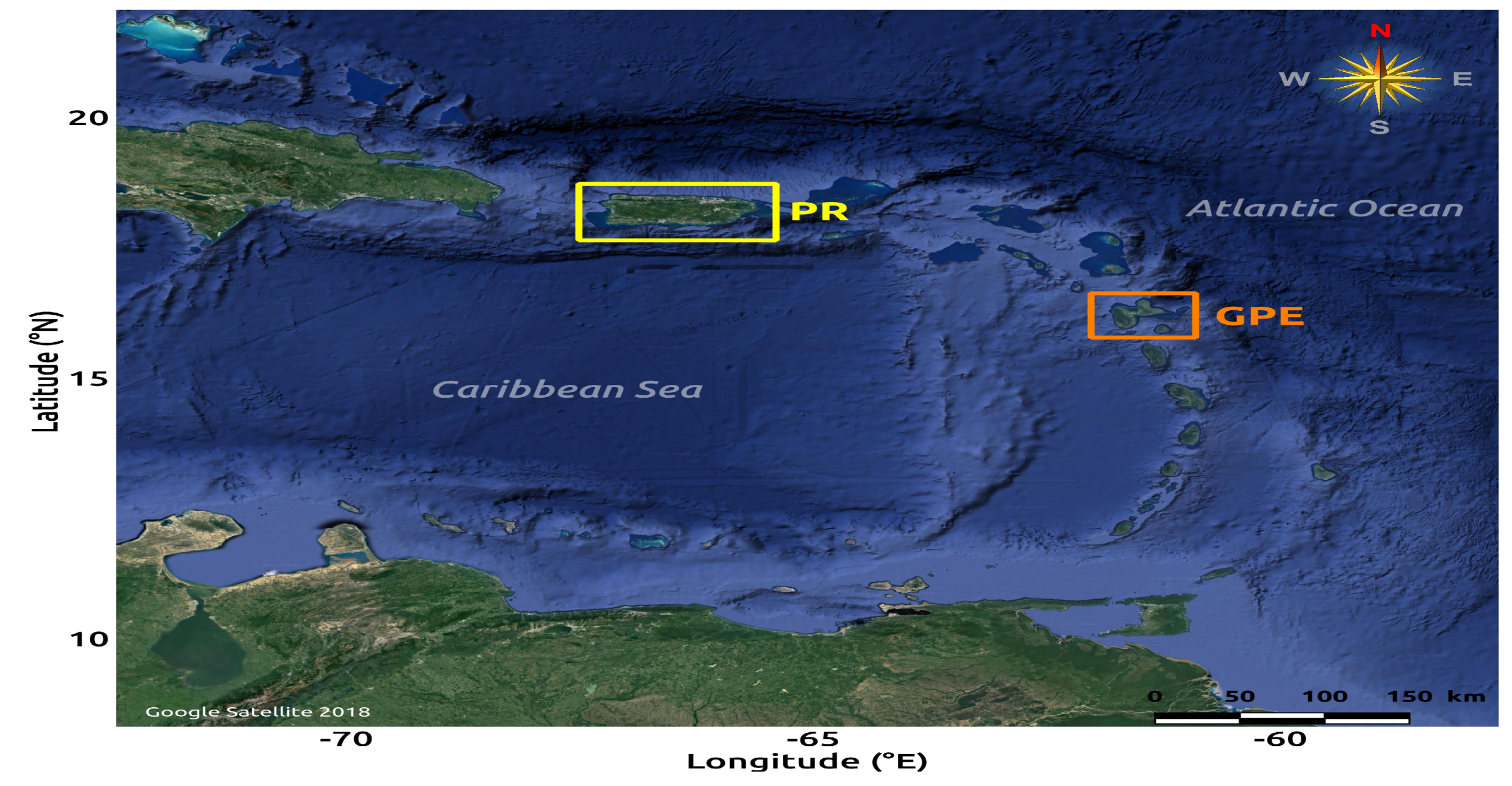
The PM10 data used come from GPE (16.242° N, −61.541° E) and PR (18.431° N, −66.142° E) whose air quality networks are Gwad’Air (http://www.gwadair.fr/; accessed on 10 February 2021) and AirNow (https://www.airnow.gov; accessed on 20 January 2021) (see Figure 1), respectively. For both networks, PM10 are collected using the Thermo Fisher Scientific Tapered Element Oscillating Microbalance (TEOM) particulate monitors 1400ab and 1400-FDMS (Filter Dynamics Measurement System) [43]. The PM10 concentrations are provided on a daily basis with an accuracy of $\pm 0.5\mathsf{\mu }$g/m${}^3$, and the reliability of these measurements is ensured by the Central Laboratory for the Monitoring of Air Quality (LCSQA) and the Environmental Protection Agency (EPA) for GPE and PR [43], respectively. Thus, two PM10 time series of 1789 and 1747 data points are available for GPE and PR from 2006 to 2010.

To carry out this study, several steps are presented: (i) the algorithms developed to compute the PM10 missing values; (ii) the choice of hypothesis tests used to verify stationarity and normality of the data; as well as autocorrelations and heteroskedasticity of the residuals from the selected model; (iii) the best model has been selected using the goodness of fit information criteria; and (iv) the forecasting performance of the coupled SARIMA-GARCH model.

2.2. Data Processing

In the PM10 database of GPE and PR, there are 37 and 79 missing values, respectively. For the correction of these missing observations, two algorithms were implemented according to the low or high dust seasons. For the low season, it is a direct imputation. To compute the missing value of PM10 located at a position i, sometimes also at $i-1$ and even at $i+1$, we took the arithmetic average of the closest data available.

So we set,

$$PM{10}_i=\frac{1}{2}\left(PM{10}_{inf}+PM{10}_{sup}\right),$$

(1)

where $PM{10}_{inf}$ is the last observed value before the missing one value, and $PM{10}_{sup}$ is the first one after.

This strategy for replacing missing observation (RMO) is suitable up to five consecutive missing values. They can be replaced by the mean value computed with Equation (1). Indeed, during the low season, PM10 concentrations have fewer fluctuations [38].

For missing values during the high season, the ratio imputation or stochastic regression method was used. This strategy aims at replacing a missing value in the data by the value predicted by a nonlinear regression model. This is due to the relationship between both PM10 variables in GPE and PR. A missing value at time t in GPE (PR) can be estimated from the value present in the PM10 data at PR (GPE) at time $t+{\delta }_t$ ($t-{\delta }_t$), where ${\delta }_t$ denotes the travel time of a particle between the two sites. Let us suppose there is $X_{P{R}_i}$ (resp. $X_{GP{E}_i}$), the observed value of PM10 in PR (resp. GPE). An estimated value $Y_{PR}^{☆}$ (resp. $Y_{GPE}^{☆}$) representing a missing observation in the PM10 dataset in PR (resp. GPE) is obtained by the following regression models:

$$\left\{\begin{array}{cc}{Y}_{P{R}_i}\left(t\right)=exp\left(\gamma +\delta ·ln\left(X_{GP{E}_i}\left(t-{\delta }_t\right)\right)\right)+u_t,& (\mathit{RMO} \mathit{in} \mathit{PM}\mathit{10}\mathit{PR} \mathit{data})\hfill \\ Y_{GP{E}_i}\left(t\right)=exp\left({\gamma }^{\prime }+{\delta }^{\prime }·ln\left(X_{P{R}_i}\left(t+{\delta }_t\right)\right)\right)+v_t,& (\mathit{RMO} \mathit{in} \mathit{PM}\mathit{10}\mathit{GPE} \mathit{data})\hfill \end{array}\right.$$

(2)

with $(\gamma ,\delta ,{\gamma }^{\prime },{\delta }^{\prime })\in {\mathbb{R}}^4,{\delta }_t\in \{1,2\};u_{t}and{v}_t$ denote numerical hazards.

Thus,

$$\left\{\begin{array}{cc}{Y}_{P{R}_i}\left(t\right)=exp\left(0.8425+0.7385·ln\left(X_{GP{E}_i}(t-1)\right)\right)+u_t,& (\mathit{RMO} \mathit{in} \mathit{PM}\mathit{10}\mathit{PR} \mathit{data})\hfill \\ Y_{GP{E}_i}\left(t\right)=exp\left(1.2733+0.6403·ln\left(X_{P{R}_i}(t+1)\right)\right)+v_t,& (\mathit{RMO} \mathit{in} \mathit{PM}\mathit{10}\mathit{GPE} \mathit{data})\hfill \end{array}\right.$$

(3)

The skewness of PM10 data in GPE and PR is approximately corrected by using the transformation method proposed by Yeo and Johnson [44], which is an improvement in the Box–Cox transformation [45,46]. The new database is constructed according to the following formula:

$$S_{i;\lambda }=\left\{\begin{array}{cc}\frac{{\left(s_i+1\right)}^{\lambda }-1}{\lambda }& si\lambda \ne 0\hfill \\ log\left(s_i\right)& si\lambda =0\hfill \end{array}\right.$$

(4)

with $S_{i;\lambda }$ (the transformed series), $s_i$ (the initial series), and $\lambda$ (the parameter of the Box–Cox transformation, $-2\le \lambda \le 2$), and i, the index or rank ranging from 1 to n, (n is the number of observations in the data set). Figure A1 shows some symmetry-related corrections made by the Box–Cox transformation.

2.3. Statistical Criterion

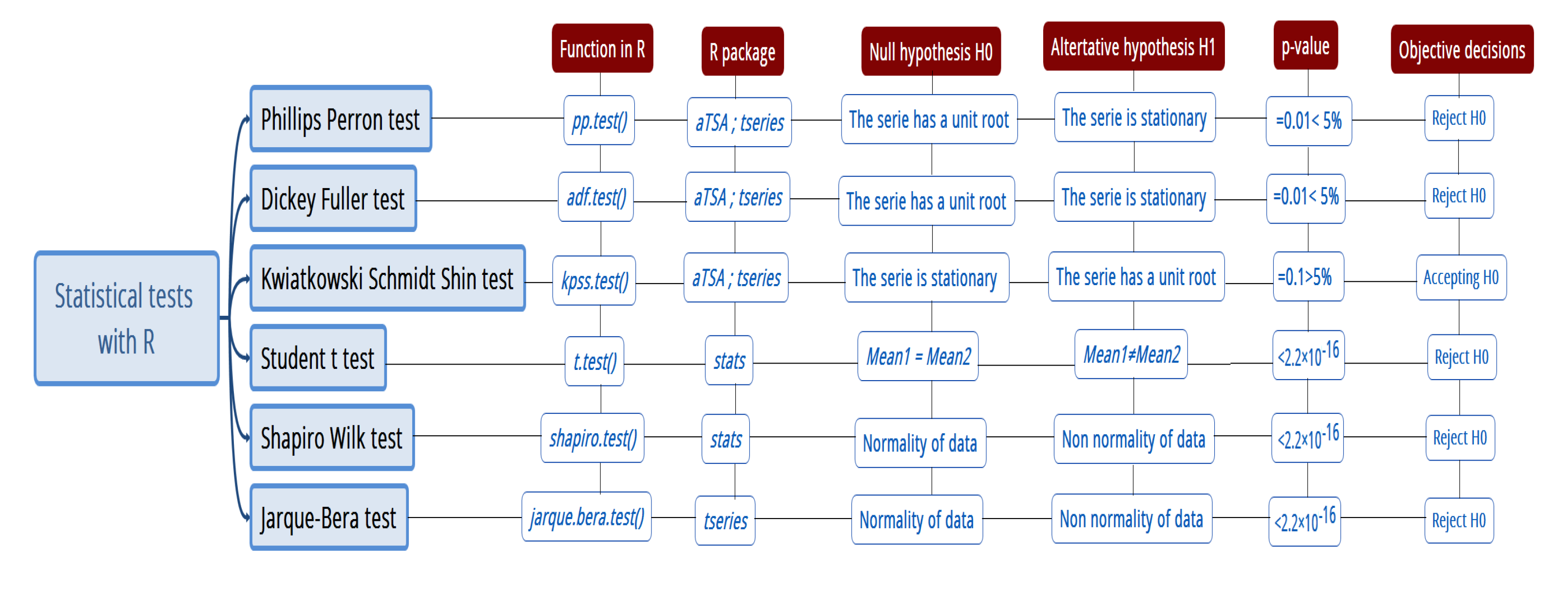
Some of the hypothesis tests in Figure A2 were used to check the stationarity and normality of the data. For stationarity, these were the Phillips Perron and Dickey Fuller tests and, for normality, the Shapiro–Wilk and Jarque–Bera tests [47,48,49]. Selection of the best stochastic model that can analyze PM10 behavior in GPE and PR is made by examining the Kullback–Leibler (K-L) information; for example, the Akaike information criterion (AIC) of the targeted model must be the smallest compared to those of the other sampled processes. Once selected, the best model is used for forecasting purposes.

2.4. SARIMA Model

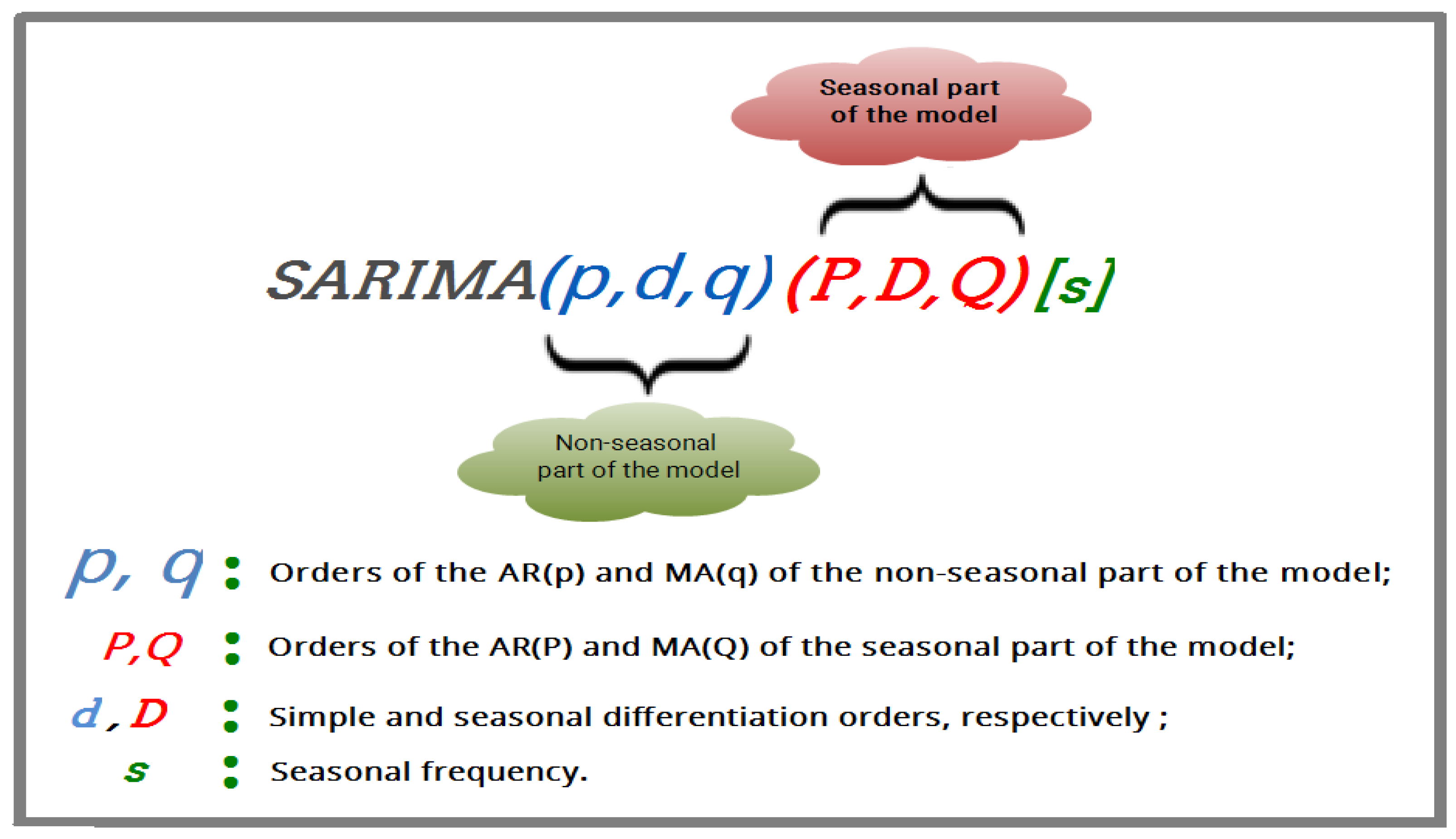
This model allows to describe the PM10 behavior according to the seasons [43]. For modeling, the orders D and d representing seasonal and non-seasonal differentiations were chosen, respectively, followed by the orders p and q of the autoregressive (AR) and moving average (MA) parts of the non-seasonal part and, finally, the orders P and Q of the AR and MA of the seasonal part of the SARIMA by looking only at the orders multiple of s, which is the periodicity of the data ($s=4$ for a quarterly series and $s=12$ for a monthly series) [50]. In the case of daily data series, we therefore took $s=365$. Figure 2 illustrates the ideas expressed.

A process $\left(X_t\right)$ follows a $SARIMA(p,d,q)(P,D,Q)\left[s\right]$ if the differentiated process $\left(Z_t\right)$ such as $Z_t={(1-B)}^d{(1-B^s)}^D{X}_t$ follows a seasonal ARMA process of the form:

$${\varphi }_p\left(B\right)\times {\mathsf{\Phi }}_P\left(B^s\right)Z_t={\theta }_q\left(B\right)\times {\mathsf{\Theta }}_Q\left(B^s\right){\zeta }_t⟺Z_t=\frac{{\theta }_q\left(B\right)\times {\mathsf{\Theta }}_Q\left(B^s\right)}{{\varphi }_p\left(B\right)\times {\mathsf{\Phi }}_P\left(B^s\right)}{\zeta }_t$$

(5)

Hence,

$${\varphi }_p\left(B\right){(1-B)}^d{\mathsf{\Phi }}_P\left(B^s\right){(1-B^s)}^D{X}_t={\theta }_q\left(B\right){\mathsf{\Theta }}_Q\left(B^s\right){\zeta }_t$$

(6)

where B is the backward operator; ${\displaystyle {\varphi }_p\left(B\right)=1-\sum _{i=1}^p{\varphi }_i{B}^i}$ and ${\displaystyle {\mathsf{\Phi }}_P\left(B^s\right)=1-\sum _{j=1}^P{\mathsf{\Phi }}_{sj}{\left(B^s\right)}^j}$ denote the polynomial functions of the autoregressive model of the non-seasonal and seasonal parts, respectively; ${\displaystyle {\theta }_q\left(B\right)=1+\sum _{k=1}^q{\theta }_k{B}^k}$ and ${\displaystyle {\mathsf{\Theta }}_Q\left(B^s\right)=1+\sum _{l=1}^Q{\mathsf{\Theta }}_{sl}{\left(B^s\right)}^l}$ denote the polynomial functions of $MA\left(q\right)$ and $MA\left(Q\right)$ of the non-seasonal and seasonal parts, respectively; ${\zeta }_t$ is the residuals of the SARIMA model [51,52].

For the choice of the orders $p,q,P,and Q$, the auto.arima function of was used. This function uses a variant of the Hyndman–Khandakar algorithm, which combines unit root tests, $AI{C}_c$ minimization, and the maximum likelihood estimator (MLE) to obtain an ARIMA model [53]. The orders d and D were obtained from the stationarity and periodicity criteria applied to the data series.

2.5. GARCH Model

Concerning the residuals of the SARIMA model, we investigated their autocorrelations using the McLeod–Li test. Engle’s test allows us to evaluate their GARCH character, i.e., their conditional heteroskedasticity.

A process ${\zeta }_t$ follows a semi-strong $GARCH(\alpha ,\beta )$ process if:

$${\displaystyle \forall t\in {\mathbb{Z}}^{☆},E\left({\zeta }_t/{\mathcal{F}}_{t-1}\right)=0and{\sigma }_t^2=V\left({\zeta }_t/{\mathcal{F}}_{t-1}\right)=\omega +\sum _{i=1}^{\alpha }{a}_i{\zeta }_{t-i}^2+\sum _{j=1}^{\beta }{b}_j{\sigma }_{t-j}^2.}$$

(7)

${\zeta }_t$ follows a strong $GARCH(\alpha ,\beta )$ process if:

$${\displaystyle \forall t\in {\mathbb{Z}}^{☆},{\zeta }_t={\sigma }_t{Z}_t,and{\sigma }_t^2=V\left({\zeta }_t/{\mathcal{F}}_{t-1}\right)=\omega +\sum _{i=1}^{\alpha }{a}_i{\zeta }_{t-i}^2+\sum _{j=1}^{\beta }{b}_j{\sigma }_{t-j}^2,}$$

(8)

where,

• $\omega ,a_i(i=1,2,\dots ,\alpha ),b_j(j=1,2,\dots ,\beta )$ some constants [54,55];
• ${\mathcal{F}}_{t-1}$ denotes a filtering of all information of the process ${\zeta }_t$ until the time $t-1$;
• $Z_t\sim i.i.d.WN(0,1)$;
• for any time $t,{\sigma }_t^2$ denotes the conditional variance as a function of ${\zeta }_t^2$, which we are trying to simulate.

The $GARCH(\alpha ,\beta )$ model admits a second-order stationary solution if:

$${\displaystyle \sum _{i=1}^{\alpha }{a}_i+\sum _{j=1}^{\beta }{b}_j<1.}$$

(9)

In this case, unconditional variance, i.e. marginal variance of the $GARCH(\alpha ,\beta )$ process as a function of its parameters, is defined as:

$$V\left({\zeta }_t\right)=E\left({\zeta }_t^2\right)=\frac{\omega }{{\displaystyle 1-\left(\sum _{i=1}^{\alpha }{a}_i+\sum _{j=1}^{\beta }{b}_j\right)}}.$$

(10)

To find the GARCH model fitted to the residuals of the SARIMA model, we considered the time series defined by the square of the residuals, arguing

$$\left({\zeta }_t\right)\sim GARCH(\alpha ,\beta )⟹\left({\zeta }_t^2\right)\sim ARMA\left(max(\alpha ,\beta ),\beta \right).$$

(11)

In practice, the $\alpha$ and $\beta$ orders of the $GARCH(\alpha ,\beta )$ model are such that both $\alpha$ and $\beta$ do not exceed 1 or 2 [55].

Thus, a coupled SARIMA-GARCH model was considered in this study.

2.6. Indexes of Forecast Evaluation

The forecast evaluation indexes used were the Mean Absolute Percentage Error (MAPE), the Mean Absolute Scaled Error (MASE), and the U statistic of Theil. We denote $e_t$, the prediction error at a time t. It is the difference between the measured value $y_t$ and the predicted value ${\tilde{y}}_t$ at time t. Let us consider a validation period with n elements, $t=1,2,\dots ,n$. The performance measures of the forecast are defined below:

The MAPE gives the percentage of the difference (on average) between the forecast and the observed value [56]. It is defined as follows:

$$MAPE=\frac{1}{n}\sum _{t=1}^n\left|\frac{e_t}{y_t}\right|\times 100,$$

(12)

where $e_t=y_t-{\tilde{y}}_t$.

The scale for MAPE has been stated by Lewis [57]: $MAPE\le 10\%$ (highly effective forecast); $10\%<MAPE\le 20\%$ (good forecast); $20\%<MAPE\le 50\%$ (reasonable forecast); $MAPE>50\%$ (ineffective forecast).

For negative or values close to zero, MASE is more appropriate than MAPE [58]. The MASE is computed by the following equation:

$$MASE=\underset{1\le t\le n}{mean}\left(\right|q_t\left|\right)and{q}_t=\frac{e_t}{{\displaystyle \frac{1}{n-s}\sum _{j=s+1}^n|y_j-y_{j-s}|}},$$

(13)

with $y_{j-s}={\tilde{y}}_j$ and s is the seasonal period.

When $MASE<1$, the errors of the prediction model are smaller than the one-step errors of the naive method [58].

The U statistic is an approach developed by Theil [59,60]. This accuracy measure allows a relative comparison between formal forecasting methods and naive methods. The U statistic of Theil is defined by two formulas:

$$U_1=\frac{\sqrt{{\displaystyle \frac{1}{n}\sum _{t=1}^n{e}_t^2}}}{\sqrt{{\displaystyle \frac{1}{n}\sum _{t=1}^n{y}_t^2}}+\sqrt{{\displaystyle \frac{1}{n}\sum _{t=1}^n{\tilde{y}}_t^2}}}and{U}_2=\sqrt{\frac{{\displaystyle \sum _{t=1}^{n-1}{\left(\frac{e_t}{y_{t-1}}\right)}^2}}{{\displaystyle \sum _{t=1}^{n-1}{\left(\frac{y_t-y_{t-1}}{y_{t-1}}\right)}^2}}},$$

(14)

with $0\le U_1\le 1$ and $U_2\ge 0$.

There is greater accuracy in the forecasts when Theil’s $U_1$ statistic is close to 0. The measurement scale for $U_2$ is as follows: if $U_2=1$, the naive method is as good as the forecasting model evaluated; if $U_2<1$, the forecasting model used is better than the naive method; if $U_2>1$, the naive method performs better than the forecasting model [61].

3. Results and Discussion

3.1. PM10 Descriptive Statistics

Before focusing on the temporal dynamics of PM10 data in GPE and PR, we firstly review their statistical properties before and after correction of missing observations in order to have a clearer understanding of their behavior.

According to the information in

Table 1. Some statistics of PM10 data in GPE and PR from 2006 to 2010.

Statistics	Before Correction		After Correction
	$\underset{(\mathbf{n}=\mathbf{1789})}{\mathbf{PM}\mathbf{10}\mathbf{GPE}}$	$\underset{(\mathbf{n}=\mathbf{1747})}{\mathbf{PM}\mathbf{10}\mathbf{PR}}$	$\underset{(\mathbf{n}=\mathbf{1826})}{\mathbf{PM}\mathbf{10}\mathbf{GPE}}$	$\underset{(\mathbf{n}=\mathbf{1826})}{\mathbf{PM}\mathbf{10}\mathbf{PR}}$
Minimum	$4.00$	$7.00$	$4.00$	$7.00$
First quartile	$17.00$	$17.00$	$17.00$	$17.00$
Median	$21.00$	$21.00$	$21.00$	$21.00$
Mean	$26.59$	$25.54$	$26.62$	$25.65$
Third quartile	$30.00$	$27.00$	$30.00$	$28.00$
Maximum	$164.00$	$197.00$	$164.00$	$197.00$
Missing data	$37.00$	$79.00$	−	−
Variance	$271.46$	$263.52$	$266.94$	$258.13$
Standard deviation	$16.48$	$16.23$	$16.34$	$16.07$
Coefficient of variation	$0.62$	$0.64$	$0.61$	$0.63$
Skewness	$2.69$	$3.61$	$2.69$	$3.57$
Kurtosis	$10.81$	$19.78$	$10.97$	$19.67$

, the minimum, maximum, first, and second quartiles (median) computed in each data set remain the same before and after data correction. Some other statistics such as indicators of dispersion (variance, standard deviation, and coefficient of variation) and shape measures (skewness and kurtosis) were almost identical. This similarity validates the implemented algorithms defined in Section 2.2.

The skewness coefficients in GPE and PR were different from 0, which is the reference value for the normality of a process [62,63]. Thus, the PM10 distribution for each area is not symmetric. Estimated kurtosis coefficients of 10.97 and 19.67 in GPE and PR exhibited a leptokurtic distribution.

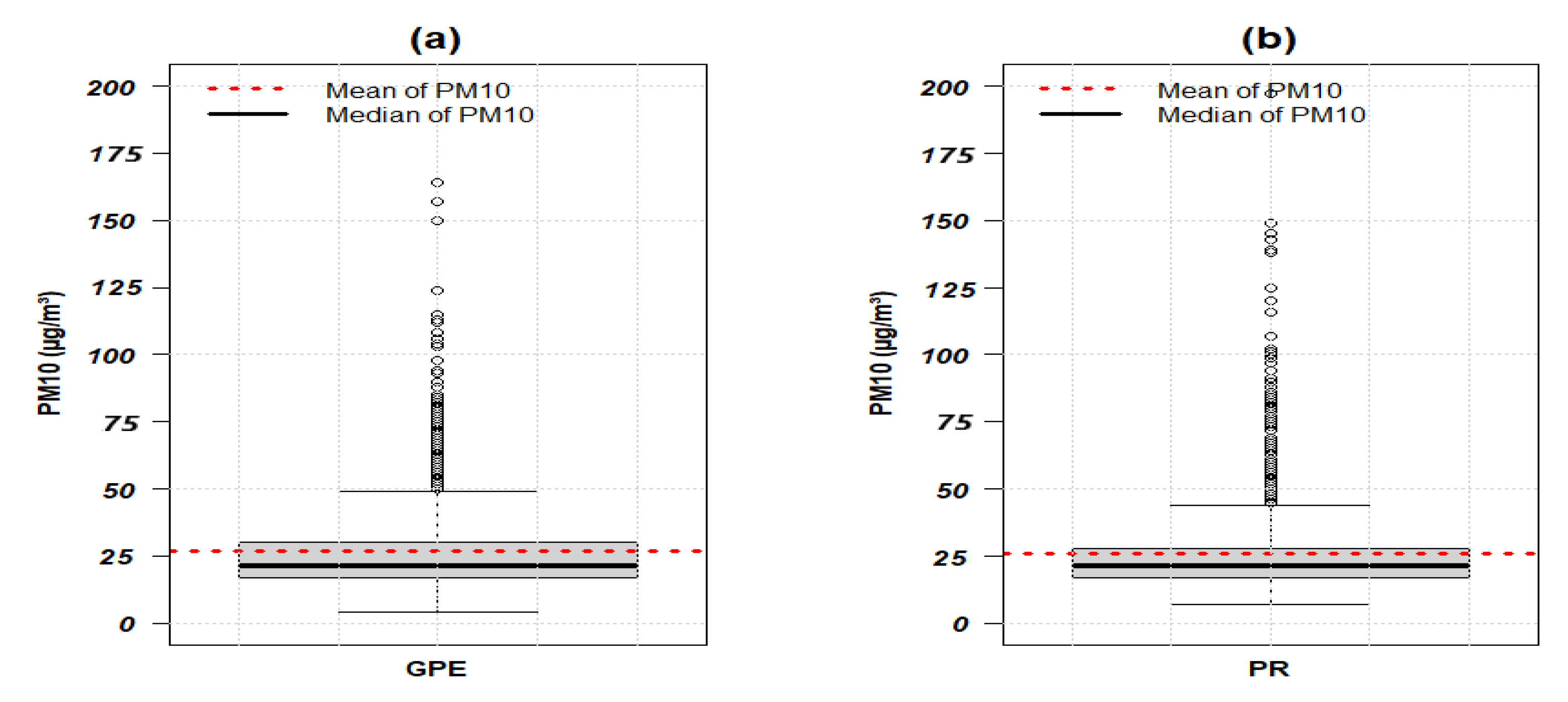
Boxplots in Figure 3 illustrate the extreme values (values greater than the median value plus twice the interquartile range) observed in the PM10 database of GPE (10.02%) and PR (9.75%). These values can be due to sand haze, fires, or volcanic eruptions [64]. Thus, the same extreme event seems to have an impact on both islands. It involves a sudden and instantaneous increase in particulate pollution, called a PM10 jump. These jumps can be modeled by stochastic differential equations that take into account the dynamics of space, time, and randomness [65].

The red curve in the scatterplot in Figure 4 represents the second-order polynomial regression. For $min\left(PM10\right)\le PM10GPE\left(PM10PR\right)\le 50\mathsf{\mu }$g/m${}^3$, there is a homogeneity in the points distribution. For the other points, i.e., $PM10\ge 50\mathsf{\mu }$g/m${}^3$, the distribution is heterogeneous. Thus, most of the data were below the $50\mathsf{\mu }$g/m${}^3$ threshold recommended by the World Health Organization (WHO) [66]. These results are in agreement with the relationship stated in Section 2.2. The quadratic regression model equation where PM10PR (PM10GPE) is the response variable, and $PM10GPE\left(PM10PR\right)$ the explicative variable, is given by Equations (15) and (16), respectively:

$$PM10PR=7.2143+0.7502\left(PM10GPE\right)-0.0016{\left(PM10GPE\right)}^2+{\xi }_1,$$

(15)

$$PM10GPE=5.0056+0.9537\left(PM10PR\right)-0.0031{\left(PM10PR\right)}^2+{\xi }_2,$$

(16)

where ${\xi }_1$ and ${\xi }_2$ are the residual values.

The regression results show a p-value < 2.2 × 10⁻¹⁶. The coefficient of determination $R^2$ in the first case was 37.19%; this indicates that 37.19% of the variation in the dependent variable was represented by the model. The Spearman’s correlation coefficient $\rho$ was 0.5084, i.e., 50.84%: there is therefore a positive relationship of average intensity between PM10GPE and PM10PR variables. In the second case, we have $R^2=38.94\%$ and $\rho =50.84\%$. These percentages prove once again that when a large-scale event occurs in GPE, it is felt at PR.

The results in

Table 2. The results of the quadratic regression model.

Regression	Coefficients	Estimate	Std. Error	t Value	Pr(>|t|)
1	Intercept	$7.2143$	$0.9453$	$7.63$	3.71 × 10−14
	PM10GPE	$0.7502$	$0.0490$	$15.32$	<2.00 × 10−16
	$I\left(PM10GP{E}^2\right)$	$-0.0016$	$0.0005$	$-3.38$	$7.36$ × 10−4
2	Intercept	$5.0056$	$0.9183$	$5.45$	$5.69$× 10−8
	PM10PR	$0.9537$	$0.0461$	$20.71$	<2.00 × 10−16
	$I\left(PM10P{R}^2\right)$	$-0.0031$	$0.0004$	$-7.99$	$2.29$ × 10−15

show that the coefficients of both regression models in Equations (15) and (16) are statistically significant (p-value $<5\%$). With the significance of the quadratic term, the curvature trend of the scatterplot in Figure 4 is approved. Thus, second-order polynomial regression provides the model that fits the raw data.

3.2. Chronogram and Decomposition of PM10 Data

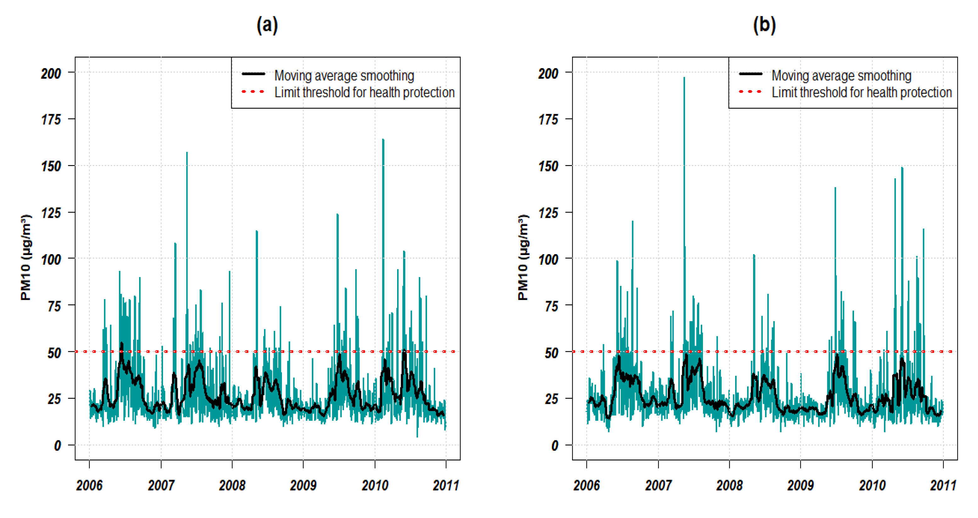
Figure 5 illustrates the temporal variations of PM10 concentration at GPE and PR. The main PM10 daily concentrations range from 0 to the mean value of each distribution, which is approximately $26\mathsf{\mu }$g/m${}^3$. During the high dust season, we can observe that PM10 values frequently exceed the $50\mathsf{\mu }$g/m${}^3$ recommended by the WHO [66].

A non-parametric filtering method was used in Figure 5; it is the moving average smoothing whose aim is to approach the trend by attenuating irregular fluctuations. The average evolves in periods of about $p=24$ h. This method also allows us to detect the time of the trend reversal; we obtained a picture of the daily and seasonal average dynamics of the Saharan dust cloud. A trivial analysis of Figure 5 shows that the main highest PM10 peaks are observed during the high dust season in summer due to dust outbreaks as shown by PR in May 2007. However, extreme events such as volcanic eruptions can also lead to a sharp increase in PM10 concentrations during the low dust season. This is the case in GPE with the eruption of Soufrière on Montserrat in February 2010 [67].

Figure 6 presents the decomposition of the two PM10 data series in GPE and PR according to an additive scheme. The top graph in (a) and (b) of it can be seen as a sum of:

−

a trend that is the average behavior of the two data series, i.e., their evolution over the long term. This trend is characterized by a linear increase or decrease at irregular intervals. Each time process shows a monotonic behavior from one year to another;

−

a seasonal component (cycle) that corresponds to different cases where PM10 phenomenon repeats at regular or periodic intervals. Here, the period is intra-year; strong pollution peaks are observed in the middle of each year;

−

a random component or noise or residual. This corresponds to low-intensity fluctuations of a stochastic nature and is part of the disturbing elements [50].

Intuitively and based on PM10 studies in the Caribbean area [68,69,70,71], we assumed that this decomposition represents for the stochastic process $X_t$ the sum of the background atmosphere ($B_t$ = anthropogenic activities + marine aerosol), African dust seasonality ($S_t$ = mineral dust), and extreme events processes ($C_t$). The $B_t$ and $S_t$ terms will be modeled by the SARIMA process. The extreme events, noted $C_t$, will be described by the GARCH model.

Overall, one can notice that the decompositions in Figure 6 seem to follow the same temporal pattern for both islands. PM10 average concentrations are the lowest in 2009, while they are higher in 2007 and 2010 in PR and GPE for the reasons aforementioned.

3.3. Analysis of Seasonal Effects

The decomposition method plotted in Figure 6 shows a strong seasonal component in the PM10 data in GPE and PR. The autocorrelation function represented in Figure 7 also illustrates the existence of this seasonality. The vertical lines, with equations $v=365n,n\in \{1,2,3,4,5\}$, represent offsets that are multiples of 365. They are thus retrogrations of the seasonal period.

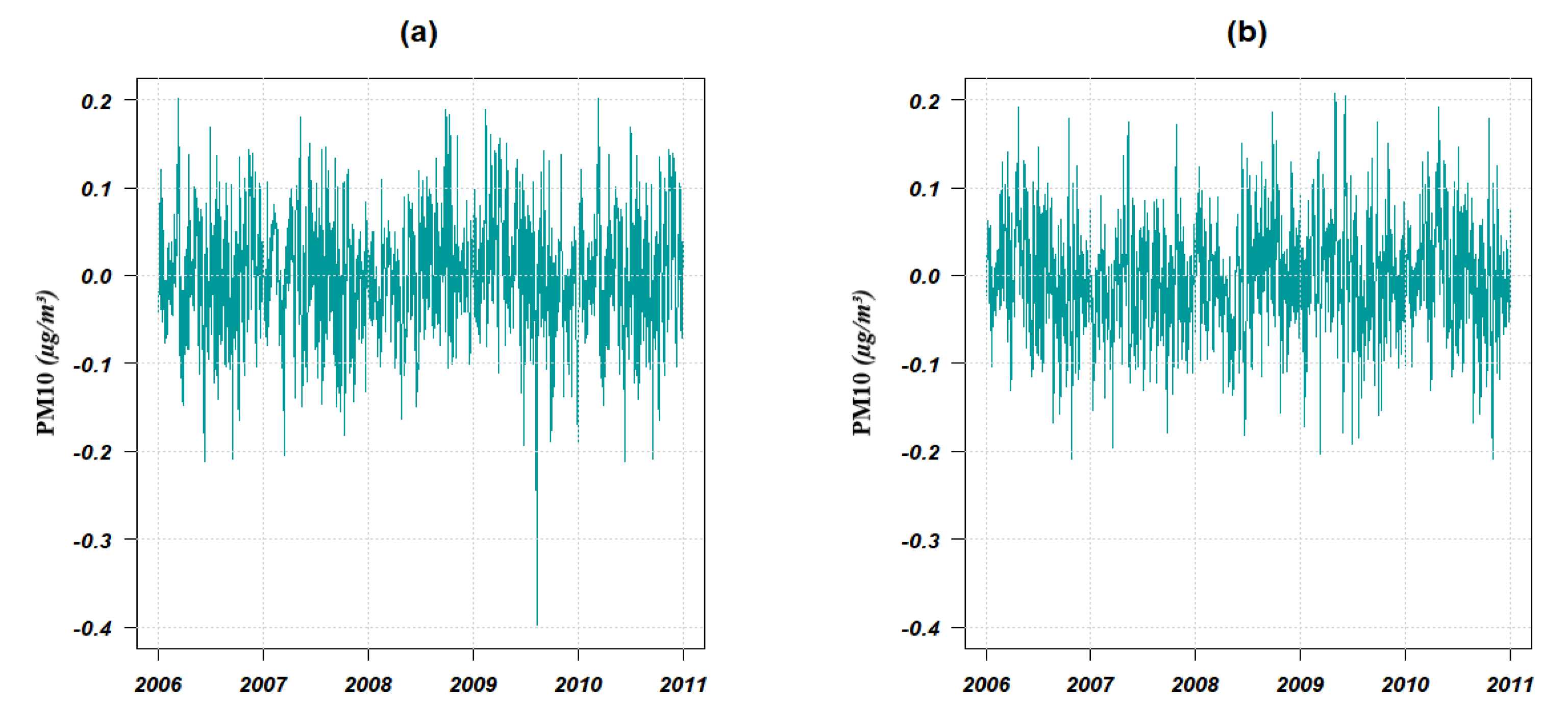
To build the model, the differentiated series modeling was firstly performed. As the original data series is stationary but exhibits seasonality, we chose a seasonal differentiation before choosing the appropriate orders for our process. Yeo and Johnson’s formula in (4), which is derived from the Box–Cox transformation, was applied to solve some data skewness problems. Figure 8 represents the PM10 time series obtained after the Box–Cox transformation and differentiation. Although transformed, some lags were observed in both PM10 time series.

3.4. Selection of the PM10 Model

Table 3. Checking of the PM10 model information criteria in GPE and PR.

PM10GPE		PM10PR
Model	AIC	Model	AIC
$SARIMA(3,0,1)(0,1,0)\left[365\right]$	$-2964.79$	$SARIMA(1,0,1)(0,1,0)\left[365\right]$	$-3112.59$
$SARIMA(2,0,1)(0,1,0)\left[365\right]$	$-2961.21$	$SARIMA(2,0,1)(0,1,0)\left[365\right]$	$-3108.94$
$SARIMA(4,0,2)(0,1,0)\left[365\right]$	$-2961.61$	$SARIMA(0,0,1)(0,1,0)\left[365\right]$	$-3005.81$
$SARIMA(2,0,0)(0,1,0)\left[365\right]$	$-2960.96$	$SARIMA(1,0,2)(0,1,0)\left[365\right]$	$-3109.79$
$SARIMA(1,0,3)(0,1,0)\left[365\right]$	−2965.30	$SARIMA(0,0,5)(0,1,0)\left[365\right]$	−3114.69

shows goodness of fit and the selection of the two $SARIMA(1,0,3)(0,1,0)\left[365\right]$ and $SARIMA(0,0,5)(0,1,0)\left[365\right]$ processes as models with the smallest AIC intended to explain the behavior of PM10 data in GPE and PR from 2006 to 2010, respectively.

Student’s t test for significance of the model parameters constructed allows to reject the $H_0$ hypothesis corresponding to nullity coefficients. The latter are therefore significant.

Table 4. Estimation and significance of PM10 model parameters in GPE and PR; C.I.: Confidence Interval.

Model	Parameters	Estimate	Std. Error	t-Test	p-Value	Coefficient C.I.
						2.5%	97.5%
$SARIMA(1,0,3)(0,1,0)\left[365\right]$	$AR1$	$0.8275$	$0.0933$	$8.87$	$0.000000$	$0.6446$	$1.0104$
	$MA1$	$-0.2186$	$0.0989$	$-2.21$	$0.027081$	$-0.4124$	$-0.0248$
	$MA2$	$-0.2338$	$0.0698$	$-3.35$	$0.000811$	$-0.0970$	$-0.0970$
	$MA3$	$-0.0931$	$0.0463$	$-2.01$	$0.044123$	$-0.0024$	$-0.0024$
$SARIMA(0,0,5)(0,1,0)\left[365\right]$	$MA1$	$0.5947$	$0.0261$	$22.75$	$0.000000$	$0.5435$	$0.6460$
	$MA2$	$0.2878$	$0.0304$	$9.46$	$0.000000$	$0.2282$	$0.3474$
	$MA3$	$0.1457$	$0.0313$	$4.66$	$0.000003$	$0.0844$	$0.2069$
	$MA4$	$0.1112$	$0.0295$	$3.77$	$0.000161$	$0.0534$	$0.1689$
	$MA5$	$0.0959$	$0.0259$	$3.70$	$0.000216$	$0.0451$	$0.1468$

shows that this criterion was validated (p-value $<5\%$). Moreover, the t-test equivalent to the quotient of each coefficient divided by the standardized error is greater than 1.96 in absolute value.

• The expression of the stochastic process $\left(X_t\right)$ describing PM10 in GPE and following a $SARIMA(1,0,3)(0,1,0)\left[365\right]$ is written:

  $$(1-0.8275B)(1-B^{365})X_t=(1-0.2186B-0.2338B^2-0.0931B^3){\zeta }_t$$

  (17)
  Equivalently,

  $$X_t=0.8275X_{t-1}+X_{t-365}-0.8275X_{t-366}-0.2186{\zeta }_{t-1}-0.2338{\zeta }_{t-2}-0.0931{\zeta }_{t-3}+{\zeta }_t$$

  (18)

  with ${\zeta }_t\sim WN(0;0.0875)$ and B, the backward operator.
• The background sources of the PM10 at PR can be described by the stochastic process $\left(Y_t\right)$ following a $SARIMA(0,0,5)(0,1,0)\left[365\right]$. The mathematical expression of $Y_t$ is then written:

  $$\begin{gathered} (1-B^{365})Y_t=(1+0.5947B+0.2878B^2+0.1457B^3+0.1112B^4+0.0959B^5){ϵ}_t \\ \Updownarrow \end{gathered}$$

  (19)

  $$Y_t=Y_{t-365}+0.5947{ϵ}_{t-1}+0.2878{ϵ}_{t-2}+0.1457{ϵ}_{t-3}+0.1112{ϵ}_{t-4}+0.0959{ϵ}_{t-5}+{ϵ}_t$$

  (20)

  with ${ϵ}_t\sim WN(0;0.08313)$ and B, the backward operator.

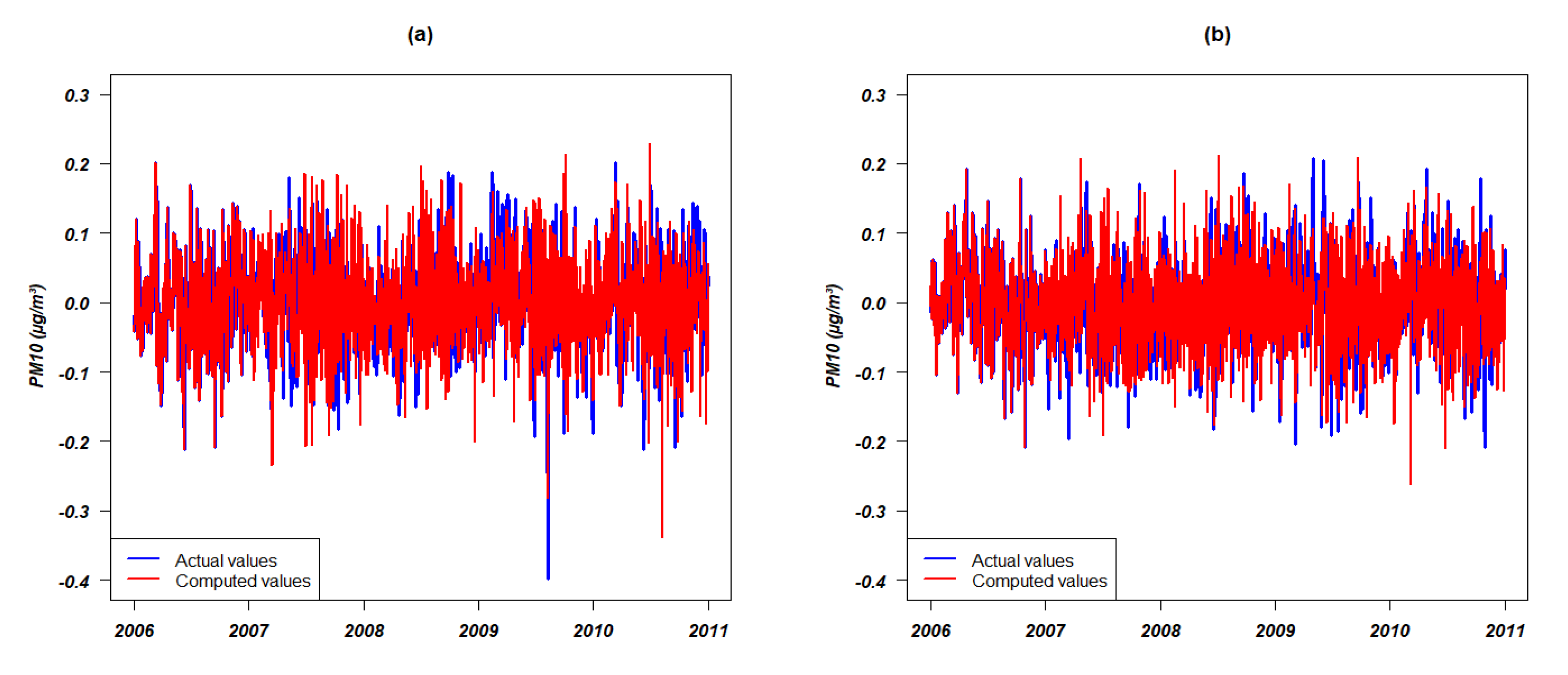
Figure 9 and Figure A3 serve as a comparison between the actual transformed series data and the computed values of the SARIMA model. A slight discrepancy can be observed between these two quantities. This bias may be due to the mathematical transformations used on the empirical data such as the Box-Cox transformation for example.

3.5. Stationarity of Each PM10 Model

The process $\left(X_t\right)$ is stationary if the zeros of polynomials ${\varphi }_p\left(x\right)=1-0.8275x$ and ${\theta }_q\left(x\right)=1-0.2186x-0.2338x^2-0.0931x^3$ ($p=1$ and $q=3$) have moduli exceeding 1 or if the roots of each equation ${\varphi }_1\left(x\right)=0$ and ${\theta }_3\left(x\right)=0$ are outside the unit circle. So we have:

$${\varphi }_1\left(x\right)=0⟺x\in \left\{1.21\right\}$$

(21)

$${\theta }_3\left(x\right)=0⟺x\in \{1.9914308147i-1.9506390977;-1.9914308147i-1.9506390977;1.39\}$$

(22)

Similarly, the process $\left(Y_t\right)$ is stationary if zeros of polynomial ${\theta }_q$ such that ${\theta }_q\left(y\right)=1+0.5947y+0.2878y^2+0.1457y^3+0.1112y^4+0.0959y^5$ ($q=5$) have moduli exceeding 1 or if the roots of equation ${\theta }_5\left(y\right)=0$ are outside the unit circle.

$$\begin{array}{c}\hfill {\theta }_5\left(y\right)=0⟺y\in \{0.9789451206+1.356173123i;0.9789451206-1.356173123i;\end{array}$$

$$\begin{array}{c}\hfill -0.7807991779+1.336453025i;-0.7807991779-1.336453025i;-1.555833074\}\end{array}$$

(23)

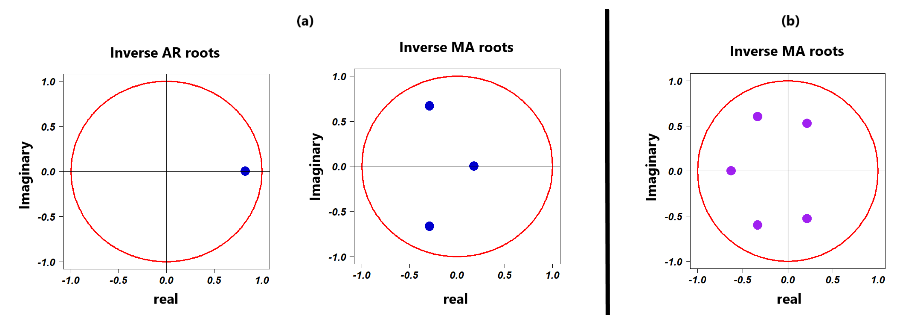
The non-seasonal first-order autoregressive function ${\varphi }_1$ and third-order moving average function ${\theta }_3$ of the PM10 model in GPE, as well as the moving average function ${\theta }_5$ from PM10 at PR admit zeros with the modulus of each exceeding 1. Stationarity conditions for constructed models require that the complex zeros of each function ${\varphi }_1,{\theta }_3,{\theta }_5$ must be outside the unit circle. Equivalently, their inverse is inside the unit circle as illustrated in Figure 10 [53].

3.6. Dynamics of Conditional Heteroskedasticity of the Residuals from the SARIMA Model

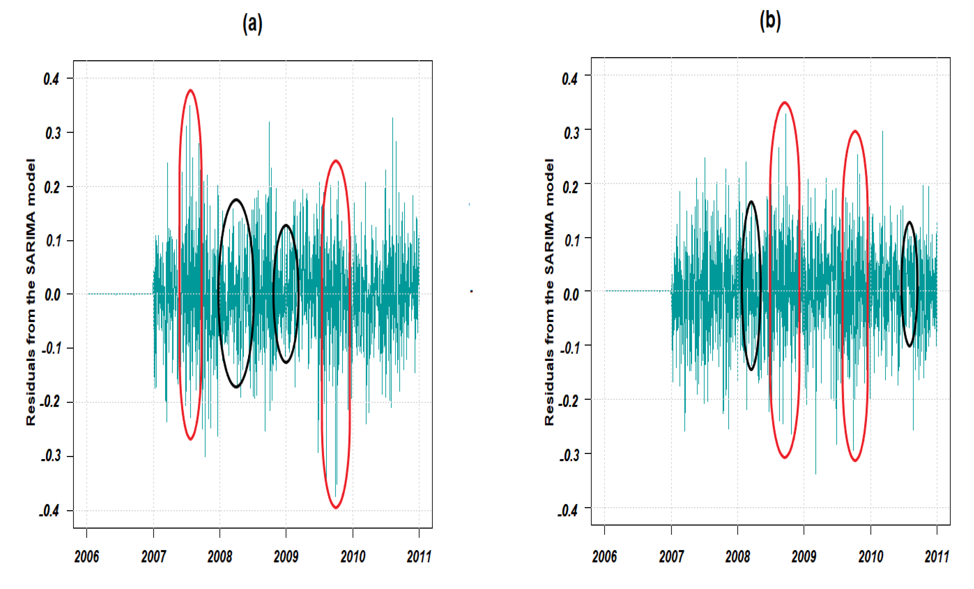
Visual evidence of the GARCH effect for residuals from the SARIMA model is illustrated in Figure 11. In fact, we observed locations of high and low variability. This clustering is noticeable in Figure 12 of the squared residuals.

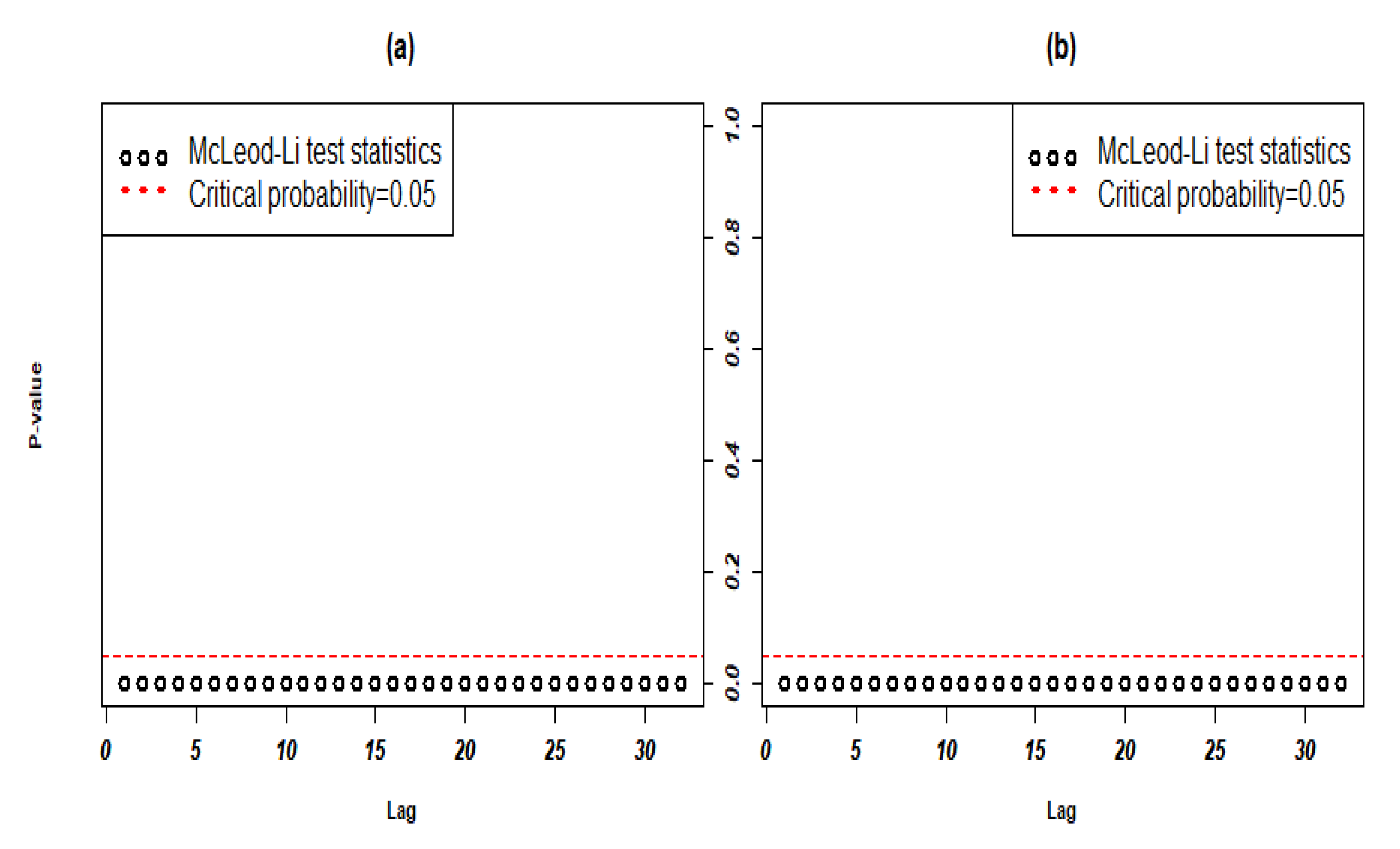
The results of the McLeod–Li autocorrelation test in Figure 13 and Arch Engle test in

Table 5. Normality, autocorrelation, and heteroskedasticity tests of residuals from the SARIMA model.

	PM10GPE			PM10PR
Hypothesis Tests	Statistics	Df	p-Value	Statistics	Df	p-Value
Shapiro–Wilk	$0.97$	NA	<2.2 $\times {10}^{-16}$	$0.97$	NA	<2.2 $\times {10}^{-16}$
Jarque–Bera	$302.24$	2	<2.2 $\times {10}^{-16}$	$175.77$	2	<2.2 $\times {10}^{-16}$
ARCH LM-test	$175.46$	20	<2.2 $\times {10}^{-16}$	$114.48$	20	<3.0 $\times {10}^{-15}$

NA : Not Available.

allow to confirm the residual variability indicated in Figure 11 and Figure 12. Thus, residual errors of both PM10 models in GPE and PR exhibit a GARCH effect and are therefore auto-correlated. Some extreme events may involve these shocks in PM10 data for both islands.

The null hypothesis $H_0$ of homoskedasticity between residuals from the SARIMA was rejected because the p-value of the McLeod–Li test was less than 5%. Therefore, the alternative hypothesis $H_1$ of heteroskedasticity was accepted. Shapiro–Wilk and Jarque Bera normality tests in Table 5 with p-values less than 5% show that residuals in the PM10 model do not follow a normal distribution. Figure 14 is a visual representation of this. It is called a long-tailed distribution in the literature.

Contrary to other studies [24,30,32], our results showed that the residuals of the SARIMA model do not follow a normal distribution (see Figure 14). This demonstrates the special feature of PM10 fluctuations in GPE and PR. Consequently, the residual part of the SARIMA model has been investigated by a GARCH model.

Some non-linear models related to the GARCH process are presented in

Table 6. Residual model information criteria for the PM10 $SARIMA$ process in GPE and PR.

PM10GPE		PM10PR
Model	AIC	Model	AIC
$GARCH(1,0)$	$-2.3038$	$GARCH(1,0)$	$-2.4006$
$GARCH(1,1)$	−3.3754	$GARCH(1,1)$	−3.8294
$GARCH(2,0)$	$-2.3381$	$GARCH(2,0)$	$-1.1025$
$GARCH(2,1)$	$-3.3716$	$GARCH(2,1)$	$-3.8223$
$GARCH(2,2)$	$-3.3714$	$GARCH(2,2)$	$-3.8229$
$GARCH(3,0)$	$-2.7294$	$GARCH(3,0)$	$-3.0561$
$GARCH(3,1)$	$-3.3710$	$GARCH(3,1)$	$-3.8239$
$GARCH(3,2)$	$-3.3698$	$GARCH(3,2)$	$-3.8255$

. By using the Akaïke information criterion (AIC), we are able to choose the best of them, i.e., the one with the smallest AIC. This process allows us to describe the heteroskedasticity of the residuals of the SARIMA model. In the stochastic process $X_t$, the GARCH model is applied to the $C_t$ term component (extreme events process).

Finally, the residuals from each of the PM10 models in GPE and PR follow a GARCH(1,1) process. The coefficients of this non-linear model are shown in

Table 7. Residual model parameters from the $SARIMA$ process for PM10 at GPE and PR.

	PM10GPE				PM10PR
Parameters	Estimate	Std. Error	t Value	Pr(>|t|)	Estimate	Std. Error	t Value	Pr(>|t|)
$\omega$	8.652 $\times {10}^{-7}$	$0.000000$	$2.18$	$0.029506$	8.567 $\times {10}^{-8}$	$0.000001$	$0.06$	$0.94943$
$a_1$	1.622 $\times {10}^{-1}$	$0.009482$	$17.10$	$0.000000$	1.951 $\times {10}^{-1}$	$0.009912$	$19.68$	$0.00000$
$b_1$	8.368 $\times {10}^{-1}$	$0.008301$	$100.81$	$0.000000$	8.039 $\times {10}^{-1}$	$0.008671$	$92.71$	$0.00000$

.

The expression of each of the residual models from the SARIMA process of PM10 in GPE and PR is given by Equations (24) and (25), respectively.

$$\left\{\begin{array}{c}{\zeta }_t={\sigma }_t{Z}_t,Z_t\sim WN(0,1)\hfill \\ {\sigma }_t^2=8.652e-07+0.1622{\zeta }_{t-1}^2+0.8368{\sigma }_{t-1}^2\hfill \end{array}\right.$$

(24)

$$\left\{\begin{array}{c}{\zeta }_t^{\prime }={\sigma }_t^{\prime }{Z}_t,Z_t\sim WN(0,1)\hfill \\ {{\sigma }_t^{\prime }}^2=8.567e-08+0.1951{\left({\zeta }_{t-1}^{\prime }\right)}^2+0.8039{\left({\sigma }_{t-1}^{\prime }\right)}^2\hfill \end{array}\right.$$

(25)

The GARCH processes built from the residuals of the PM10 SARIMA model in GPE or PR and defined in the Equations (24) and (25) are stationary as the persistence of the variability represented by the sum of the coefficients $a_1$ and $b_1$ is less than 1. The coefficients $\omega$ that are included are $8.652\times {10}^{-7}$ and $8.567\times {10}^{-8}$, respectively . They represent the lower boundary below which the variability of PM10 values cannot cross. The $a_1$ coefficients 0.1622 and 0.1951 denote the effect of extreme events on the PM10 distribution at GPE and PR. On the other hand, the $b_1$ coefficients 0.8368 and 0.8039 indicate the persistence of the phenomenon.

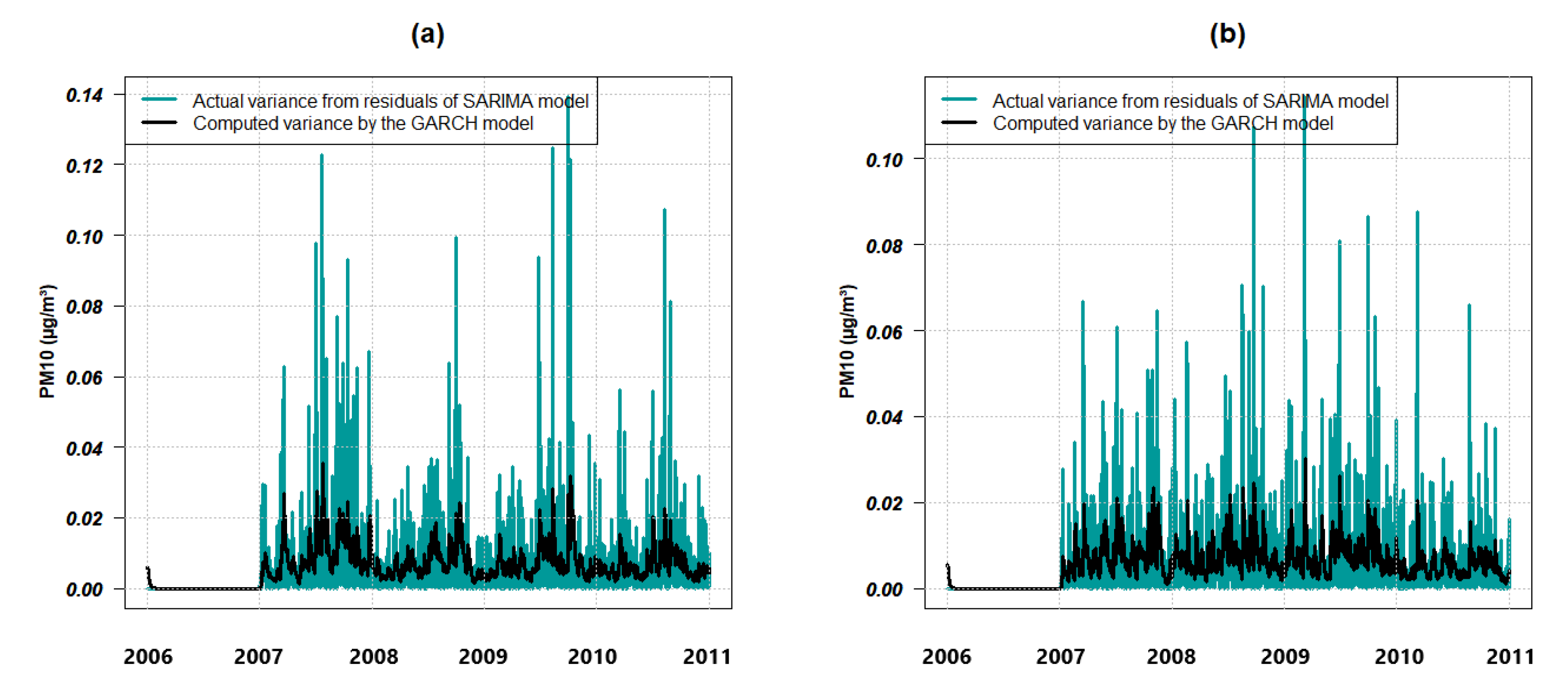
Figure 15 and Figure 16 show the conditional variances estimation of the squared residuals from the $SARIMA$ model and the computed GARCH one. We therefore observed a kind of collinearity between them.

3.7. Forecasting of the PM10 Model

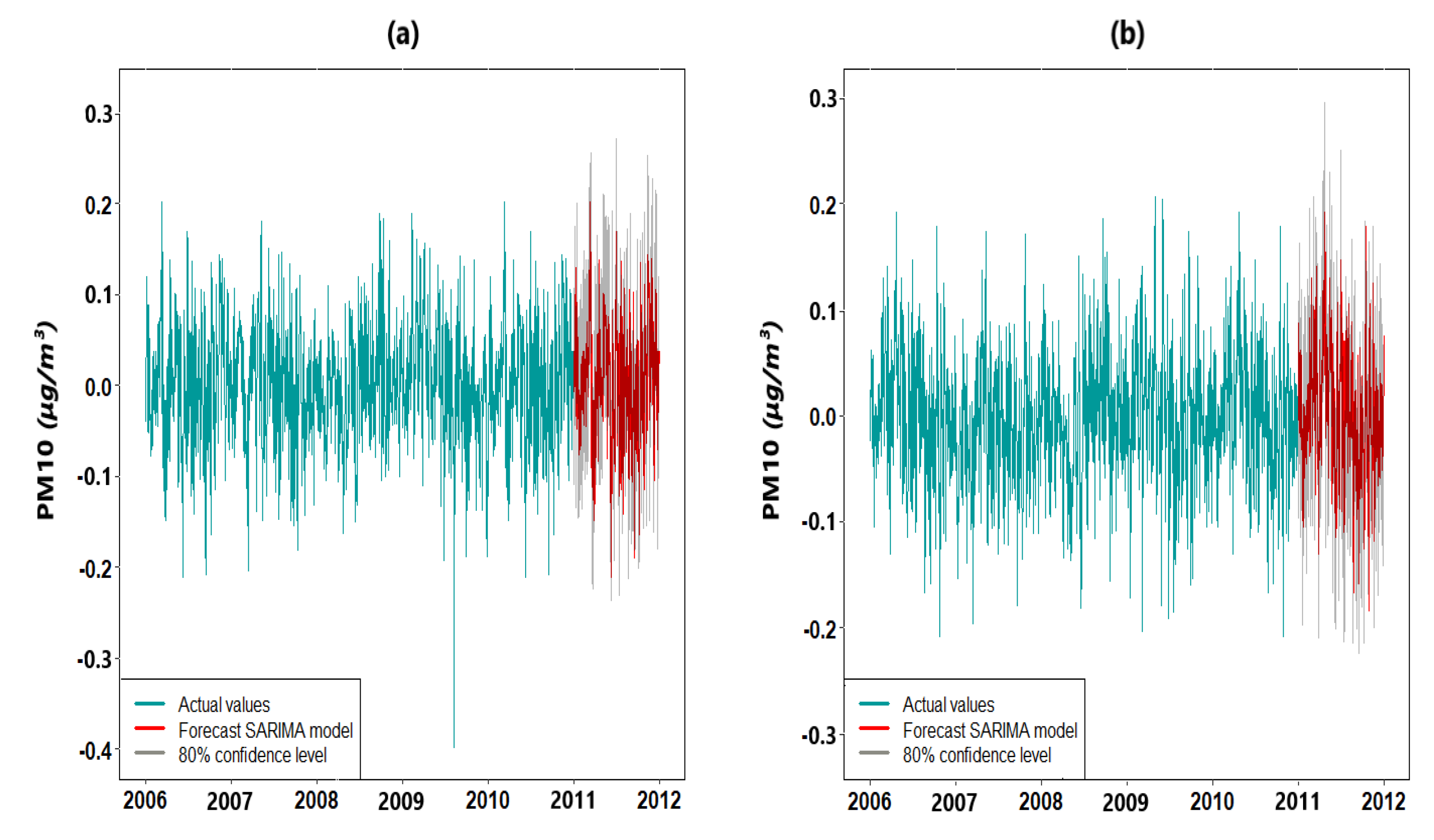
After calibrating the model with five years of data, we perform the forecast in this section. The red curve in Figure 17 illustrates the prediction of the SARIMA model, contained in the 80% confidence interval (light gray). It shows the stochastic nature of PM10 concentration throughout time.

The predicted values from the coupled SARIMA-GARCH model for PM10 on both islands are validated by the forecast error measurements contained in

Table 8. Forecast accuracy of PM10 models in GPE and PR.

	PM10GPE					PM10PR
Models	$\underset{(\mathbf{data}\mathbf{point})}{\mathit{n}}$	$\underset{(\%)}{\mathit{MAPE}}$	MASE	${\mathit{U}}_1$	${\mathit{U}}_2$	$\underset{(\mathbf{data}\mathbf{point})}{\mathit{n}}$	$\underset{(\%)}{\mathit{MAPE}}$	MASE	${\mathit{U}}_1$	${\mathit{U}}_2$
SARIMA	350	$3.743$	$0.025$	$0.083$	$0.167$	350	$2.312$	$0.009$	$0.034$	$0.070$
GARCH	365	$134.238$	$0.775$	$0.556$	$0.882$	365	$141.817$	$0.773$	$0.551$	$0.884$
Coupled SARIMA-GARCH	350	$15.127$	$0.069$	$0.045$	$0.091$	337	$2.396$	$0.008$	$0.034$	$0.069$

. Forecast accuracy indexes as MASE and Theil’s U statistic are overall lower in the coupled SARIMA-GARCH model compared with the other models separately. The MASE index gives more conclusive results than the MAPE. It is due to the fact that these metrics are computed on transformed PM10 data where both negative values and values close to zero are present [58].

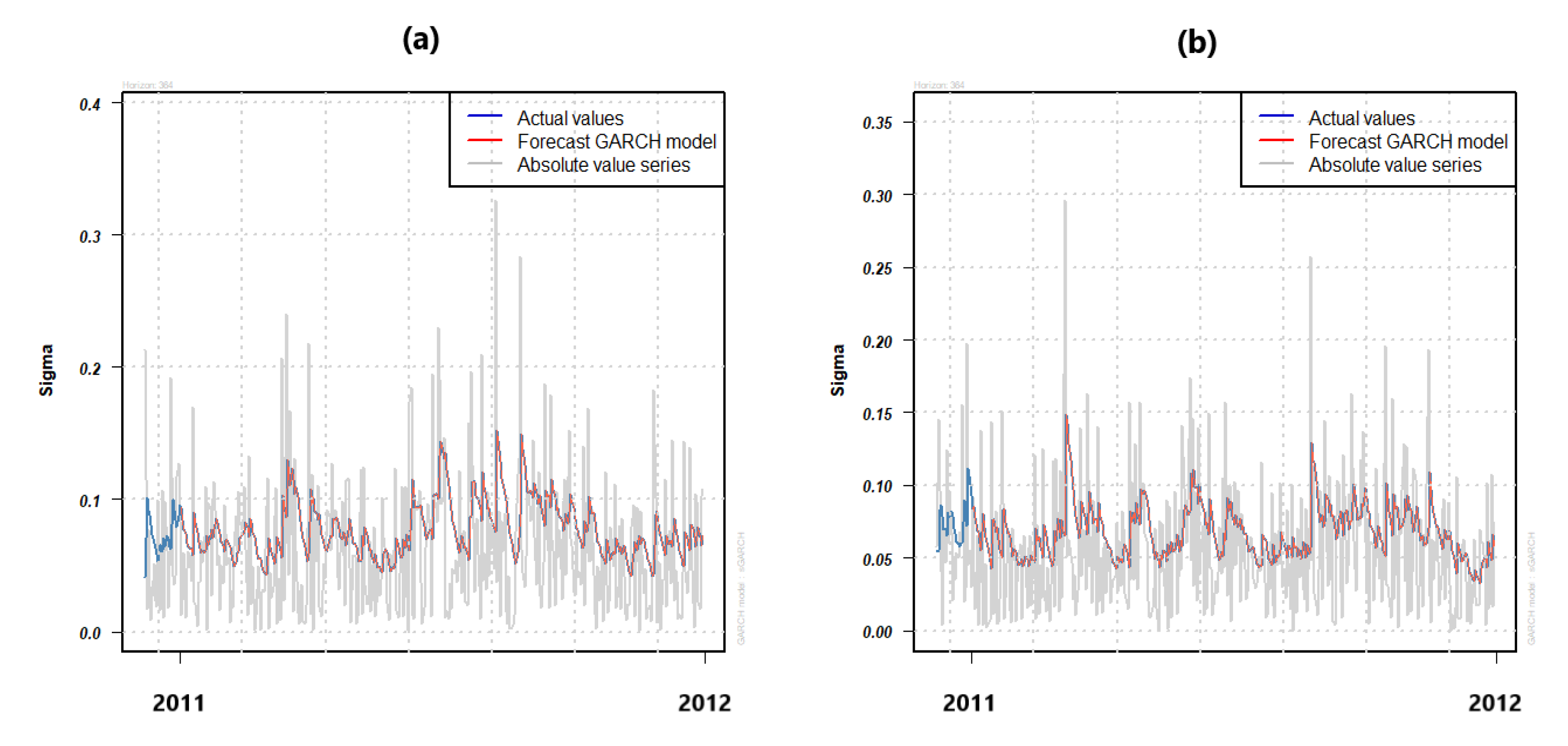
Figure 18 illustrates the GARCH model forecast from standard deviation ${\sigma }_t$. It describes the variability in PM10 365 days after the study period ending in 2010. The concept of the low and high dust seasons is noticeable. We observed a kind of collinearity between the predicted values and those of the residuals from the SARIMA taken in the absolute value.

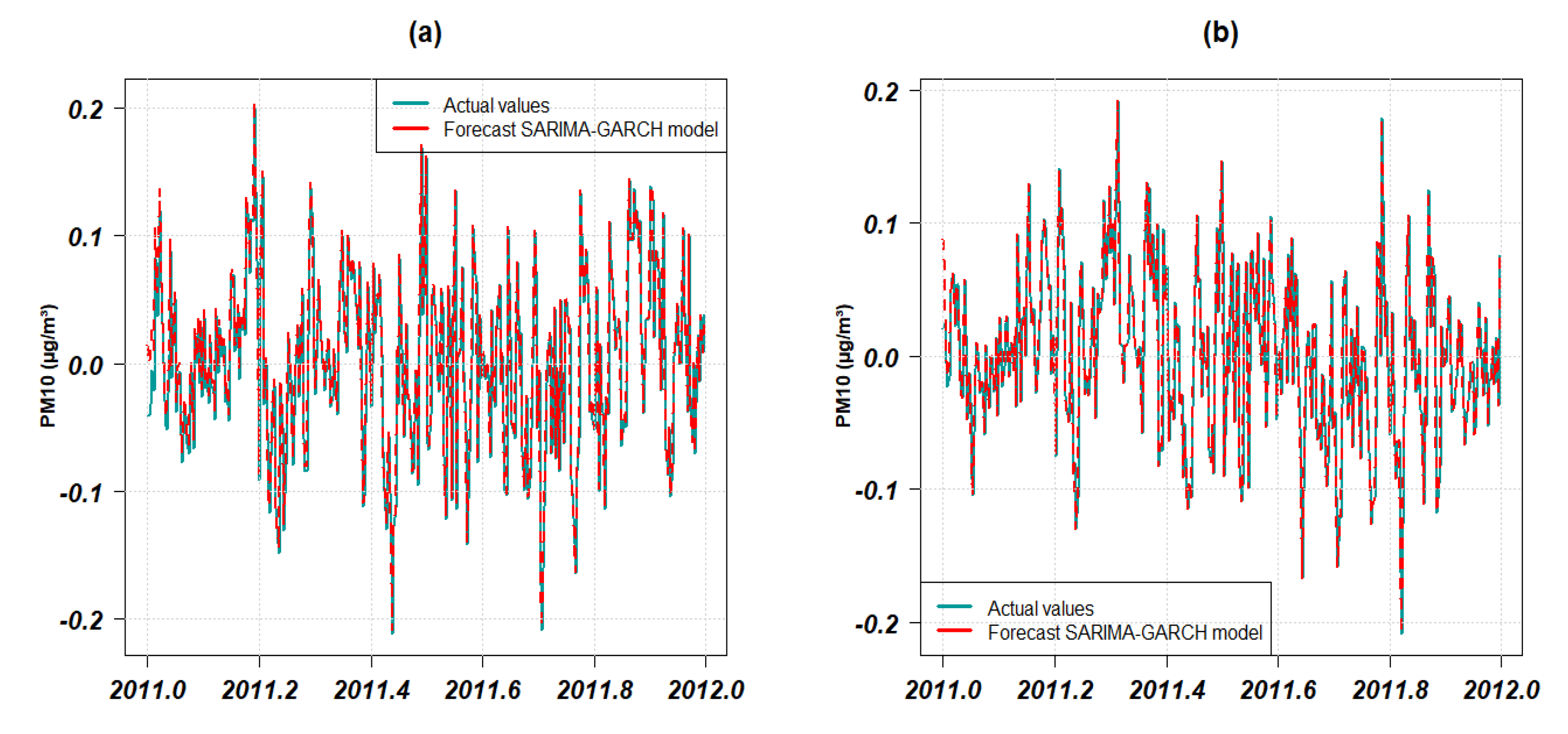
The coupled SARIMA-GARCH model built has an interest compared to the two models applied separately. It concerns the case where the residuals of the SARIMA model have a heteroskedastic behavior. Extreme events related to dust outbreaks or volcanic eruption may explain this behavior. In addition, the values predicted by the coupled SARIMA-GARCH model are obtained by summing the prediction values of both models. All the forecast evaluation indexes in Table 8 confirm that the coupled model is a suitable approach to predict PM10 behavior (see Figure 19 and Figure A4).

4. Conclusions

The goal of this study was to investigate the PM10 behavior in the Caribbean area. To carry out this study, we first replaced the missing data in the time series using the elaborated algorithms, those taking into account the low and high season of the African dust. Thus, the dynamics of the PM10 time series were improved for model building.

Thereafter, the analysis of PM10 stochastic properties was performed using a coupled SARIMA-GARCH model. The SARIMA process allowed us to understand and explain the behavior of the PM10 time series in GPE and PR according to African dust seasonality. The Arch Engle and McLeod–Li tests exhibited the autocorrelations and conditional heteroskedasticity in $SARIMA$ residuals.

The coupled model defined in this study exhibited that PM10 measurements, as well as the residual errors of the SARIMA, reject the normality assumption before and after several transformations. In other words, this model highlights the special features of PM10 concentrations for the Caribbean area. Thus, the SARIMA-GARCH combination is a good tool to forecast PM10 behavior in Caribbean area. The modeling results could be extended to the nearby islands of GPE and PR to better understand the seasonal impact of dust outbreaks on the environment and human health.

In this study, the main difficulty encountered during the modeling process concerns the choice of the model. More precisely, we have had to choose between a hybrid frame and a coupled frame to explain PM10 behavior in GPE and PR. In order to specify the part of the SARIMA and GARCH temporal processes in the hybrid model, a simultaneous estimation of the SARIMA-GARCH parameters is required. To overcome this drawback, the coupled SARIMA-GARCH framework was selected. This latter allowed us to fully model and forecast PM10 fluctuations while independently determining both models’ parameters.

Although our model provides significant results, it is based on an approach with fixed seasonality. It does not take into account long memory processes, those characterized by a decrease in their autocorrelogram following a power function. A future application of this coupled model could be to investigate the impact of mineral dust from African deserts on human health and the environment in Haiti.

References

1. Baughman, R.P.; Culver, D.A.; Judson, M.A. A concise review of pulmonary sarcoidosis. Am. J. Respir. Crit. Care Med. 2011, 183, 573–581. [Google Scholar] [CrossRef] [PubMed] [Green Version]
2. Chen, P.S.; Tsai, F.T.; Lin, C.K.; Yang, C.Y.; Chan, C.C.; Young, C.Y.; Lee, C.H. Ambient influenza and avian influenza virus during dust storm days and background days. Environ. Health Perspect. 2010, 118, 1211–1216. [Google Scholar] [CrossRef] [PubMed] [Green Version]
3. Urrutia-Pereira, M.; Rizzo, L.V.; Staffeld, P.L.; Chong-Neto, H.J.; Viegi, G.; Solé, D. Dust from the Sahara to the American Continent: Health impacts: Dust from Sahara. Allergol. Immunopathol. 2021, 49, 187–194. [Google Scholar] [CrossRef] [PubMed]
4. Matus, K.; Nam, K.M.; Selin, N.E.; Lamsal, L.N.; Reilly, J.M.; Paltsev, S. Health damages from air pollution in China. Glob. Environ. Chang. 2012, 22, 55–66. [Google Scholar] [CrossRef] [Green Version]
5. Manisalidis, I.; Stavropoulou, E.; Stavropoulos, A.; Bezirtzoglou, E. Environmental and health impacts of air pollution: A review. Front. Public Health 2020, 8, 14. [Google Scholar] [CrossRef] [Green Version]
6. Krzyzanowski, M.; Kuna-Dibbert, B.; Schneider, J. Health Effects of Transport-Related Air Pollution; World Health Organization. Regional Office for Europe: Copenhagen, Denmark, 2005; pp. 1–205. [Google Scholar]
7. Choobari, O.A.; Zawar-Reza, P.; Sturman, A. The global distribution of mineral dust and its impacts on the climate system: A review. Atmos. Res. 2014, 138, 152–165. [Google Scholar] [CrossRef]
8. Plocoste, T.; Calif, R. Is there a causal relationship between Particulate Matter (PM10) and air Temperature data? An analysis based on the Liang–Kleeman information transfer theory. Atmos. Pollut. Res. 2021, 12, 101177. [Google Scholar] [CrossRef]
9. Plocoste, T. Multiscale analysis of the dynamic relationship between particulate matter (PM10) and meteorological parameters using CEEMDAN: A focus on “Godzilla” African dust event. Atmos. Pollut. Res. 2022, 13, 101252. [Google Scholar] [CrossRef]
10. Fugiel, A.; Burchart-Korol, D.; Czaplicka-Kolarz, K.; Smoliński, A. Environmental impact and damage categories caused by air pollution emissions from mining and quarrying sectors of European countries. J. Clean. Prod. 2017, 143, 159–168. [Google Scholar] [CrossRef]
11. Sonwani, S.; Maurya, V. Impact of air pollution on the environment and economy. In Air Pollution: Sources, Impacts and Controls, 1st ed.; Chapter: 7; CABI Publisher: Oxford, UK, 2018. [Google Scholar]
12. Gurjar, B.R.; Molina, L.T.; Ojha, C.S.P. Air Pollution: Health and Environmental Impacts; CRC Press: Boca Raton, FL, USA, 2010. [Google Scholar]
13. Bokwa, A. Environmental impacts of long-term air pollution changes in Kraków, Poland. Pol. J. Environ. Stud. 2008, 17, 673–686. [Google Scholar]
14. Ljung, G.M.; Box, G.E. On a measure of lack of fit in time series models. Biometrika 1978, 65, 297–303. [Google Scholar] [CrossRef]
15. Box, G.E.; Jenkins, G.M.; Reinsel, G.C. Time Series Analysis Forecasting and Control; Holden-Day: San Francisco, CA, USA, 1976. [Google Scholar]
16. McLeod, A.I.; Li, W.K. Diagnostic checking ARMA time series models using squared-residual autocorrelations. J. Time Ser. Anal. 1983, 4, 269–273. [Google Scholar] [CrossRef]
17. Jacobson, M.Z. Fundamentals of Atmospheric Modeling; Cambridge University Press: New York, NY, USA, 1999. [Google Scholar]
18. Pesaran, M.H. Time Series and Panel Data Econometrics; Oxford University Press: New York, NY, USA, 2015. [Google Scholar]
19. Brockwell, P.J.; Davis, R.A. Time Series: Theory and Methods; Springer Science & Business Media: New York, NY, USA, 2009. [Google Scholar]
20. Pena, D.; Tiao, G.C.; Tsay, R.S. A Course in Time Series Analysis; John Wiley & Sons: Hoboken, NJ, USA, 2011; Volume 322. [Google Scholar]
21. Paolella, M.S. Linear Models and Time-Series Analysis: Regression, ANOVA, ARMA and GARCH; John Wiley & Sons: Hoboken, NJ, USA, 2018. [Google Scholar]
22. Kumar, K.; Jain, V.K. Autoregressive integrated moving averages (ARIMA) modelling of a traffic noise time series. Appl. Acoust. 1999, 58, 283–294. [Google Scholar] [CrossRef]
23. Zafra, C.; Ángel, Y.; Torres, E. ARIMA analysis of the effect of land surface coverage on PM10 concentrations in a high-altitude megacity. Atmos. Pollut. Res. 2017, 8, 660–668. [Google Scholar] [CrossRef]
24. Cujia, A.; Agudelo-Castañeda, D.; Pacheco-Bustos, C.; Teixeira, E.C. Forecast of PM10 time-series data: A study case in Caribbean cities. Atmos. Pollut. Res. 2019, 10, 2053–2062. [Google Scholar] [CrossRef]
25. Martínez-Acosta, L.; Medrano-Barboza, J.P.; López-Ramos, Á.; Remolina López, J.F.; López-Lambraño, Á.A. SARIMA approach to generating synthetic monthly rainfall in the Sinú river watershed in Colombia. Atmosphere 2020, 11, 602. [Google Scholar] [CrossRef]
26. Reisen, V.A.; Sarnaglia, A.J.Q.; Reis, N.C., Jr.; Lévy-Leduc, C.; Santos, J.M. Modeling and forecasting daily average PM10 concentrations by a seasonal long-memory model with volatility. Environ. Model. Softw. 2014, 51, 286–295. [Google Scholar] [CrossRef]
27. Reisen, V.A.; Zamprogno, B.; Palma, W.; Arteche, J. A semiparametric approach to estimate two seasonal fractional parameters in the SARFIMA model. Math. Comput. Simul. 2014, 98, 1–17. [Google Scholar] [CrossRef]
28. Nieto, P.G.; Lasheras, F.S.; García-Gonzalo, E.; de Cos Juez, F. PM10 concentration forecasting in the metropolitan area of Oviedo (Northern Spain) using models based on SVM, MLP, VARMA and ARIMA: A case study. Sci. Total Environ. 2018, 621, 753–761. [Google Scholar] [CrossRef]
29. Bollerslev, T. Glossary to arch (garch). CREATES Res. Pap. 2008, 49, 1–46. [Google Scholar] [CrossRef] [Green Version]
30. Snezhana Georgieva, G.-I.; Atanas, V.I.; Voynikova, D.S.; Boyadzhiev, D.T. Time series analysis and forecasting for air pollution in small urban area: An SARIMA and factor analysis approach. Stoch. Environ. Res. Risk Assess. 2014, 28, 1045–1060. [Google Scholar]
31. de Paula Pinto, W.; Lima, G.B.; Zanetti, J.B. Análise comparativa de modelos de séries temporais para modelagem e previsão de regimes de vazões médias mensais do Rio Doce, Colatina-Espírito Santo. Ciênc. Nat. 2015, 37, 1–11. [Google Scholar]
32. Gocheva-Ilieva, S.; Ivanov, A.; Iliev, I. Exploring key air pollutants and forecasting particulate matter PM10 by a two-step SARIMA approach. In AIP Conference Proceedings; AIP Publishing LLC: Suzhou China, 2019; Volume 2106, p. 020004. [Google Scholar]
33. Jain, S.; Mandowara, V. Study on particulate matter pollution in jaipur city. Int. J. Appl. Eng. Res. 2019, 14, 637–645. [Google Scholar]
34. Zhang, G.; Lu, H.; Dong, J.; Poslad, S.; Li, R.; Zhang, X.; Rui, X. A framework to predict high-resolution spatiotemporal PM2. 5 distributions using a deep-learning model: A case study of Shijiazhuang, China. Remote Sens. 2020, 12, 2825. [Google Scholar] [CrossRef]
35. Islam, M.; Sharmin, M.; Ahmed, F. Predicting air quality of Dhaka and Sylhet divisions in Bangladesh: A time series modeling approach. Air Qual. Atmos. Health 2020, 13, 607–615. [Google Scholar] [CrossRef]
36. Plocoste, T.; Calif, R.; Jacoby-Koaly, S. Temporal multiscaling characteristics of particulate matter PM10 and ground-level ozone O3 concentrations in Caribbean region. Atmos. Environ. 2017, 169, 22–35. [Google Scholar] [CrossRef]
37. Plocoste, T.; Calif, R.; Euphrasie-Clotilde, L.; Brute, F.N. Investigation of local correlations between particulate matter (PM10) and air temperature in the Caribbean basin using Ensemble Empirical Mode Decomposition. Atmos. Pollut. Res. 2020, 11, 1692–1704. [Google Scholar] [CrossRef]
38. Plocoste, T.; Calif, R.; Euphrasie-Clotilde, L.; Brute, F.N. The statistical behavior of PM10 events over guadeloupean archipelago: Stationarity, modelling and extreme events. Atmos. Res. 2020, 241, 104956. [Google Scholar] [CrossRef]
39. Ma, T.; Antoniou, C.; Toledo, T. Hybrid machine learning algorithm and statistical time series model for network-wide traffic forecast. Transp. Res. Part C Emerg. Technol. 2020, 111, 352–372. [Google Scholar] [CrossRef]
40. Kim, Y.; Son, H.G.; Kim, S. Short term electricity load forecasting for institutional buildings. Energy Rep. 2019, 5, 1270–1280. [Google Scholar] [CrossRef]
41. Liang, Y.H. Forecasting models for Taiwanese tourism demand after allowance for Mainland China tourists visiting Taiwan. Comput. Ind. Eng. 2014, 74, 111–119. [Google Scholar] [CrossRef]
42. Weron, R. Electricity price forecasting: A review of the state-of-the-art with a look into the future. Int. J. Forecast. 2014, 30, 1030–1081. [Google Scholar] [CrossRef] [Green Version]
43. Euphrasie-Clotilde, L.; Plocoste, T.; Feuillard, T.; Velasco-Merino, C.; Mateos, D.; Toledano, C.; Brute, F.N.; Bassette, C.; Gobinddass, M. Assessment of a new detection threshold for PM10 concentrations linked to African dust events in the Caribbean Basin. Atmos. Environ. 2020, 224, 117354. [Google Scholar] [CrossRef]
44. Yeo, I.K.; Johnson, R.A. A new family of power transformations to improve normality or symmetry. Biometrika 2000, 87, 954–959. [Google Scholar] [CrossRef]
45. Osborne, J. Improving your data transformations: Applying the Box-Cox transformation. Pract. Assess. Res. Eval. 2010, 15, 12. [Google Scholar]
46. Bickel, P.J.; Doksum, K.A. An analysis of transformations revisited. J. Am. Stat. Assoc. 1981, 76, 296–311. [Google Scholar] [CrossRef]
47. Kwiatkowski, D.; Phillips, P.C.; Schmidt, P.; Shin, Y. Testing the null hypothesis of stationarity against the alternative of a unit root: How sure are we that economic time series have a unit root? J. Econ. 1992, 54, 159–178. [Google Scholar] [CrossRef]
48. Perron, P. Testing for a unit root in a time series with a changing mean. J. Bus. Econ. Stat. 1990, 8, 153–162. [Google Scholar]
49. Schwert, G.W. Tests for unit roots: A Monte Carlo investigation. J. Bus. Econ. Stat. 2002, 20, 5–17. [Google Scholar] [CrossRef]
50. Bourbonnais, R. Econometrics; Dunod: Paris, France, 2003. [Google Scholar]
51. Shumway, R.H.; Stoffer, D.S. Time Series Analysis and Its Applications; Springer: New York, NY, USA, 2000; Volume 3. [Google Scholar]
52. Box, G.E.; Jenkins, G.M.; Reinsel, G.C.; Ljung, G.M. Time Series Analysis: Forecasting and Control; John Wiley & Sons: Hoboken, NJ, USA, 2015. [Google Scholar]
53. Hyndman, R.J.; Athanasopoulos, G. Forecasting: Principles and Practice; OTexts: Melbourne, Australia, 2018. [Google Scholar]
54. Francq, C.; Zakoian, J.M. GARCH Models: Structure, Statistical Inference and Financial Applications; John Wiley & Sons: Hoboken, NJ, USA, 2019. [Google Scholar]
55. Aragon, Y. Time Series with R; EDP Sciences: Paris, France, 2021. [Google Scholar]
56. Shmueli, G.; Lichtendahl, K.C., Jr. Practical Time Series Forecasting with R: A Hands-On Guide; Axelrod Schnall Publishers: Green Cove Springs, FL, USA, 2016. [Google Scholar]
57. Lewis, C.D. Industrial and Business Forecasting Methods: A Practical Guide to Exponential Smoothing and Curve Fitting; Butterworth-Heinemann: Oxford, UK, 1982. [Google Scholar]
58. Hyndman, R.J.; Koehler, A.B. Another look at measures of forecast accuracy. Int. J. Forecast. 2006, 22, 679–688. [Google Scholar] [CrossRef] [Green Version]
59. Bliemel, F. Theil’s Forecast Accuracy Coefficient: A Clarification; SAGE Publications: Los Angeles, CA, USA, 1973. [Google Scholar]
60. Chatfield, C. Time-Series Forecasting; Chapman and Hall/CRC: Boca Raton, FL, USA, 2000. [Google Scholar]
61. Mahmoud, E.; Pegels, C.C. An approach for selecting times series forecasting models. Int. J. Oper. Prod. Manag. 1990, 10, 50–60. [Google Scholar] [CrossRef]
62. Kim, H.Y. Statistical notes for clinical researchers: Assessing normal distribution (2) using skewness and kurtosis. Restor. Dent. Endod. 2013, 38, 52–54. [Google Scholar] [CrossRef]
63. Maumy-Bertrand, M.; Bertrand, F. Introduction to Statistics with R-Third Ed.: Course, Examples, Exercises and Corrected Problems; Dunod: Paris, France, 2018. [Google Scholar]
64. Euphrasie-Clotilde, L.; Plocoste, T.; Brute, F.N. Particle Size Analysis of African Dust Haze over the Last 20 Years: A Focus on the Extreme Event of June 2020. Atmosphere 2021, 12, 502. [Google Scholar] [CrossRef]
65. Cesars, J.; Nuiro, S.; Vaillant, J. Statistical Inference on a Black-Scholes Model with Jumps. Application in Hydrology. J. Math. Stat. 2019, 15, 196–200. [Google Scholar] [CrossRef]
66. Festy, B. Review of Evidence on Health Aspects of Air Pollution—REVIHAAP Project; Technical Report; WHO Regional Office for Europe: Copenhagen, Denmark, 2013; pp. 2268–3798. [Google Scholar]
67. Plocoste, T.; Calif, R. Spectral Observations of PM10 Fluctuations in the Hilbert Space. In Functional Calculus; IntechOpen: London, UK, 2019; pp. 1–13. [Google Scholar]
68. Plocoste, T.; Pavón-Domínguez, P. Temporal scaling study of particulate matter (PM10) and solar radiation influences on air temperature in the Caribbean basin using a 3D joint multifractal analysis. Atmos. Environ. 2020, 222, 117115. [Google Scholar] [CrossRef]
69. Plocoste, T.; Carmona-Cabezas, R.; Jiménez-Hornero, F.J.; de Ravé, E.G. Background PM10 atmosphere: In the seek of a multifractal characterization using complex networks. J. Aerosol Sci. 2021, 155, 105777. [Google Scholar] [CrossRef]
70. Plocoste, T.; Carmona-Cabezas, R.; Jiménez-Hornero, F.J.; de Ravé, E.G.; Calif, R. Multifractal characterisation of particulate matter (PM10) time series in the Caribbean basin using visibility graphs. Atmos. Pollut. Res. 2021, 12, 100–110. [Google Scholar] [CrossRef]
71. Plocoste, T. Detecting the Causal Nexus between Particulate Matter (PM10) and Rainfall in the Caribbean Area. Atmosphere 2022, 13, 175. [Google Scholar] [CrossRef]
Figure 1. Overview of the Caribbean area with the location of Guadeloupe archipelago (16.25° N, −61.58° E; GPE in orange) and Puerto-Rico (18.23° N, −66.50° E; PR in yellow).
Atmosphere 13 00862 g001
Figure 2. Description of the Seasonal ARIMA model [53].
Atmosphere 13 00862 g002
Figure 3. Boxplot of PM10 data in GPE and PR from 2006 to 2010.
Atmosphere 13 00862 g003
Figure 4. Scatterplot and polynomial regression curve in the relationship where (a) (resp. (b)) PM10PR (resp. PM10GPE) is a function of PM10GPE (resp. PM10PR).
Atmosphere 13 00862 g004
Figure 5. Daily evolution of PM10 concentrations at (a) GPE and (b) PR from 2006 to 2010. The red horizontal dashed line shows the Air Quality Guideline for 24 h mean PM10 concentrations at 50 μ g/m 3 [66]. The black curve represents the smoothed moving average series calculated by taking p = 24 .
Atmosphere 13 00862 g005
Figure 6. Additive decomposition of the PM10 data series at (a) GPE and (b) PR from 2006 to 2010.
Atmosphere 13 00862 g006
Figure 7. Autocorrelation function (ACF) of PM10 data at (a) GPE and (b) PR from 2006 to 2010 before the Box–Cox transformation and the seasonal differentiation. The gray vertical lines of equation v = 365 n , n { 1 , 2 , 3 , 4 , 5 } denote the offsets that are multiples of 365.
Atmosphere 13 00862 g007
Figure 8. Chronogram of PM10 data at (a) GPE and (b) PR from 2006 to 2010 after the Box–Cox transformation and the seasonal differentiation.
Atmosphere 13 00862 g008
Figure 9. Fitting of model computed values and transformed data of PM10 in (a) GPE and (b) PR.
Atmosphere 13 00862 g009
Figure 10. Stationarity of the PM10 SARIMA model at (a) GPE and (b) PR from 2006 to 2010.
Atmosphere 13 00862 g010
Figure 11. Chronogram of PM10 SARIMA model residuals in (a) GPE and (b) PR from 2006 to 2010. Selected red and black portions denote locations with high and low residual error variability, respectively.
Atmosphere 13 00862 g011
Figure 12. Chronogram of squared residuals of the SARIMA model of PM10 in (a) GPE and (b) PR from 2006 to 2010.
Atmosphere 13 00862 g012
Figure 13. McLeod–Li test for PM10 model residual errors in (a) GPE and (b) PR from 2006 to 2010.
Atmosphere 13 00862 g013
Figure 14. Shape for distribution of PM10 model residuals at (a) GPE and (b) PR from 2006 to 2010. The red curve is the residual error density, while the green curve is the normal distribution.
Atmosphere 13 00862 g014
Figure 15. Collinearity between variance of residuals from the SARIMA model and computed variance of the GARCH model in (a) GPE and (b) (PR).
Atmosphere 13 00862 g015
Figure 16. Variance of residuals from the SARIMA model against computed variance by the GARCH model in (a) GPE and (b) PR.
Atmosphere 13 00862 g016
Figure 17. Forecasts of PM10 data series in (a) GPE and (b) PR after the Box–Cox transformation and seasonal differentiation. The light gray band represents the 80% confidence interval. The red curves contained in this region are the forecasts beyond 2010.
Atmosphere 13 00862 g017
Figure 18. 365-day rolling forecast of PM10 variability from the GARCH model in (a) GPE and (b) PR.
Atmosphere 13 00862 g018
Figure 19. Actual (blue curve) and predicted (red curve) values plot using the coupled SARIMA-GARCH model for PM10 data transformed in (a) GPE and (b) PR.
Atmosphere 13 00862 g019