
Particulate Matter and Ammonia Pollution in the Animal Agricultural-Producing Regions of North Carolina: Integrated Ground-Based Measurements and Satellite Analysis


Abstract
:1. Introduction
2. Data and Methodology
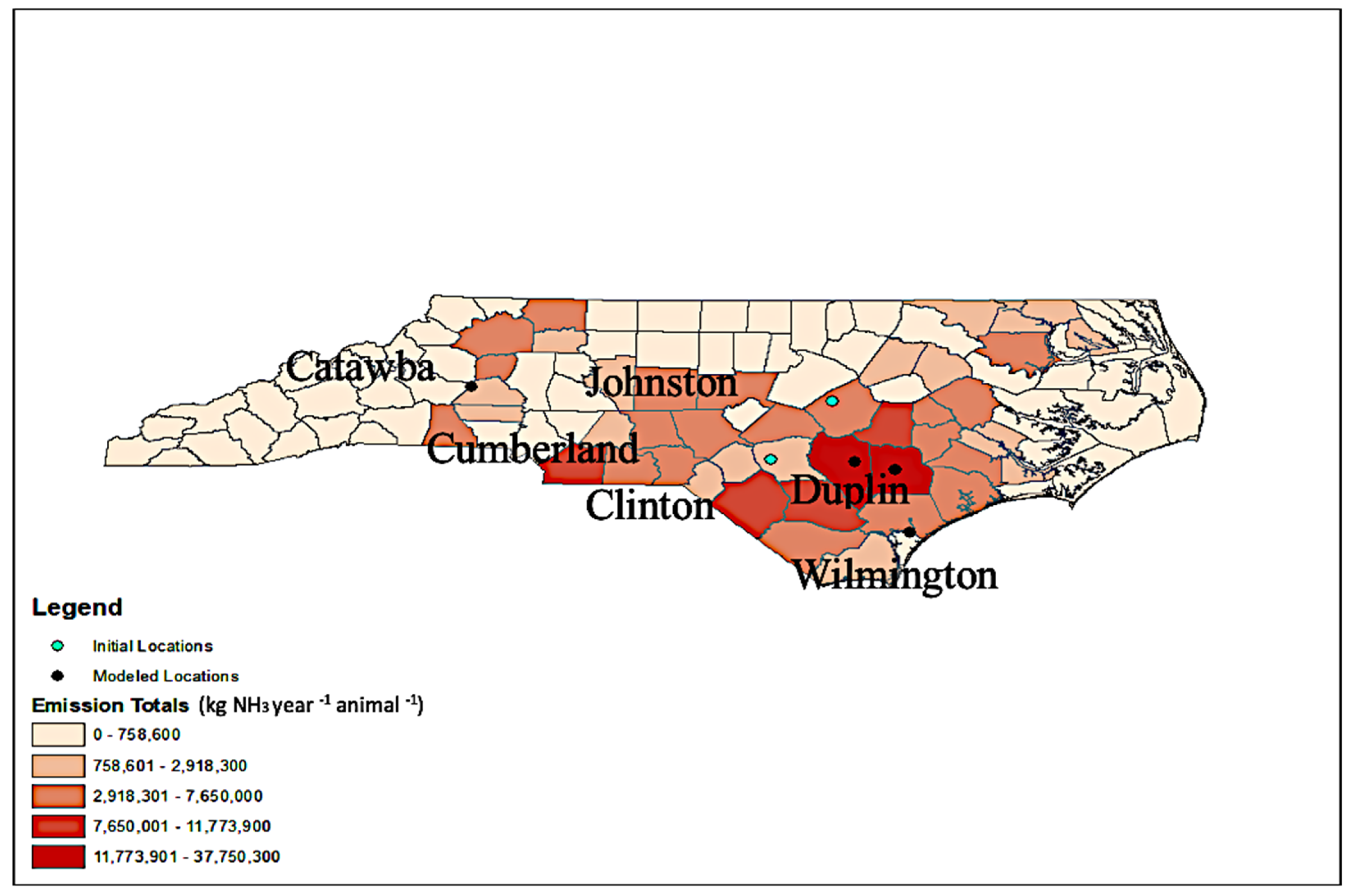
2.1. Location Description
2.2. Satellite-Derived Ammonia Data
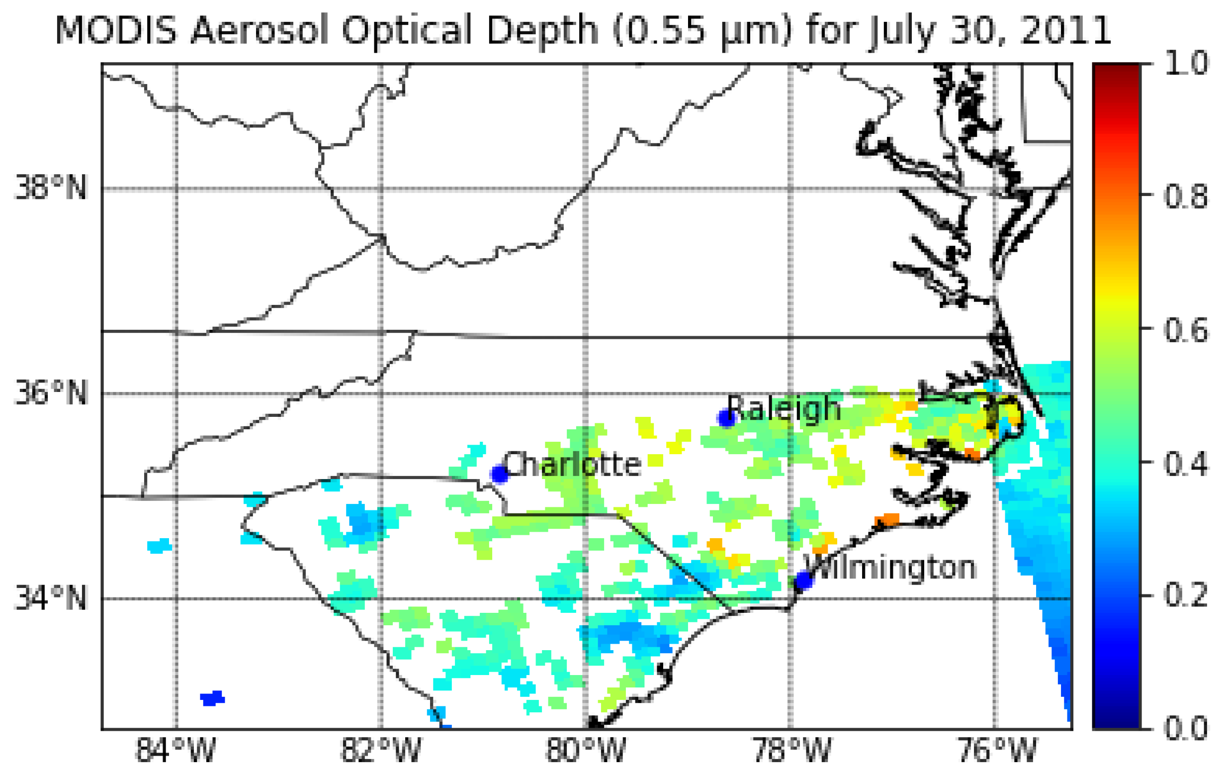
2.3. Satellite-Derived Aerosol Optical Depth
2.4. Ground-Based PM2.5
2.5. Meteorology Data
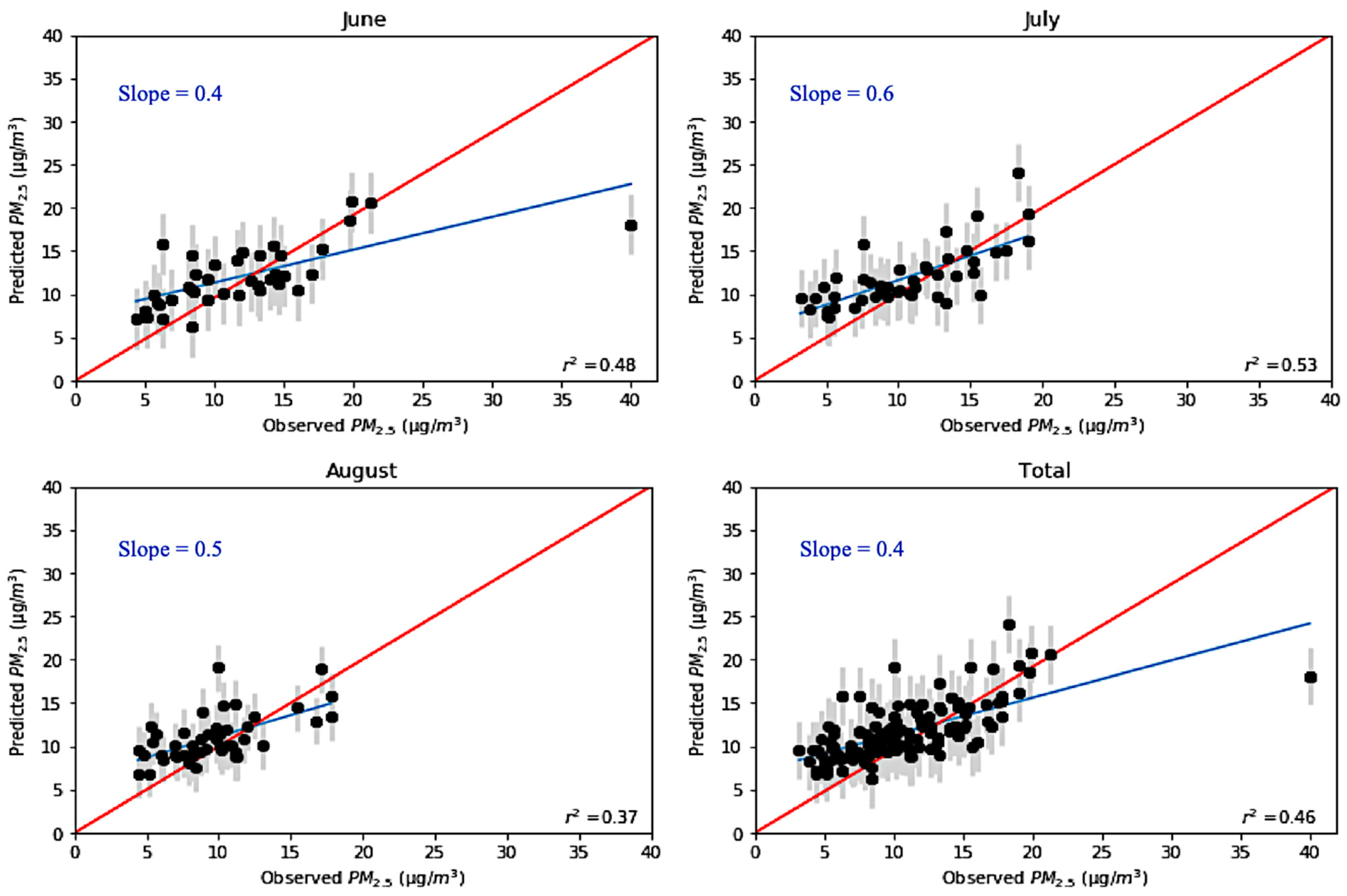
2.6. Methodology
3. Results
4. Conclusions
Author Contributions
Funding
Informed Consent Statement
Acknowledgments
Conflicts of Interest
References
- Aneja, V.P.; Arya, S.P.; Kim, D.S.; Rumsey, I.C.; Arkinson, H.L.; Semunegus, H.; Bajwa, K.S.; Dickey, D.A.; Stefanski, L.A.; Todd, L.; et al. Characterizing ammonia emissions from swine farms in eastern North Carolina: Part 1—Conventional lagoon and spray technology for waste treatment. J. Air Waste Manag. Assoc. 2008, 58, 1130–1144. [Google Scholar] [CrossRef] [PubMed] [Green Version]
- Ross, M. Poultry by the Numbers. Available online: https://sampson.ces.ncsu.edu/2017/11/poultry-by-the-numbers/ (accessed on 7 March 2019).
- United States Department of Agriculture National Agricultural Statistics Service, North Carolina Department of Agriculture and Consumer Science. North Carolina Agricultural Statistics. (Publication No. 218); 2017. Available online: https://www.nass.usda.gov/Statistics_by_State/North_Carolina/Publications/Annual_Statistical_Bulletin/AgStat/NCAgStatBook.pdf (accessed on 30 October 2019).
- Galloway, J.N.; Aber, J.D.; Erisman, J.W.; Seitzinger, S.P.; Howarth, R.W.; Cowling, E.B.; Cosby, B.J. The nitrogen cascade. Bioscience 2003, 53, 341–356. [Google Scholar] [CrossRef]
- Behera, S.N.; Sharma, M.; Aneja, V.P.; Balasubramanian, R. Ammonia in the atmosphere: A review on emission sources, atmospheric chemistry and deposition on terrestrial bodies. Environ. Sci. Pollut. Res. 2013, 20, 8092–8131. [Google Scholar] [CrossRef] [PubMed]
- Faulkner, W.B.; Shaw, B.W. Review of ammonia emission factors for United States animal agriculture. Atmos. Environ. 2008, 42, 6567–6574. [Google Scholar] [CrossRef]
- Aneja, V.P.; Schlesinger, W.H.; Li, Q.; Nahas, A.; Battye, W.H. Characterization of the Global Sources of Atmospheric Ammonia from Agricultural Soils. J. Geophys. Res. Atmos. 2020, 125, e2019JD031684. [Google Scholar] [CrossRef]
- Erisman, J.W.; Bleeker, A.; Galloway, J.; Sutton, M.S. Reduced nitrogen in ecology and the environment. Environ. Pollut. 2007, 150, 140–149. [Google Scholar] [CrossRef] [PubMed] [Green Version]
- Wing, S.; Wolf, S. Intensive livestock operations, health, and quality of life among eastern North Carolina residents. Environ. Health Perspect. 2000, 108, 233–238. [Google Scholar] [CrossRef]
- Aneja, V.P.; Schlesinger, W.H.; Erisman, J.W. Effects of agriculture upon the air quality and climate: Research, policy, and regulations. Environ. Sci. Technol. 2009, 43, 4234–4240. [Google Scholar] [CrossRef] [Green Version]
- Sutton, M.A.; Reis, S.; Riddick, S.N.; Dragosits, U.; Nemitz, E.; Theobald, M.R.; Tang, Y.S.; Braban, C.F.; Vieno, M.; Dore, A.J.; et al. Towards a climate-dependent paradigm of ammonia emission and deposition. Philos. Trans. R. Soc. B Biol. Sci. 2013, 368, 20130166. [Google Scholar] [CrossRef]
- Battye, W.; Aneja, V.P.; Schlesinger, W.H. Is nitrogen the next carbon? Earth’s Future 2017, 5, 894–904. [Google Scholar] [CrossRef] [Green Version]
- Baker, J.; Battye, W.H.; Robarge, W.P.; Arya, S.P.; Aneja, V.P. Characterization and Fate of Ammonia from Poultry Operations: Their Emissions, Transport, and Deposition in the Chesapeake Bay. Sci. Total Environ. 2019, 706, 135290. [Google Scholar] [CrossRef] [PubMed]
- Aneja, V.P.; Arya, S.P.; Rumsey, I.C.; Kim, D.S.; Bajwa, K.S.; Williams, C.M. Characterizing ammonia emissions from swine farms in eastern North Carolina: Reduction of emissions from water-holding structures at two candidate superior technologies for waste treatment. Atmos. Environ. 2008, 42, 3291–3300. [Google Scholar] [CrossRef]
- Aneja, V.P.; Schlesinger, W.H.; Erisman, J.W. Farming pollution. Nat. Geosci. 2008, 1, 409–411. [Google Scholar] [CrossRef]
- Stephen, K.; Aneja, V.P. Trends in agricultural ammonia emissions and ammonium concentrations in precipitation over the Southeast and Midwest United States. Atmos. Environ. 2008, 42, 3238–3252. [Google Scholar] [CrossRef] [Green Version]
- Linker, L.C.; Dennis, R.; Shenk, G.W.; Batiuk, R.A.; Grimm, J.; Wang, P. Computing atmospheric nutrient loads to the Chesapeake Bay watershed and tidal waters. JAWRA J. Am. Water Resour. Assoc. 2013, 49, 1025–1041. [Google Scholar] [CrossRef]
- Schiffman, S.S. Livestock odors: Implications for human health and well-being. J. Anim. Sci. 1998, 76, 1343–1355. [Google Scholar] [CrossRef] [Green Version]
- Wilson, S.M.; Serre, M.L. Examination of atmospheric ammonia levels near hog CAFOs, homes, and schools in Eastern North Carolina. Atmos. Environ. 2007, 41, 4977–4987. [Google Scholar] [CrossRef]
- Bittman, S.; Mikkelsen, R. Ammonia emissions from agricultural operations: Livestock. Better Crops 2009, 93, 28–31. [Google Scholar]
- Aneja, V.P.; Arya, S.P.; Rumsey, I.C.; Kim, D.S.; Arkinson, H.L.; Semunegus, H.; Bajwa, K.S.; Dickey, D.A.; Stefanski, L.A.; Todd, L.; et al. Characterizing Ammonia Emissions from Swine Farms in Eastern North Carolina: Part 2—Potential Environmentally Superior Technologies for Waste Treatment. J. Air Waste Manag. Assoc. 2008, 58, 1145–1157. [Google Scholar] [CrossRef]
- Baker, J.L. Characterization and Fate of Ammonia from Poultry Operations: Their Emissions, Transport, and Deposition in the Chesapeake Bay. Ph.D. Thesis, North Carolina State University, Raleigh, NC, USA, 2020. [Google Scholar]
- Li, H.; Xin, H.; Burns, R.T.; Hoff, S.J.; Harmon, J.D.; Jacobson, L.D.; Noll, S.; Koziel, J.A. Ammonia and PM emissions from a tom turkey barn in Iowa. In 2008 Providence, Rhode Island, June 29–July 2, 2008; American Society of Agricultural and Biological Engineers: Saint Joseph, MI, USA, 2008; p. 1. [Google Scholar]
- Kwok, R.H.F.; Napelenok, S.L.; Baker, K.R. Implementation and evaluation of PM2.5 source contribution analysis in a photochemical model. Atmos. Environ. 2013, 80, 398–407. [Google Scholar] [CrossRef]
- Kampa, M.; Castanas, E. Human health effects of air pollution. Environ. Pollut. 2008, 151, 362–367. [Google Scholar] [CrossRef] [PubMed]
- Pui, D.Y.; Chen, S.C.; Zuo, Z. PM2.5 in China: Measurements, sources, visibility and health effects, and mitigation. Particuology 2014, 13, 1–26. [Google Scholar] [CrossRef]
- Kravchenko, J.; Rhew, S.H.; Akushevich, I.; Agarwal, P.; Lyerly, H.K. Mortality and health outcomes in North Carolina communities located in close proximity to hog concentrated animal feeding operations. N. C. Med. J. 2018, 79, 278–288. [Google Scholar] [CrossRef] [PubMed]
- Holmes, N.S. A review of particle formation events and growth in the atmosphere in the various environments and discussion of mechanistic implications. Atmos. Environ. 2007, 41, 2183–2201. [Google Scholar] [CrossRef] [Green Version]
- Herb, J.; Nadykto, A.B.; Yu, F. Large ternary hydrogen-bonded pre-nucleation clusters in the Earth’s atmosphere. Chem. Phys. Lett. 2011, 518, 7–14. [Google Scholar] [CrossRef]
- Pinder, W.; Davidson, E.A.; Goodale, C.L.; Greaver, T.L.; Herrick, J.D.; Liu, L. Climate change impacts of US reactive nitrogen. Proc. Natl. Acad. Sci. USA 2012, 109, 7671–7675. [Google Scholar] [CrossRef] [Green Version]
- Seinfeld, J.H.; Pandis, S.N. Atmospheric Chemistry and Physics: From Air Pollution to Climate Change; John Wiley & Sons: New York, NY, USA, 2016. [Google Scholar]
- North Carolina Department of Environmental and Natural Resources, North Carolina Utilities Commission. Implementation of the “Clean Smokestacks Act” (Report No. XII). 2014. Available online: https://files.nc.gov/ncdeq/Air%20Quality/news/leg/2014_Clean_Smokestacks_Act_Report.pdf (accessed on 30 October 2019).
- Makar, P.A.; Moran, M.D.; Zheng, Q.; Cousineau, S.; Sassi, M.; Duhamel, A.; Besner, M.; Davignon, D.; Crevier, L.P.; Bouchet, V.S. Modelling the impacts of ammonia emissions reductions on North American air quality. Atmos. Chem. Phys. 2009, 9, 7183–7212. [Google Scholar] [CrossRef] [Green Version]
- Paulot, F.; Jacob, D.J. Hidden Cost of U.S. Agricultural Exports: Particulate Matter from Ammonia Emissions. Environ. Sci. Technol. 2014, 48, 903–908. [Google Scholar] [CrossRef]
- Gong, L.; Lewicki, R.; Griffin, R.J.; Tittel, F.K.; Lonsdale, C.R.; Stevens, R.G.; Pierce, J.R.; Malloy, Q.G.; Travis, S.A.; Bobmanuel, L.M.; et al. Role of atmospheric ammonia in particulate matter formation in Houston during summertime. Atmos. Environ. 2013, 77, 893–900. [Google Scholar] [CrossRef]
- Stokstad, E. Ammonia pollution from farming may exact hefty health costs. Science 2014, 343, 238. [Google Scholar] [CrossRef]
- Wu, Y.; Gu, B.; Erisman, J.W.; Reis, S.; Fang, Y.; Lu, X.; Zhang, X. PM2.5 pollution is substantially affected by ammonia emissions in China. Environ. Pollut. 2016, 218, 86–94. [Google Scholar] [CrossRef] [PubMed] [Green Version]
- Zhao, Z.Q.; Bai, Z.H.; Winiwarter, W.; Kiesewetter, G.; Heyes, C.; Ma, L. Mitigating ammonia emission from agriculture reduces PM2.5 pollution in the Hai River Basin in China. Sci. Total Environ. 2017, 609, 1152–1160. [Google Scholar] [CrossRef] [PubMed]
- Guo, H.; Otjes, R.; Schlag, P.; Kiendler-Scharr, A.; Nenes, A.; Weber, R.J. Effectiveness of ammonia reduction on control of fine particle nitrate. Atmos. Chem. Phys. 2018, 18, 12241–12256. [Google Scholar] [CrossRef] [Green Version]
- Cheng, T.; Chen, H.; Gu, X.; Yu, T.; Guo, J.; Guo, H. The inter-comparison of MODIS, MISR and GOCART aerosol products against AERONET data over China. J. Quant. Spectrosc. Radiat. Transf. 2012, 113, 2135–2145. [Google Scholar] [CrossRef]
- Boylan, J.W.; Russell, A.G. PM and light extinction model performance metrics, goals, and criteria for three-dimensional air quality models. Atmos. Environ. 2006, 40, 4946–4959. [Google Scholar] [CrossRef]
- Mazzeo, A.; Zhong, J.; Hood, C.; Smith, S.; Stocker, J.; Cai, X.; Bloss, W.J. Modelling the impact of national vs. local emission reduction on PM2.5 in the West Midlands, UK using WRF-CMAQ. Atmosphere 2022, 13, 377. [Google Scholar] [CrossRef]
- Kim, E.; Kim, B.U.; Kim, H.C.; Kim, S. Sensitivity of fine particulate matter concentrations in South Korea to regional ammonia emissions in Northeast Asia. Environ. Pollut. 2021, 273, 116428. [Google Scholar] [CrossRef]
- Liu, Z.; Zhou, M.; Chen, Y.; Pan, Y.; Song, T.; Ji, D.; Chen, Q.; Zhang, L. The nonlinear response of fine particulate matter pollution to ammonia emission reductions in North China. Environ. Res. Lett. 2021, 16, 034014. [Google Scholar] [CrossRef]
- Choi, H.; Sunwoo, Y. Environmental Benefits of Ammonia Reduction in an Agriculture-Dominated Area in South Korea. Atmosphere 2022, 13, 384. [Google Scholar] [CrossRef]
- Megaritis, A.; Fountoukis, C.; Charalampidis, P.; Pilinis, C.; Pandis, S. Response of fine particulate matter concentrations to changes of emissions and temperature in Europe. Atmos. Chem. Phys. 2013, 13, 3423–3443. [Google Scholar] [CrossRef] [Green Version]
- Battye, W.H.; Bray, C.D.; Aneja, V.P.; Tong, D.; Lee, P.; Tang, Y. Evaluating ammonia (NH3) predictions in the NOAA National Air Quality Forecast Capability (NAQFC) using in situ aircraft, ground-level, and satellite measurements from the DISCOVER-AQ Colorado campaign. Atmos. Environ. 2016, 140, 342–351. [Google Scholar] [CrossRef]
- Bray, C.D.; Battye, W.; Aneja, V.P.; Tong, D.; Lee, P.; Tang, Y.; Nowak, J.B. Evaluating ammonia (NH3) predictions in the NOAA National Air Quality Forecast Capability (NAQFC) using in-situ aircraft and satellite measurements from the CalNex. Atmos. Environ. 2010, 163, 65–76. [Google Scholar] [CrossRef]
- Aneja, V.P.; Pillai, P.R.; Isherwood, A.; Morgan, P.; Aneja, S.P. Particulate matter pollution in the coal-producing regions of the Appalachian Mountains: Integrated ground-based measurements and satellite analysis. J. Air Waste Manag. Assoc. 2017, 67, 421–430. [Google Scholar] [CrossRef] [PubMed] [Green Version]
- House Bill 515: An Act to Enact the Clean Water Responsibility and Environmentally Sound Policy Act, a Comprehensive and Balanced Program to Protect Water Quality, Public Health, and the Environment (HB 515); 1997 Session; General Assembly of North Carolina: Raleigh, NC, USA, 1997.
- Van Damme, M.; Wichink Kruit, R.J.; Schaap, M.; Clarisse, L.; Clerbaux, C.; Coheur, P.F.; Dammers, E.; Dolman, A.J.; Erisman, J.W. Evaluating 4 years of atmospheric ammonia (NH3) over Europe using IASI satellite observations and LOTOS-EUROS model results. J. Geophys. Res. Atmos. 2014, 119, 9549–9566. [Google Scholar] [CrossRef] [Green Version]
- Levy, R.C.; Remer, L.A.; Kleidman, R.G.; Mattoo, S.; Ichoku, C.; Kahn, R.; Eck, T.F. Global evaluation of the Collection 5 MODIS dark-target aerosol products over land. Atmos. Chem. Phys. 2010, 10, 10399. [Google Scholar] [CrossRef] [Green Version]
- Shimshock, J.P.; De Pena, R.G. Below-cloud scavenging of tropospheric ammonia. Tellus B Chem. Phys. Meteorol. 1989, 41, 296–304. [Google Scholar] [CrossRef]
- Devore, J.L. Probability and Statistics for Engineering and the Sciences; Brooks/Cole: Belmont, CA, USA, 2011. [Google Scholar]
- Teetor, P. R Cookbook: Proven Recipes for Data Analysis, Statistics, and Graphics; O’Reilly Media, Inc.: Newton, MA, USA, 2011. [Google Scholar]


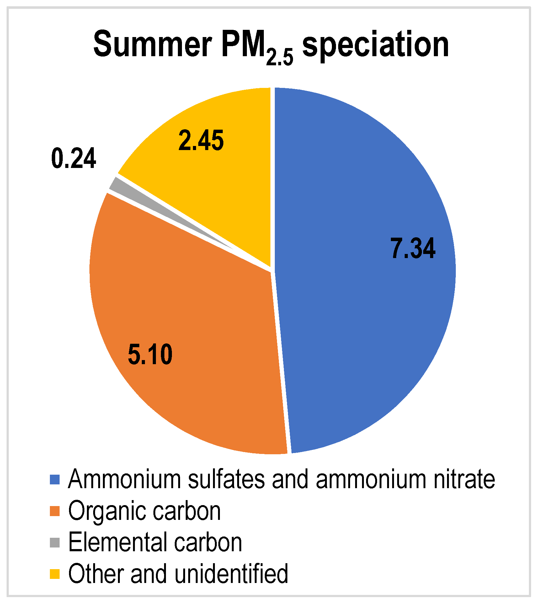
| PM2.5 Composition (µg m−3) | ||
|---|---|---|
| Summer 2006 | Summer 2007 | |
| Ammonium sulfates and ammonium nitrate | 7.08 | 7.34 |
| Organic carbon | 4.44 | 5.10 |
| Elemental carbon | 0.22 | 0.24 |
| Other and unidentified | 2.28 | 2.45 |
| Total | 14.03 | 15.13 |
| Fraction ammonium sulfates and nitrate | 50% | 49% |
| Fraction EC/OC | 33% | 35% |
| Source | DF | Sum of Squares | Mean Square | F Value | Pr > F |
|---|---|---|---|---|---|
| Model | 6 | 18.84 | 3.14027 | 38.99 | <0.0001 |
| Error | 309 | 24.88 | 0.08053 | ||
| Corrected Total | 315 | 43.73 |
| Variable | Parameter Estimate | Standard Error | Type II SS | F Value | Pr > F |
|---|---|---|---|---|---|
| Intercept | 15.14 | 5.07 | 0.72 | 8.92 | 0.0030 |
| Ammonia | 1.05 × 10⁻¹⁷ | 2.99 × 10⁻¹⁸ | 0.98 | 12.21 | 0.0005 |
| AOD | 1.51 | 0.16 | 7.05 | 87.53 | <0.0001 |
| Temp | 0.26 | 0.007 | 1.06 | 13.14 | 0.0003 |
| Pressure | −0.013 | 0.005 | 0.54 | 6.65 | 0.0104 |
| WS | −0.04 | 0.02 | 0.38 | 4.75 | 0.0301 |
| RH | −0.013 | 0.003 | 2.12 | 26.35 | <0.0001 |
| Month | Normalized Mean Bias | Normalized Mean Error |
|---|---|---|
| June | 0.47% | 25.31% |
| July | 13.19% | 24.66% |
| August | 14.59% | 25.23% |
| Month | Normalized Mean Bias | Normalized Mean Error |
|---|---|---|
| June | 17.62% | 28.55% |
| July | 17.70% | 43.61% |
| August | 19.86% | 28.04 |
| Month | Normalized Mean Bias | Normalized Mean Error |
|---|---|---|
| June | −9.68% | 23.92% |
| July | −13.19% | 26.01% |
| August | −14.85% | 27.10% |
Publisher’s Note: MDPI stays neutral with regard to jurisdictional claims in published maps and institutional affiliations. |
© 2022 by the authors. Licensee MDPI, Basel, Switzerland. This article is an open access article distributed under the terms and conditions of the Creative Commons Attribution (CC BY) license (https://creativecommons.org/licenses/by/4.0/).
Share and Cite
Wiegand, R.; Battye, W.H.; Myers, C.B.; Aneja, V.P. Particulate Matter and Ammonia Pollution in the Animal Agricultural-Producing Regions of North Carolina: Integrated Ground-Based Measurements and Satellite Analysis. Atmosphere 2022, 13, 821. https://doi.org/10.3390/atmos13050821
Wiegand R, Battye WH, Myers CB, Aneja VP. Particulate Matter and Ammonia Pollution in the Animal Agricultural-Producing Regions of North Carolina: Integrated Ground-Based Measurements and Satellite Analysis. Atmosphere. 2022; 13(5):821. https://doi.org/10.3390/atmos13050821
Chicago/Turabian StyleWiegand, Rebecca, William H. Battye, Casey Bray Myers, and Viney P. Aneja. 2022. "Particulate Matter and Ammonia Pollution in the Animal Agricultural-Producing Regions of North Carolina: Integrated Ground-Based Measurements and Satellite Analysis" Atmosphere 13, no. 5: 821. https://doi.org/10.3390/atmos13050821
APA StyleWiegand, R., Battye, W. H., Myers, C. B., & Aneja, V. P. (2022). Particulate Matter and Ammonia Pollution in the Animal Agricultural-Producing Regions of North Carolina: Integrated Ground-Based Measurements and Satellite Analysis. Atmosphere, 13(5), 821. https://doi.org/10.3390/atmos13050821