Updated Climatology of Mesospheric Temperature Inversions Detected by Rayleigh Lidar above Observatoire de Haute Provence, France, Using a K-Mean Clustering Technique

Abstract

A climatology of Mesospheric Inversion Layers (MIL) has been created using the Rayleigh lidar located in the south of France at L’Observatoire de Haute Provence (OHP). Using criteria based on lidar measurement uncertainties and climatological mean gravity wave amplitudes, we have selected significant large temperature anomalies that can be associated with MILs. We have tested a novel approach for classifying MILs based on a k-mean clustering technique. We supplied different parameters such as the MIL amplitudes, altitudes, vertical extension, and lapse rate and allowed the computer to classify each individual MIL into one of three clusters or classes. For this first proof of concept study, we selected k = 3 and arrived at three distinct MIL clusters, each of which can be associated with different processes generating MILs in different regimes. All clusters of MIL exhibit a strong seasonal cycle with the largest occurrence in winter. The four decades of measurements do not reveal any long-term changes that can be associated with climate changes and only show an inter-annual variability with a quasi-decadal oscillation.

1. Introduction

The mesosphere, which extends from approximately 50 to 90 km altitude, is a dynamically active layer of the atmosphere which is defined by a negative temperature lapse rate. Due to its high altitude and tenuous nature, the mean thermal state of the air is a complex balance of radiative, dynamical, and some chemical forcing. Above the stratosphere, the constituent gasses of the atmosphere radiate much of the available energy to space. This results in a negative temperature lapse rate with temperatures decreasing with the increasing altitude. Small-scale, fast moving perturbations to the mean radiative mesospheric temperature profile occur commonly as gravity waves (GWs), planetary waves (PWs) and tides displace parcels of air vertically. However, there are also large-scale anomalies lasting several days observed in the mesosphere, which are known as the Mesospheric Inversion Layers (MILs). MILs are large deviations of several tens of Kelvins over several kilometers of altitude, which induce a positive lapse rate of the temperature in the mesosphere.

MILs were first observed by meteorological rockets in the 1970s [1] and were confirmed by other vertical profilers such as Rayleigh lidars [2], sodium temperature lidars [3], falling spheres [4], and satellites [5]. Several mechanisms have been proposed and reviewed [6] for the formation of MILs, but many of the details are still subject to debate.

In a review article, Meriwether and Gardner [6] described two broad classes of MILs.

The first class is the lower MIL, occurring between 65 and 75 km with a summer amplitude of 5 to 10 K and a winter amplitude sometimes exceeding 20 K. It is generally considered that the lower MILs have two formation mechanisms: Firstly, when large, upward-propagating planetary waves reach an altitude where their phase speed matches the speed of the background horizontal wind, the waves break down, dissipate via turbulence, and begin to deposit momentum and energy into the atmosphere. This process acts to slow and potentially reversing the background wind and provide local heating, which reverses the local temperature lapse rate and creates the inversion layer [7]. Secondly, gravity waves can also saturate and interact with the mean horizontal wind in the same fashion as planetary waves. It was further shown by Hauchecorne et al. [2], Le Du, et al. [8] that GWs will preferentially break within a MIL, providing sufficient energy to sustain an inversion with amplitudes up to 40 K. This theory has the added appeal that it can explain seasonal variations in mid-latitude MIL frequencies by relating them directly to their analogues in GW seasonal cycles. Disentangling the relative contributions of PWs and GWs to lower MIL formation is still a relatively open question.

The second class is the upper MIL, occurring in the upper mesosphere with typical amplitudes between 10 and 35 K. This class of MIL is thought to result from non-linear wave breaking and wind–wave interactions [2], as well as from tidal wave breakdown and GW–tidal interactions [9,10]. A third class of MIL was also recently reported by Ramesh et al. [11] in the mesopause region, driven by chemical heating of atomic oxygen. In this paper, we will restrict our analysis to the lower MILs occurring mainly in the lower-middle mesosphere between 60 and 80 km, which are regularly measured by the lidar with high accuracy and precision. Given that what we are presenting is a novel statistical technique for classifying MILs, we will demonstrate our method on the more robust dataset and defer the analysis of upper MILs for a future study.

In general, understanding MIL phenomena and their driving mechanism is important as it can provide insight into the general stability and energy transfer of the middle-atmosphere.

Such a large variability has a large impact on the mean temperature and could probably have a significant impact on decadal trends in the mesosphere. The mesosphere is expected to cool due to the increase in greenhouse gases. In addition, some dynamical feedback is expected as a secondary effect of the climate response due to wave generation and propagation. Cooling is already observed with different sensors [12] and above Observatory of Haute-Provence at mid-latitude [13]. However, multi-decadal, high-resolution datasets of temperature and gravity waves are rare, and MIL occurrence can be a good proxy for assessing long-term gravity wave effects. MILs have a large impact on gravity wave propagation [14], as well as on turbulence [15]) and probably on local wave generation [8]. This huge variability is also a critical issue for atmospheric re-entry either space shuttle, missile, or natural materials such as meteorites [16,17,18,19]. The density vertical profile has a large impact on the trajectory of these objects and also thermal effects, including the potential altitude of the sublimation phase. The phenomenon of meteor ablation from 80 to 110 km allows for the measurement of metal layers by resonance lidars [20] and wind by meteor radars [21].

Addressing the first reason, at the bottom side of the thermal layers (where the temperature profile is increasing in altitude) the positive temperature gradient with increasing altitude signifies an increase in atmospheric stability and reduction in vertical mixing. In contrast, at the top side of the thermal layer, the negative temperature gradient with decreasing altitude implies a reduction in atmospheric stability to the point that the atmosphere may become convectively unstable, thus possibly supporting the development of turbulence [15].

To better understand the cause of MILs, the characteristics of their features need to be better described: altitudes, vertical extension, temperature anomalies, lapse rate, as well as their occurrence frequency. As a tool, we will use the systematic lidar observations performed for more than four decades in the south of France at the Observatory of Haute-Provence [22,23,24] to derive advanced statistical analyses and create an MIL climatology. In this study, we perform a clustering analysis to determined if different types of MILs can be identified by their characteristics. In Section 2, the lidar data and methods are presented. In Section 3, we describe the method used to extract individual MIL characteristics. In Section 4, a climatology of the different MIL parameters is shown. In Section 5, we report the results of a statistical analysis of temperature inversion layers. In Section 6, we describe the results of a new K-mean clustering analysis conducted on ‘MIL families’. In Section 7, we discuss the attributes of these potential MIL families, and finally, in Section 8, we provide some conclusions.

2. Temperature Lidar Observations

Vertical temperature profiles in the middle atmosphere have been obtained with Rayleigh lidar at the Observatory of Haute-Provence (OHP) located in the south of France (44° N, 6° E) within the framework of NDACC network. The Rayleigh lidar temperature datasets were downloaded from the NDACC website (http://www.ndsc.ncep.noaa.gov/). These measurements were set up in the frame of the Network for the Detection of Stratospheric Changes [25] dedicated to stratospheric ozone monitoring.

The dataset consists of a series of nightly temperature profiles from 30 to 80 km starting from 1978 [22]. Routine observations are conducted during clear sky over several hours, mainly at the beginning of the night. The rate of measurements can fluctuate with time; however, due to the quality of the sky transparency and weather, 2–3 measurements per week were obtained. The principle is based on molecular scattering. The method used to retrieve temperature profiles from molecular backscattered signals and the associated errors has been described in detail by Hauchecorne and Chanin [26]. A description of the instrumental error sources and bias has been reported by Keckhut et al. [23]. Temperature uncertainties are negligible in the stratosphere and grow exponentially with decreasing atmospheric density, reaching approximately 5 % near 75 km and 15 % near 90 km. Since 1987, the two existing channels have been mixed together to provide a single signal for the entire height range. This is achieved in comparing both channels in the common altitude range (30–50 km) and in calculating the ratio between both channels and the high-flux nonlinearity of the high-gain channel, considering the low gain channel as a reference. The signal-induced noise (SIN) is considerably reduced using electronic gating, but it can still be identified from the very low mean background noise. It is estimated by fitting with a parabolic function the background signal between 10 km above the top of the temperature profile and 153 km. The residual atmospheric signal at high altitudes is estimated using the MSIS model.

Computation of temperature profiles requires a pressure initialization. Instead of assuming that the pressure at the top of the profile is equal to the value given by the standard atmosphere model, the scale height of the pressure (which is directly related to the temperature) is adjusted in the MSIS model. Part of the actual algorithm can be found in Keckhut et al. [23] and in Singh et al. [27]. Importantly, the accuracy in determining density and temperature is directly related to photon noise and is associated with temporal and vertical resolution. Statistical noise increases with the altitude and becomes suddenly very large as the signal amplitude reaches the noise level. Relative and absolute uncertainties have been identified and quantified using simulated data [28]. Error calculation can be found in Hauchecorne and Chanin [26]. For NDSC purposes, a 2-km vertical resolution constant with altitude is obtained using a Hanning filter. The integration time is about 4 h, depending on weather conditions. The amplitude of the correction of the non-linearities of the counting is determined with an accuracy of 1 K. The error due to the initialization was estimated to be equal to 15% at the initialization level. The calculation of uncertainty shows that this error becomes negligible 15 km below, as opposed to the noise statistic. The sum of these uncertainties is reported in the NDSC archive. The system has undergone successive improvements since its initial construction in 1978 [23]; however, uncertainties remain smaller than ±1 K below 70 km, and potential biases were continuously evaluated with different tools [29], including intercomparisons with a mobile lidar [30].

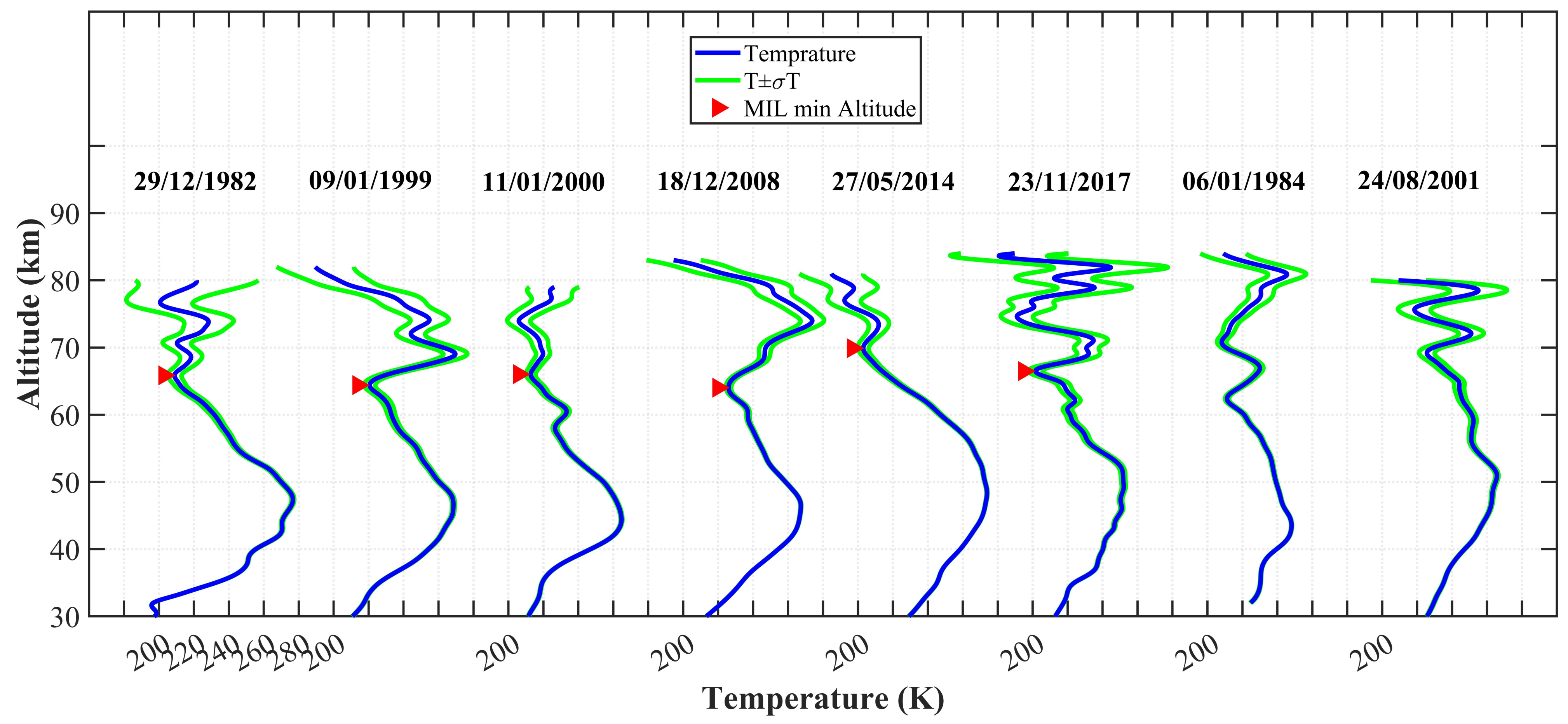
For the present study, the data have been processed using the V6 version of the Temper code developed by LATMOS [31]. The nightly mean profiles from 30 to 90 km have been smoothed over 3 km and interpolated every 1 km are used. The mean thermal profile of the mesosphere is characterized by a regular temperature decrease from the stratopause around 50 km up to the mesopause around 90 km. However, the temperature profiles obtained by Rayleigh lidar in the south of France frequently exhibit near 65 to 70 km a temperature inversion. Examples of nightly mean vertical temperature profiles from the OHP lidar since 1982 have been shown in Figure 1. These temperature profiles indicate temperature inversion layers with different vertical behaviors. The temperature uncertainties have been reduced by vertical and time integration and have been derived with 3 km effective vertical resolution and one sigma error. MILs in the mesosphere, are characterized by a minimum temperature around 60–70 km, with a strong positive gradient above, and a secondary maximum higher up.

3. MILs Detection

Previous studies Hauchecorne et al. [2] already show mesospheric temperature inversions with the OHP lidar and the first statistical characteristics of the mesospheric inversion. In the middle and lower mesosphere, MILs occur at altitudes ranging from 55 to 75 km in winter and 70 to 83 km in summer. Some specific characteristics of MILs such as amplitude and thickness can appear to be similar to other temperature perturbation forcing such as gravity waves or planetary waves. However, MILs tend to persist for several hours to a few days, their vertical extent spans several kilometres, and they can have significantly larger amplitudes compared with gravity waves [32]. However, the exact range of these characteristics is not well-defined. In the examples provided in Figure 1, such a complex issue is obvious. In addition, several MILs can be observed simultaneously. 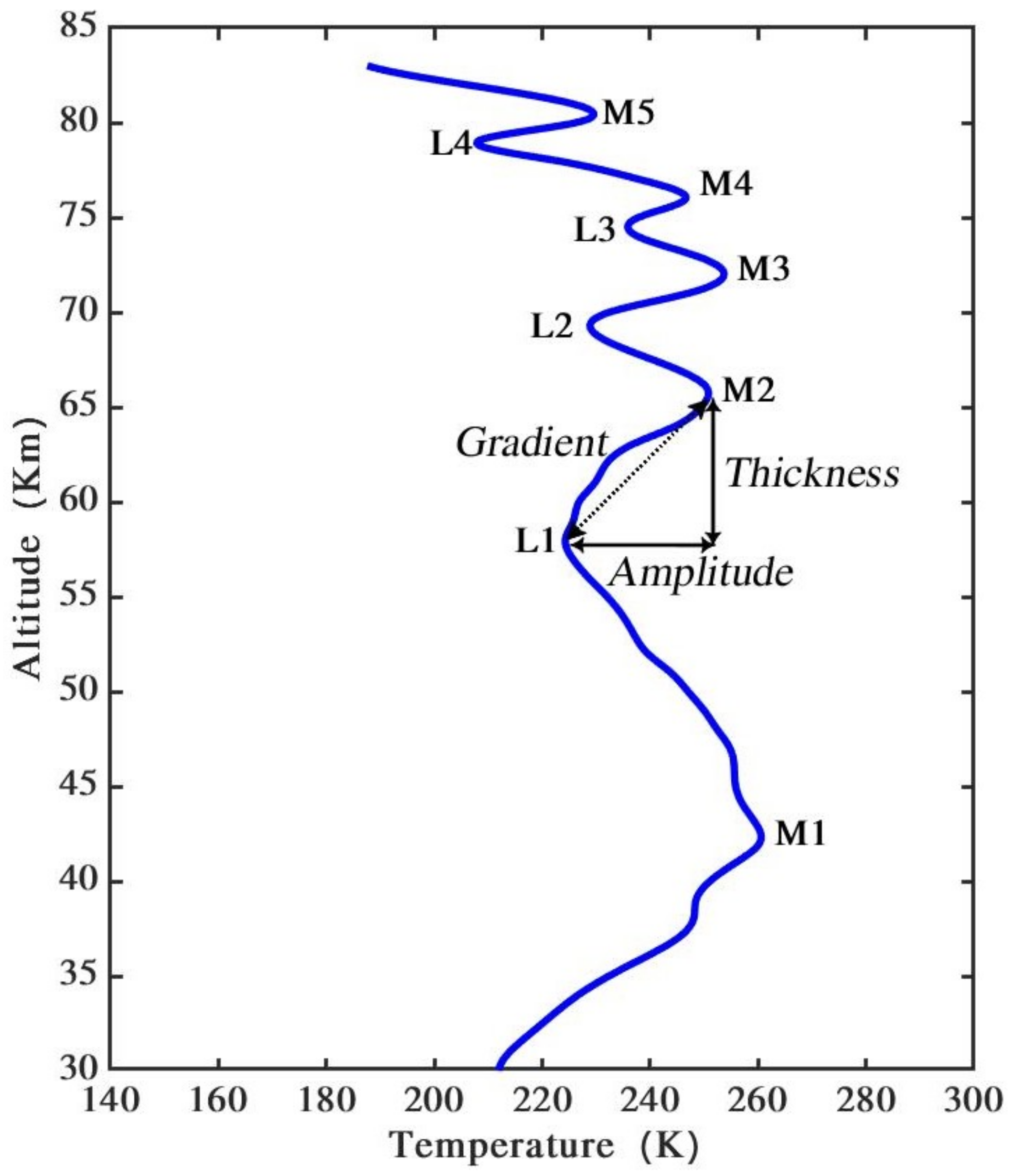The amplitude of an inversions layer was defined by Leblanc and Hauchecorne [5] as the temperature difference between the top and bottom of the inversion layer. The thickness of the inversion layer is the difference between the altitude of the temperature at the top and the altitude of the temperature at the bottom. Therefore, the top and bottom of the inversion layer by the maximum and minimum temperature peaks need to be defined. The bottom part of the MIL is defined as the closest minimum temperature $L_i$ of the ith layer, while the top part is defined by the maximum temperature, $M_i$ as illustrated in Figure 2.

The retrieval of the characteristics of the temperature inversions consists of identifying the minimum and maximum peaks on the temperature graph named as $L_i$ and $M_i$, respectively. To extract the local extremum, a smooth ‘background’ temperature profile is subtracted from the measured temperature profile. The method for estimating temperature extremum is using the derivative of the temperature as a function of altitude, $\overline{T}=\frac{dT}{dz}$ with z considered as the altitude. By horizontal tangent of the temperature graph, the graph of the derivative of the temperature crossing the zero axis $\frac{dT}{dz}=0$.

In the next step, detecting all the maximum and minimum peaks from a temperature profile, the amplitude values, $A_i$, are calculated from the difference between the temperature at the top, $M_i$, and the temperature at the bottom, $L_i$, of the temperature graph:

$$A_i=M_i-L_i$$

(1)

The errors of the maximum temperature and minimum temperature can be used to calculate the amplitude error, $\Delta A$. This estimated error is a quadratic calculation, and accordingly, sigma amplitude is the summation of sigma maximum temperature and sigma minimum temperature. Indeed, the error amplitude, $\Delta A$, is the square root of the sigma amplitudes, and sigma temperatures are the square of Lidar errors, $\Delta Lidar$:

$$\Delta T={(\Delta Lidar)}^2$$

(2)

$${\sigma }_A={\sigma }_{T_{max}}+{\sigma }_{T_{min}}={\sigma }_{M_i}+{\sigma }_{L_i}$$

(3)

$$\Delta A_i=\sqrt{{\sigma }_A}=\sqrt{{\sigma }_{M_i}+{\sigma }_{L_i}}$$

(4)

The thickness values, $H_i$, is the altitude difference between $L_i$ and $M_i$:

$$H_i=Z_{M_i}-Z_{L_i}$$

(5)

For the present study, the nightly mean profiles from 30 to 90 km smoothed over 3 km and interpolated every 1 km are used. Thickness error is the summation of the square root of the squares of maximum altitude and squares of minimum altitude:

$$\Delta H=\sqrt{{\left(Z_{max}\right)}^2+{\left(Z_{min}\right)}^2}$$

(6)

Understanding MIL phenomena is important to the understanding of middle-atmosphere dynamics for two primary reasons: stability and energy transfer. At the bottom side of the thermal layers, where the temperature profile is increasing in altitude, the positive temperature gradient with increasing altitude signifies an increase in atmospheric stability and reduction in vertical mixing. In contrast, at the top side of the thermal layer, the negative temperature gradient with decreasing altitude implies a reduction in atmospheric stability to the point that the atmosphere may become convectively unstable, thus possibly supporting the development of turbulence. Therefore, the temperature gradient $G_i$ with amplitude divided by the thickness was calculated, and the gradient standard error $\Delta G_i/G_i$ is the square root of the squared amplitude error, $\Delta A_i$, divided by amplitude, $A_i$, and squared thickness error $\Delta H_i$ divided by thickness $H_i$:

$$G_i=\frac{A_i}{H_i}$$

(7)

$$\frac{\Delta G_i}{G_i}=\sqrt{{\left(\frac{\mathsf{\Delta }{A}_i}{A_i}\right)}^2+{\left(\frac{\mathsf{\Delta }{H}_i}{H_i}\right)}^2}$$

(8)

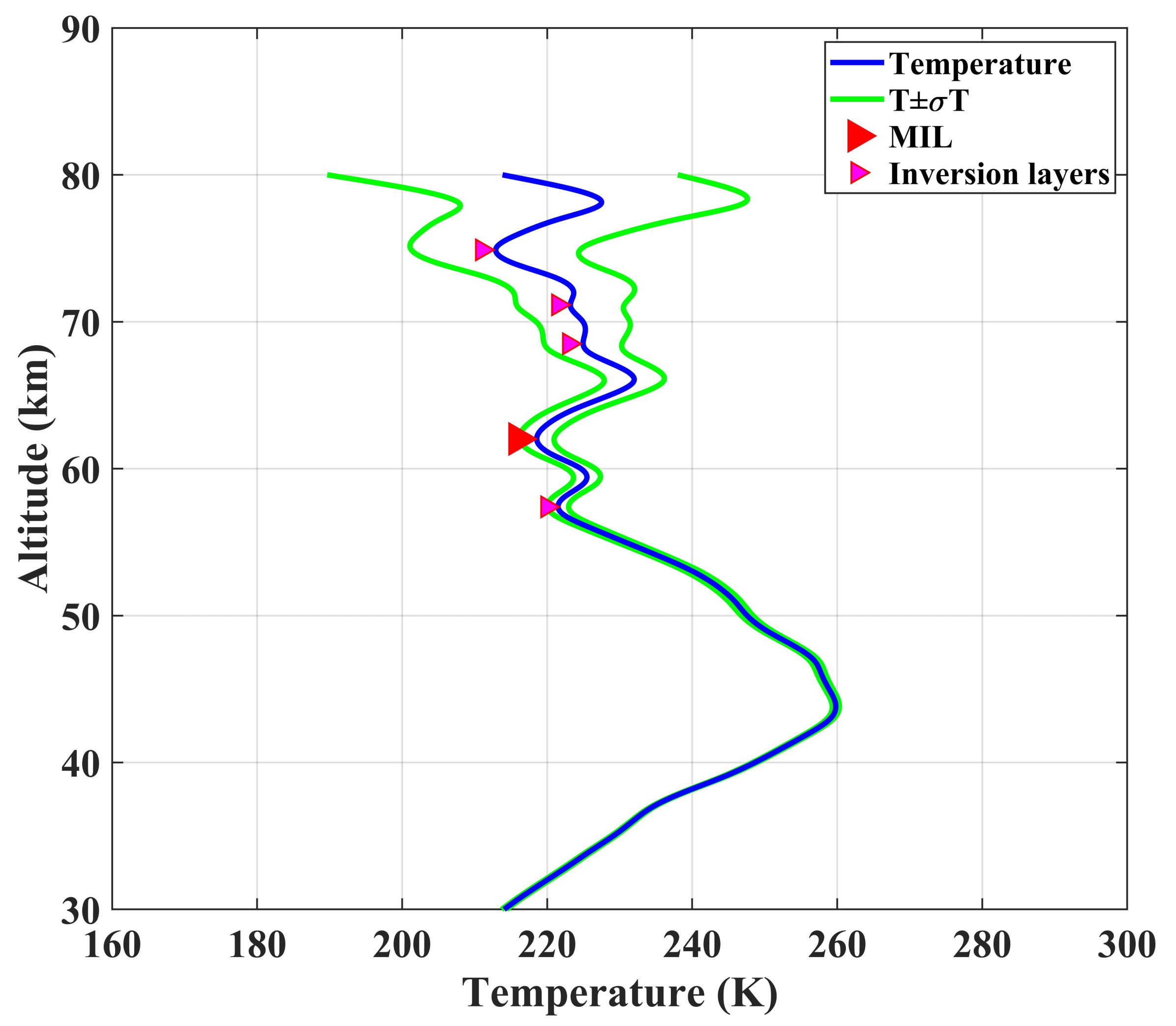
Our primary focus here is detecting the geometric characteristics of individual MILs from the vertical temperature profiles given by lidar observations. An example of determining MIL characteristics from the temperature profile is shown in Figure 3 and

Table 1. Potential MIL anomalies on the vertical temperature profile derived from lidar observation on 4 January 2000.

${\mathit{Z}}_{\mathbf{max}}$ (km)	${\mathit{M}}_{\mathit{i}}\pm \mathbf{\Delta }{\mathit{M}}_{\mathit{i}}$ (K)	${\mathit{Z}}_{\mathbf{min}}$ (km)	${\mathit{L}}_{\mathit{i}}\pm \mathbf{\Delta }{\mathit{L}}_{\mathit{i}}$ (K)	${\mathit{A}}_{\mathit{i}}\pm \mathbf{\Delta }{\mathit{A}}_{\mathit{i}}$(K)	${\mathit{H}}_{\mathit{i}}\pm \mathbf{\Delta }{\mathit{H}}_{\mathit{i}}$(km)	${\mathit{G}}_{\mathit{i}}\pm \mathbf{\Delta }{\mathit{G}}_{\mathit{i}}$ (K/km)
43.85	259.80 ± 0.49	-	-	-	-	-
59.37	225.48 ± 1.84	57.40	221.49 ± 1.45	3.98 ± 2.35	1.96 ± 0.71	2.03 ± 2.80
66.05	232.00 ± 4.13	62.02	218.55 ± 2.39	13.44 ± 4.77	4.02 ± 0.71	3.33 ± 3.42
69.48	225.27 ± 6.06	68.50	224.95 ± 5.36	0.31 ± 8.09	0.98 ± 0.71	0.32 ± 2.34
71.94	223.66 ± 8.25	71.15	223.19 ± 7.44	0.46 ± 11.11	0.78 ± 0.71	0.59 ± 4.17
78.13	227.51 ± 19.81	74.89	212.89 ± 11.63	14.61 ± 22.97	3.24 ± 0.71	4.50 ± 8.50

. This example provides the different characteristics of describing inversions observed on 4 January 2000. Figure 3 shows a clear vertical temperature profile in the 30–90 km altitude range with detected MILs that are marked by red and pink triangles. The amplitude, thickness, and gradient has been calculated according to the mentioned formulas. Based on Table 1, more details of the calculation performed are available. For this case, the maximum value of the amplitude is 14.61 K, and the minimum one is 0.31 K. Importantly, the temperature profiles may be too noisy for considering the detected inversions as significant. In the following sections, the temperature data have been filtered to a vertical resolution of 2 km according to the techniques described in [24]. This has been performed to distinguish between significative MILs and perturbations associated with small-scale GWs and noise. Based on measurement noise, only the inversions from 62 to 66 km are very significative, while the one between 57 and 59 km is just above the threshold given by the noise-estimated level Table 1.

4. MILs’ Climatology

MILs were identified by following the procedure outlined by Leblanc and Hauchecorne [5] and Fechine et al. [33] and is briefly presented here. It is worth noting that this procedure has been applied in many previous studies investigating the phenomenon of mesospheric inversion. A non-exhaustive list of such MIL studies includes: [6,28,34,35,36,37,38]. The identification procedure of Leblanc and Hauchecorne [5] considers the amplitude, thickness, gradient, and altitude of an MIL as the primary characteristics of an inversion layer. The amplitude is defined as the maximum temperature anomaly with respect to a mean ‘unperturbed’ vertical temperature profile. The thickness refers to the vertical extent of the layer spanning the bottomside to topside cold points. The gradient relates how rapidly the temperature of the layer changes over the altitude spanning the MIL. The altitude of the MIL is defined as the altitude of the bottomside cold point below the start of the positive temperature gradient.

In this study, MILs are identified by using the following three criteria:

• The bottom of the inversion is located at least 5 km above the stratopause, and the top is below 90 km;
• The temperature perturbation must be significant within measurement uncertainty;
• The amplitude of the MIL temperature perturbation must be 2$\sigma$ larger than the temperature perturbations expected from gravity waves at the specific altitude

Given that lidars are restricted to zenith viewing, we are unable to see the horizontal extent of the MIL. Likewise, we are restricted to nighttime measurements and are unable to measure a particular MIL continuously over the course of several days. In the context of a lidar measurement, we distinguish between ‘very large gravity waves’ and MILs by utilizing the mean potential energy per unit mass, Equation (9), in order to characterize gravity wave activity, mean temperature deviations can be derived from potential energy following the methods of Wilson et al. [39]:

$$E_p=\frac{1}{2}\frac{g^2}{N^2}{\left(\frac{T^{\prime }}{T}\right)}^2$$

(9)

In the definition of Equation (9), g is the gravitational acceleration, N is the Brunt–Väisälä frequency given in Equation (10), and $(T^{\prime }/T)$ is the atmospheric variance:

$$N^2\left(z\right)=\frac{g\left(z\right)}{T\left(z\right)}\left(\frac{dT}{dz}+\frac{g\left(z\right)}{C_p}\right)$$

(10)

The lidar temperature variance has been computed for each night of our study in the altitude range between 30 km and 85 km. We then calculate a potential energy profile from the mean lidar temperature profile, applying the median and the interquartile range to determine a robust estimator of the $E_p$ variance. We can then compare our nightly average $E_p$ profile to the climatology of potential energy due to the gravity waves observed above the OHP [40]. As a rough estimate for the reader, the climatological $E_p$ at the OHP is around 10 J. kg${}^{-1}$ at 50 km, increasing up to 100 J.kg${}^{-1}$ at 75 km.

In the OHP gravity wave potential energy climatology presented by Mzé et al. [40], the standard temperature deviations at 50 and 75 km are 1.6 and 4 K, respectively. We assume that these fluctuations represent “average gravity wave activity” at OHP. The phenomena we consider to be MILs are much larger in amplitude than even very large gravity waves. We have constructed an altitude dependent cut-off between GWs and MILs based on $2\sigma$. Explicitly, lidar temperature anomalies with amplitudes below 3.2 K at 50 km and 8 K at 75 km are considered as GWs.

As an example of how these selection criteria are applied, Table 1 and Figure 3 shows a list of all parameters determined for the lidar profile from the 4 January 2000. Our algorithm determined five layers in the temperature profile. The first two layers with $z_{m}in$ larger than 57.40 and 62.02 km pass the temperature significance test and have temperature anomalies exceeding the measurement uncertainty. However, the layer at 57.40 km does not exceed our $2\sigma$ potential energy threshold and could be a gravity wave. The second layer at 62.02 km passes both criteria and is labeled as an “MIL” with a large red arrow in Figure 3. The top three layers at $z_{min}$ equal to 68.50, 71.15, and 74.89 all fail the measurement uncertainty criterion.

5. Statistical Analysis of Temperature Inversion Layers

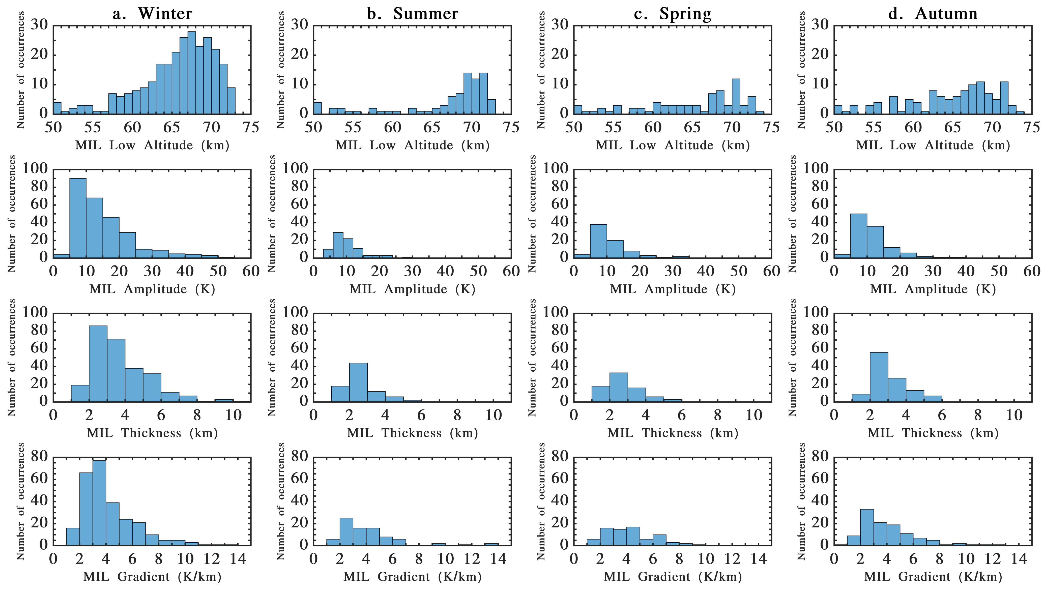
This study has used 4366 OHP nightly Rayleigh lidar observations between 1978 and 2019 to detect MILs. This is a much more robust dataset than has been used in any previous studies of MILs using lidar. Following the MIL detection criteria described in the previous section, 3194 significant inversion layers are detected, and 539 of those layers satisfied the gravity wave $E_p$ criteria in this study. The occurrence distributions of the MIL amplitude, bottomside altitude, layer thickness, and temperature gradient were calculated for each three-month period of summer, winter, spring, and autumn. Figure 4 represents four groups of histograms of the distributions of the MIL’s values to compare seasonal evolutions from 1978 to 2019.

In the first row of Figure 4, we can see that the peak amplitudes of the MILs during winter have a broad, skewed distribution with a maximum near 66 to 70 km. In contrast, the summer maximum is smaller, more narrow, and higher than in the winter, near 69 to 73 km. There does not appear to be a coherent distribution in spring and autumn, giving the reader the visual impression that these periods seem to be transition periods between winter and summer. The absolute number of MIL occurrences measured during the winter months is greater than that measured during the other seasons (see also Figure 5).

In the second row of Figure 4, we can see that the amplitude of the temperature deviation of the MIL also has the largest variability in the winter. Most MILs have amplitudes less than 25 K, but a few can grow as large as 50 K. The spring, summer, and autumn show very similar distributions and are notably different from the winter.

In the third row of Figure 4, we can see that the thickness of the MIL follows the same winter vs. spring–summer–autumn pattern as for the MIL amplitude. Most MILs are thin structures having average vertical extents of 2.5 km; however, some extreme winter layers have a thickness of 8 to 10 km.

In the fourth row of Figure 4, we can see that the gradient of the MIL also follows the same pattern as the previous two MIL variables. If we assume that a typical mesospheric temperature lapse rate might be around 3 K/km, then we can see that summer and spring might have broad normal distributions about the environmental lapse rate. However, it appears that autumn and winter have skewed distributions indicating that complex energy dissipation is happening in these layers.

We can compare our results to a similar study based on 119 nights of Rayleigh lidar observations over an equatorial site from March 1998 to February 2000, Siva Kumar et al. [36]. They showed that the peak occurrence altitudes were between 73 and 79 km (n.b., these authors defined the altitude of the maximum temperature deviation instead of the altitude of the bottomside of the layer, as has been performed in this study). Adjusted for an average MIL thickness of 3–4 km, this result agrees well with our winter results. These authors found the temperature amplitude of the MILs ranged between 12 and 32 K, which again agrees with our winter results.

The inversion frequency is defined as the fraction of the total number of temperature profiles in the month exhibiting one or more inversions. Considering the whole lidar dataset of observations, the frequency of MIL occurrence in winter months (DJF) is much higher than in other seasons.

According to

Table 2. Distribution of MIL measurements by month, 1978–2019.

Month	Season	Number of MILs	Number of Lidar Observation	MIL Detection Ratio (%)	Seasonal MIL Detection Ratio (%)
December		74	388	19.07
January	Winter	122	418	29.18	49.9072
February		73	390	18.71
March		45	405	11.11
April	Spring	14	323	4.33	14.1002
May		17	272	6.25
June		20	326	6.13
July	Summer	32	377	8.48	15.2134
August		30	345	8.69
September		28	391	7.16
October	Autumn	45	353	12.74	20.7792
November		39	378	10.31

, the highest MIL detection ratio is observed during the winter months of December, January, and February (19.07%, 29.18%, and 18.71%, respectively). In contrast, the minimum occurs in the late spring and early summer months of April, May, and June (4.33%, 6.25%, and 6.13%, respectively). March as well as late summer and autumn appear more transitional, having neither maxima nor minima.

This annual wintertime maximum agrees with one of the proposed mechanisms of occurrence of the MILs involving the breaking of gravity waves to sustain the MIL [2]. The lidar and satellite observations reported by Leblanc and Hauchecorne [5] also showed that the frequency of occurrence of MILs follows an annual cycle, with a maximum during the winter months at mid-latitudes and a semi-annual cycle with maxima during the equinoxes at low latitudes. Note that this could also be important earlier in this section, where we compared the distribution of our MIL parameters to those measured by the Gadanki lidar at equatorial latitudes [36].

6. K-Mean Clustering Analyses Applied to MILs

In the previous section, we have seen the broad and sometimes skewed distribution of and seasonal variation in the MIL characteristics. We know from Section 1 that there are several mechanisms proposed for the creation of MILs. Directly linking complex, non-linear, gravity-wave-dissipating phenomena measured by single site Rayleigh lidar systems directly to other quantities such as wave flux is a daunting prospect. Further complications arise, for example, that we do not have simultaneous measurements of the winds and the temperatures and that we cannot work out intrinsic gravity wave parameters or energy dissipation directly.

Given these observational constraints, we wanted to try a different approach and use a clustering technique on this MIL climatology to test the concept of sorting MIL observations into self-similar categories. In this trial study, we will start with a simple K-mean clustering technique, and we will choose k = 3. In the future, we might try a more complex technique with more dynamic variable selection.

Clustering is a descriptive technique [41] when different populations are suspected; therefore, in this study, the k-means clustering method was used for more detailed MIL characteristics analysis to obtain a 3D model of MIL classifications. Cases in the same cluster are similar with respect to the information, cluster analysis was based on variables inducing the dissimilarities. According to the k-means clustering definition, assigning n MIL observations to one of the k clusters is defined by centroids, where k is chosen before the algorithm starts. Then, the point-to-cluster-centroid distances of all observations to each centroid was computed. We should note that to determine distances, the squared Euclidean distance metric has been used. To proceed, an observation was selected uniformly at random from the data set X (main MILs parameters: amplitude, thickness, and minima altitude). The chosen observation is the first centroid and is denoted $c_1$. The next step is computing distances from each observation to $c_1$. The Distance between $c_j$ and the observation m was considering as $d(x_m,c_j)$. The next centroid is selected by $c_2$ at random from X with the probability of P:

$$P=\frac{d^2(x_m,c_1)}{{\sum }_{j=1}^n{d}^2(x_j,c_1)}$$

(11)

To choose center j, at first, the distances from each observation to each centroid are computed, and each observation is assigned to its closest centroid. Thus, for $m=1,\cdots ,n$ and $p=1,\cdots ,j^{-1}$, a centroid j is selected at random from X with probability:

$$P=\frac{d^2(x_m,c_p)}{{\sum }_{h;x_h\in c_p}{d}^2(x_h,c_p)}$$

(12)

where $C_p$ is the set of all observations closest to centroid $C_p$, and $x_m$ belongs to $C_p$. It means each subsequent center is selected with a probability proportional to the distance from itself to the closest center that is already chosen. Therefore, this step is repeated until k centroids are chosen.

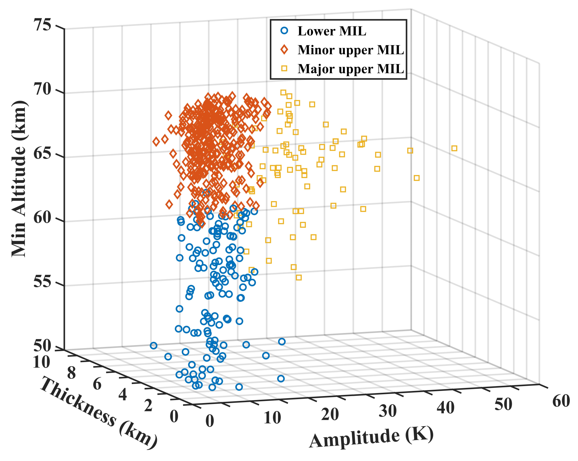
The present study analysis for 42 years of MIL observations, by using the clustering results, tried to classify the characteristics responsible for MIL. In the following, the clustering results reveal three significant MIL groups (Figure 5). The first group with denser data is determined by characteristics such as the minimum height with a maximum peak at 65 km, with a mean amplitude of 9 K, and a thickness between 1 and 6 km with a mean of 3 km (Lower MILs). The second group, minor upper MILs, is located in the middle height range (63–84 km) and has a greater amplitude range in comparison with group 1, from 2 K to 26 K. In addition, the thickness range is larger by 2 to 9 km. Group 3, with more scattered data than the previous two groups, is located in the same altitude range in comparison to group 2, but amplitude is larger than two previous groups (27–60 K) called major upper MILs. The different clusters show significant differences in their amplitude. The first cluster is significantly lower in altitude than the two others. However, similar thicknesses between Groups 2 and 3 are observed, with slightly thicker MILs than group 1. The seasonal behavior of the MIL occurrence shows a full annual cycle for the three categories, with a maximum in winter and a minimum in summer by a factor of 6. Based on the results of each MIL’s group characteristics that are classified in

Table 3. Average values of MIL characteristics separately for each cluster group, 1978–2019.

	MIL Amplitude (K)		MIL min Altitude (km)		MIL Thickness (km)
	Mean	Std	Mean	Std	Mean	Std
Lower MIL	10.9	4.1	57.6	4.1	3.1	1.4
Minor upper MIL	10.3	3.6	68.6	2.5	3.0	1.0
Major upper MIL	27.5	8.1	65.7	3.4	4.5	1.8

, an average of 10.9 K amplitude with 3.1 km thicknesses for Lower MILs calculated in the mean minimum altitude at 57.5 km can be mentioned. However, the mean range values of amplitude for the major upper MIL (27.5 K) are very different from the lower MIL (10.9 K) and the minor upper MILs (10.3 K) values. The overall thickness of major upper MIL and minor upper MIL appears somewhat is evident at first glance that the thickness of major upper MIL (4.5 K) is significantly greater than the other two layers.

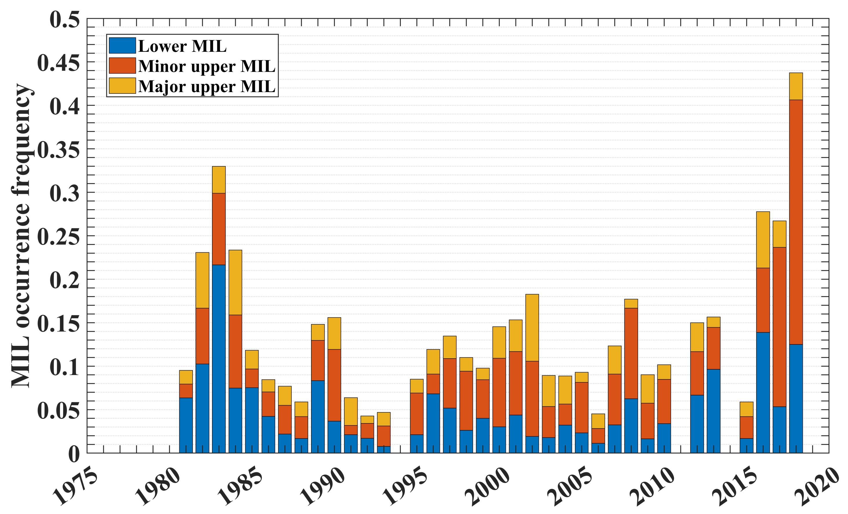
Figure 6 represents the annual evolution of mesospheric inversion layers, showing decadal oscillations. We see local maxima in MIL occurrence in 1981–1983 and 1990–1991 and potentially a minor maxima from 2000–2003 and 2016 to 2019. We speculate that there may be some phase-shifted connection to the solar cycle. The maximum of solar cycle 21 spanned 1976–1979, cycle 22 spanned 1986–1989, cycle 23 spanned 1996-2001, and cycle 24 spanned 2008 to 2014. Previous work [42,43] has well established the connection between mesospheric temperatures and the solar cycle. Going forward, it would be interesting to know the potential role of the solar cycle in the observed fluctuation in MIL.

As an alternative hypothesis, the increase in the number of MIL observations in recent years could be only related to the improved quality of the Rayleigh lidar devices over the years. The variations in the quality of observational sampling of MILs could dominate the time series. Further work is required to investigate this problem.

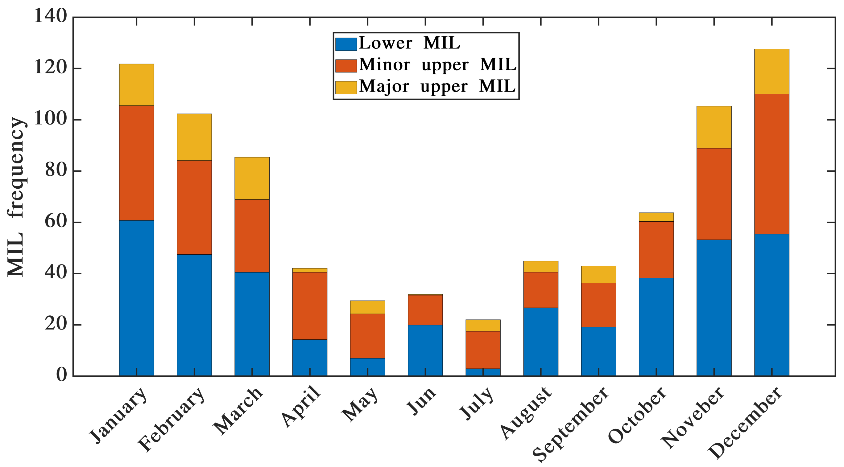
Figure 7 represents the histograms of the MIL frequency (the percentage of times the MILs occurred) for each cluster from 1978 to 2019 by month. Two skewed distributions to the right and left indicate an annual cycle, with most MILs occurring in November, December, January, and February. Note that values greater than 100 account for the detection of multiple MILs during a night, often observed as the ‘double MIL structure’ reported by Meriwether and Gardner [6].

The major upper MILs have a minimum share in monthly distribution, while its maximum is for the lower MIL layer. It is important to mention that the minimum distribution for the lower MIL layer was recorded in July, and no distribution was recorded in June for the significant upper MIL layer. Moreover, the minor upper MIL layer has an almost uniform distribution throughout all months except in June and August. Generally, the distribution of MIL layers has been decreased from April to September. In this work, we have tried a new technique for the classification of MILs. We would like to raise the possibility of using this classification scheme to connect the formation of MILs having different sets of characteristics (i.e., winter, high altitude, thin) to various proposed theoretical mechanisms. In a future work, it would also be interesting to correlate these MIL clusters to other well studied phenomena such as:

• PW breaking, GW breaking and turbulent mixing, and/or GW–tidal interactions that focus GW breaking [7,44,45,46];
• Tropopause and polar-summer mesopause climatological inversions [47,48];
• Reactions to large-amplitude GWs that induce strong wind shears and huge fluctuations in local static stability, as evidenced in stratospheric temperature and wind profiles and MLT [49,50];
• Multiscale dynamics that produce “sheet and layer” structures are easily observable from the surface into the MLT due to wave–wave and wave–mean-flow interactions, instabilities, and turbulence accompanying superposed GWs [51,52,53].

7. Discussion

In this study, we are making a qualitative assessment of mesospheric anomalies that can be associated with mesospheric inversion layer, large anomalies that persist several hours to few days. While three main dynamic phenomena [6] have been proposed to explain these large temperature deviations, there is a question about the attribution of their respective origin. Previous observations suggest that there is a continuum in the altitude of these dynamical anomalies. The statistical analysis of the large anomalies occurring in the mesosphere suggests that these features can be grouped into three classes, yielding multiple regions of strong positive temperature lapse rate on various spatial and temporal scales. The statistical analysis of the large anomalies occurring in the mesosphere above the Observatory of Haute-Provence, as seen by systematic lidar sounding for four decades, suggests that these features can be grouped into three classes. The temperature deviations considered have been separated from smaller anomalies associated either to measurement noise or either to gravity waves. Considering only temperature vertical characteristics, the differentiation between various anomalies with significant positive lapse rates can be found in the altitude of occurrence and their amplitude while the value of the derived temperature positive gradient appears not to be a determinant factor between the different MILs. The seasonal climatology of the MIL occurrence is similar to previous studies and is somehow similar for the different MIL classes. This is not a surprising result, while all the dynamical processes that may be involved in the MIL generation all exhibit a strong seasonal cycle. Whatever the initial cause of MIL generation, either tides, gravity waves, or planetary waves, the dissipation of the gravity waves could maintain a quite stable temperature inversion as the breaking of waves occurs preferably inside and above the inversion layer [2]. Salby et al. [7] seems to indicate that planetary waves could induce MIL. This effect can occur preferably in the lower mesosphere, where the largest anomalies associated with stratospheric warming are observed. These MILs could be associated with the class named Lower MIL. The numerical simulations France et al. [46] have confirmed the role of planetary waves, with, however, a regional response. Tides are the largest in the upper mesosphere. However, Leblanc et al. [54] shows that MILs above California associated with tides occur in the bottom altitude range around 60–65 km but with a very large amplitude. This can be probably associated with the Class 3, named Major upper MILs. Gravity wave breaking occurs above 60 km [40], and then the pure gravity-wave-induced MILs may be associated with the second class called Minor Upper MILs. Thanks to the four decades of measurements above the OHP, the time evolution of the MIL occurrence have been estimated. While all MILs do not reveal any trends that can be associated with any climate change, their evolution has been analyzed according to their classification (Figure 5). A similar behavior can be noted for the lower MIL compare to the global ones. The minor upper MILs reveal a positive trend, while their increase is not significant, as it is mainly observed after 2016. The major upper MILs category shows a nearly constant occurrence, showing that lidar detection is not biased by the detection capability of the lidar that has known some changes since the beginning of the series [23,24].

8. Conclusions

The characteristics of mesospheric inversion layers in the high stratosphere and mesosphere over OHP are the focus of this research. Seasonal trends and variability were studied using the OHP dataset over a lengthy period of time, from 1978 to 2019. In the high stratosphere and lower mesosphere, we confirmed an annual cycle, with a maximum in winter and a minimum in summer. The lidar observations showed night-to-night fluctuations, as well as inter-annual variability in the mesospheric inversion layers. Based on 42 years of Rayleigh lidar data in the middle atmosphere (30–85 km), we also generated mesospheric inversion layer climatology. In addition, the reasons for different classifications of MILs, as well as diverse dynamics that result in the formation of mesosphere inversion layers, were attempted to be clarified (MILs). Finally, we analyzed the seasonal variations in the mesospheric inversion layer activity that observed the dissipation of gravity waves in all seasons. The long-term changes appear to be more difficult to be interpreted either the total MIL occurrence or derived according to the classes, showing at least above OHP that there is no climate evidence associated with MIL occurrence suggesting also no significative climate effect on gravity wave interaction with the mean flow. Attribution of MIL categories to formation processes is not obvious. Analyses with global data with frequent observations will be required using a satellite constellation, for example, [55]. Another alternative is to use much more measured parameters to clarify the processes involved, and the combined analyses of temperature and wind could be also a good indicator of the spatial MIL extensions and then the related processes of either tides, gravity waves, or planetary waves.