Article

An Observing System Simulation Experiment (OSSE) to Study the Impact of Ocean Surface Observation from the Micro Unmanned Robot Observation Network (MURON) on Tropical Cyclone Forecast

1
School of Meteorology, University of Oklahoma, Norman, OK 73072, USA
2
Weathernews Inc., Chiba 261-0023, Japan
*
Authors to whom correspondence should be addressed.
Atmosphere 2022, 13(5), 779; https://doi.org/10.3390/atmos13050779
Submission received: 31 March 2022 / Revised: 29 April 2022 / Accepted: 6 May 2022 / Published: 11 May 2022
(This article belongs to the Special Issue Typhoon/Hurricane Dynamics and Prediction)

Abstract

:
The Micro Unmanned Robot Observation Network (MURON) is a planned in-situ observation network over the surface of West Pacific Ocean, and it is designed to sample high spatial and temporal resolution observations of wind and mass fields over the ocean surface. The impacts of MURON observations for Tropical Cyclone (TC) intensity forecast are investigated using Observation System Simulation Experiments. The regional Ensemble Kalman Filter (EnKF) system of Gridpoint Statistical Interpolation is used with the Advanced Research version of the Weather Research and Forecasting model to conduct OSSEs for typhoon Haiyan (2013) while Haiyan goes through rapid intensification. Assimilating MURON observations improves the TC structure and intensity analysis and forecast. The intensity forecast is improved largely due to the correction of initial vorticity and vertical transport of mass flux. The improvement of intensity forecast is attributed largely to the assimilated MURON wind observations when Haiyan is at the tropical disturbance stage, and then by the MURON mass observations when Haiyan enters the tropical storm stage. In addition, our results show that the quality of moisture analysis is sensitive to the choice of the moisture control variable (CV) in the EnKF system. Using the default pseudo relative humidity (PRH) as the moisture CV degrades the accuracy of the moisture analysis. This is likely due to the neglect of updated temperature field during the nonlinear conversion from the PRH CV to the mixing ratio variable and due to the larger deviation of the PRH from Gaussian distribution. The use of mixing ratio moisture CV mitigates these problems.

1. Introduction

In the past several decades, tropical cyclone (TC) track forecasts have improved dramatically [1,2,3] due to the continuous development of numerical modeling and data assimilation (DA) that improved the representation of the meso- and large-scale environment [4]. While TC track forecasts have improved significantly, TC intensity forecasts have shown less improvement over the same periods [5]. Past studies suggest TC intensity is sensitive to the internal dynamics and moist convection in the TC inner core [6,7,8,9,10]. Due to the chaotic nature of these processes, the errors inherent in the initial conditions can lead to rapid growth of intensity forecast error [11,12,13].
Recent studies have shown that the physical processes in the TC boundary layer play an important role in the development and intensification of a TC. The air–sea exchange of momentum, moisture, and heat flux is an essential source to determine TC intensity [14,15,16]. For example, the surface wind can exchange energy through frictional drag and through the evaporation of ocean water [17,18,19,20], and the surface moisture can modulate formation of a deep convective vortex structure in the boundary layer [20,21].
Therefore, in order to better understand the TC intensification process and improve the TC intensity forecasts, high-resolution surface observations of the wind and the thermodynamic fields within the boundary layer near the TC inner core are required [22]. Conventional observations from buoys are available to measure the surface and near surface conditions within the ocean boundary layer routinely. However, these observations typically have a 500–1000 km spacing, which is spatially too coarse to resolve the inner core structure of a TC. Due to flight range constraints, the use of remote sensing and dropsondes onboard reconnaissance aircraft to sample the near surface ocean conditions are limited to storms near landfall.
Infrared surface sensitive channels from instruments onboard satellites can derive valuable information near the ocean surface. However, due to the difficulty of retrieving information under cloudy or rainy conditions [23,24], deriving surface information beneath widespread clouds and precipitation in TCs remains a challenge. Scatterometers on aircraft or polar orbiting satellites are used to derive the wind speed and direction at the ocean surface, which is helpful in estimating the intensity of a TC in most weather conditions [25,26,27]. However, polar orbiting satellites re-visit the same spot only roughly every 12 h, leading to limited temporal resolution. The Cyclone Global Navigation Satellite System (CYGNSS) mission uses scatterometers onboard eight satellites to observe the ocean surface wind, which provides a wide coverage with a high spatiotemporal resolution when compared to individual scatterometer platforms [28,29]. However, scatterometers like CYGNSS are not able to measure the mass field information such as surface air moisture, temperature, and pressure over the ocean [30].
To provide frequent sampling of dynamic and thermodynamic fields near the ocean surface, the Weather News Incorporation (WNI) is developing the Micro Unmanned Robot Observation Network (MURON) system, which can directly measure the surface wind and thermodynamic variables at high resolution over the open water in the West Pacific Ocean. The instrument is expected to function under strong precipitation, such as that associated with TCs. The data collected may improve the accuracy of TC forecasts over the West Pacific Ocean. This study aims to evaluate the effect of the MURON ocean surface observation on TC intensity forecasts using Observing System Simulation Experiments (OSSEs) before mass production of the MURON network designs.
The paper is organized as follows: Section 2 describes the MURON observation system in detail. In Section 3, we describe the configuration of the nature run, and how the MURON observation is simulated using the nature run. Section 4 provides the experimental design, including the model configuration, the DA method, and the experimental configuration. Section 5 describes the OSSEs results for Typhoon Haiyan in 2013, and Section 6 summarizes the results and discusses future work.

2. The MURON Ocean Surface Observation

WNI’s MURON system is an observation network composed of several thousands of micro robots with meteorological sensors to measure surface wind, air temperature, pressure, and humidity (Figure 1). MURON is expected to be deployed in the broad area from 5~25 N° and 130~160 E° with about 30–50 km horizontal resolution and 60 min temporal resolution. The planed deployment region of MURON was determined from accumulated storm track data from 1945 to 2013 from the Japan Meteorological Agency (JMA). This deployment region coincides with the majority of TC genesis and transits. The propulsion system of each robot has been designed to keep the robot at a stationary location in wind speeds up to 40 m s−1 and tidal current up to 3.08 m s−1. These thresholds correspond to Category 1 TCs on the Saffir–Simpson hurricane wind scale. Ocean waves can cause the robots to vibrate and contaminate wind measurements. MURON has been designed to prevent this by applying orientation sensor data with sub-Hertz sampled wind measurements to determine the direction error and remove it. MURON is designed to operate for about three years using its batteries, which are recharged from a solar panel located on top of the robot. Compared to buoy observations, which are existing meteorological sensors over the ocean surface, the design of MURON is optimized in aerodynamics because the only structures exposed to wind are the sensor mast and radio antenna that are thin. Therefore, MURON is less affected by the wind load friction and has less errors in the sensor than the buoy. On the other hand, due to the sophisticated design and advanced sensors of the MURON instrument, individual MURON is expected to be more expensive to maintain than the buoy.

3. OSSE Framework—Nature Run and Simulated Observations

The objective of an OSSE is to estimate the potential impact of new observation platforms on weather and climate numerical predictions before the observing network is fully deployed [31,32]. A well-designed OSSE includes four critical components: the nature run, which is a numerical simulation that is considered the “true” state of the atmosphere in an OSSE, the simulated observations, the assimilation of the simulated observations, and an assessment of the impact of the synthetic observations by comparing forecasts with and without the assimilation. In this section, our case study of Typhoon Haiyan (2013) is discussed, followed by the description of the first two components of the OSSE. The third and fourth components of the OSSE are described in Section 4 and Section 5, respectively.

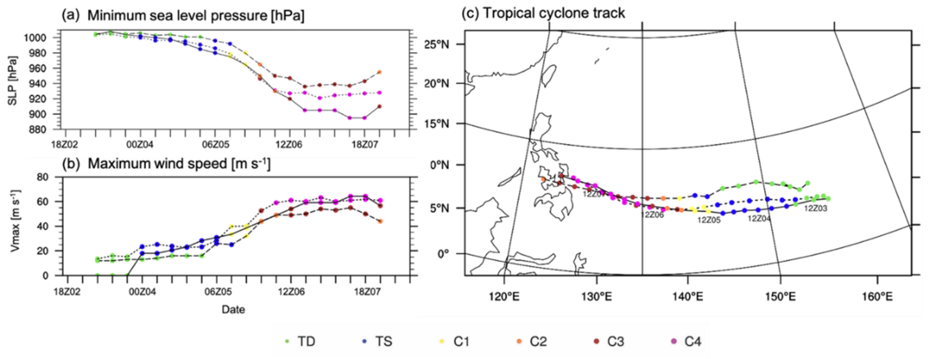
3.1. Case Description: Tropical Cyclone Haiyan (2013)

To evaluate the impacts of the potential new ocean surface observations from MURON on TC intensity forecasts, an OSSE is conducted for Typhoon Haiyan (2013). Haiyan was selected because its rapid intensification (RI) period could be fully sampled by the simulated MURON observations. Typhoon Haiyan (2013) was the most intense TC and the strongest landfalling TC during the 2013 Northwestern Pacific typhoon season. In addition, Haiyan maintained high intensity over an exceptionally long period, which caused serious human and economic devastation in the Philippines. The Joint Typhoon Warning Center (JTWC) first identified it as a tropical disturbance within the monsoon trough at the south of Pohnpei in the Federated States of Micronesia on 2 November 2013. Because of the favorable large-scale environmental conditions with high SST, high moisture content, and weak shear [33], the tropical disturbance further intensified into a low-level cyclonic circulation within 24 h while moving westward. After the system developed into a tropical storm at 0000 UTC on 4 November, it underwent RI. The system obtained typhoon intensity with a surface maximum wind of 36.01 m s−1 at 0000 UTC on 5 November and quickly intensified to 66.88 m s−1 at 0000 UTC on 6 November while tracking westward [34]. The JTWC assessed Haiyan as a Saffir–Simpson category 5 TC on 6 November and reported that the one-minute sustained wind reached 87.45 m s−1 just before Haiyan made landfall in Eastern Samar of the Philippines at 1800 UTC on 7 November. Haiyan maintained category 5 strength during its passing of the Philippines, then weakened slightly on its way across South China Sea as a 61.73 m s−1 cyclone. After the northward deflection, it continued moving inland into southern China where it rapidly dissipated. Recent studies on Haiyan have shown the influence of equatorial wave disturbances on its genesis [33], sensitivity of intensification to the model physical process [35], climatological characteristics [36], contributions of subsurface ocean warming to the RI [37], and the air–sea enthalpy flux conditions contributing to the RI [38].

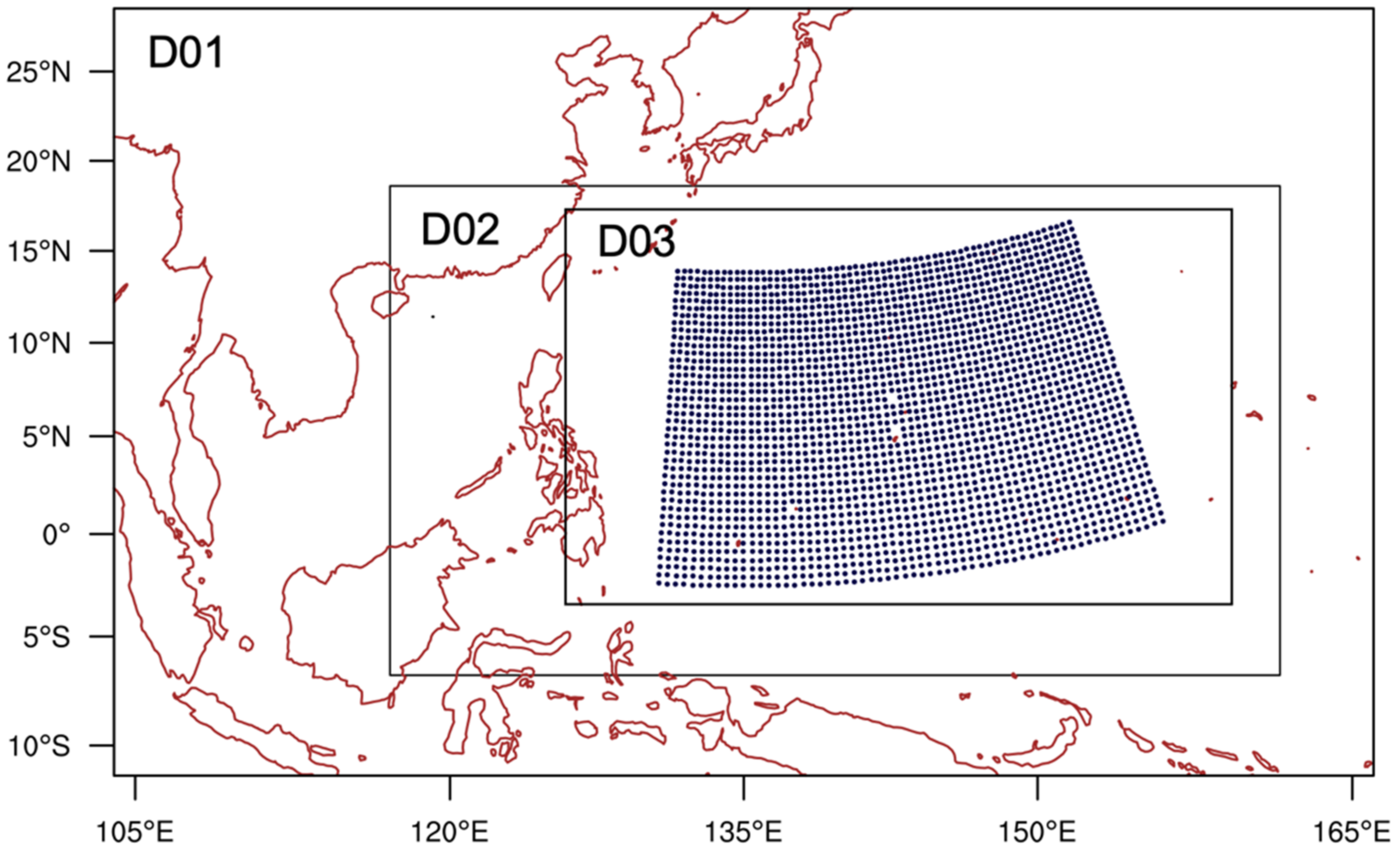
3.2. Configuration of the Nature Run

We ran the Advanced Research version of the Weather Research and Forecasting (ARW-WRF) model version 3.6.1 [39] to simulate TC Haiyan for the OSSE. Three domains of dimensions, 361 × 221 (D1), 763 × 421 (D2), and 1420 × 922 (D3), are used for the simulation with horizontal grid spacings of 27 km, 9 km, and 3 km, respectively (Figure 2). The innermost domain (D3) is set to cover the MURON observation area. Both domains have 40 vertical levels with the model top at 50 hPa. The model was configured with WDM6 microphysics [40], Kain-Fritch cumulus parameterization for D1 and D2 [41,42], Yonsei University (YSU) planetary boundary layer (PBL) scheme [43,44], Noah land surface model [45], Rapid Radiative Transfer Model for Global Climate Models (RRTMG; [46,47]), and longwave and shortwave radiation schemes. It is noted that a convection is explicitly resolved in the innermost domain (D3) without cumulus parameterization. To improve the realism of the nature run, a one-dimensional mixed layer model implemented in WRF was used for the nature run simulation [48,49]. The mixed layer model aims to represent realistic sea surface temperatures by capturing the oceanic upwelling and surface cooling after the passage of TC [49]. The one-dimensional mixed layer model, implemented in WRF3.6.1, treats a grid as a single ocean column [49]. The stratification at the top of the thermocline (Γ) and initial mixed-layer depth (h) should be specified as inputs for this model. We examined the sensitivity of the nature run’s TC intensity to these inputs and set h = 30 m and Γ = 0.1 K m−1, which showed the smallest error in TC intensity simulation. These values are comparable to the previous study [49]. Additionally, to prevent drifting of the simulated nature run track from the analysis, Four-Dimensional Data Assimilation (FDDA) nudging [50], which is implemented in WRF3.6.1, was performed on the outer domain (D1) using the National Centers for Environmental Prediction (NCEP) Global Forecast System (GFS) Final (FNL) analysis (NCEP GFS FNL analysis; http://dss.ucar.edu/datasets/ds083.2, accessed on 30 March 2022) for the first 12-h of the simulation. The FDDA nudging is a gridded analysis nudging that relaxes the nature run fields of horizontal wind, temperature, and humidity to the global GFS FNL analysis during the 12-h nudging period. The purpose of this is to improve the TC initialization by reducing the mismatch between the nature run simulation and the global analysis near the boundaries [49,50]. Previous study found that the FDDA nudging improved the hurricane path simulation especially near the domain boundaries [49]. The nudging time of 12-h was determined to best match TC tracks of the nature run and observations. The NCEP GFS FNL analysis provides initial and boundary conditions for the outer domain (D1), and the model is integrated forward for 144-h starting at 0000 UTC on 2 November 2013 (Figure 3). The nature run is generated by the one-way nested simulation on the 3 km innermost domain (D3).
Because this study focuses mostly on the RI of Haiyan, the nature run was configured for maximizing the accuracy of the onset timing and intensification change during RI. Figure 4 shows the intensity of the nature run and the best-track data from the JMA typhoon center for Haiyan. The nature run catches the onset of the RI process at 0600 UTC 4 November and simulates the intensification of Haiyan measured in terms of the minimum Sea Level Pressure (MSLP) until 0600 UTC 6 November. The nature run simulation shows weaker MSLP than the best track data after 0600 UTC 6 November, likely due to the coarse resolution of the simulation (9 km). Although at a relatively coarse resolution, the nature run shows similar RI timing, intensity change, and storm track to the best track data.

3.3. Simulation of Observation

Simulated MURON ocean surface observations and conventional observations including land surface data, marine surface data, radiosonde data from Global Telecommunication System (GTS), and satellite wind data from National Environmental Satellite data and Information Service (NESDIS) are assimilated in this OSSE. The simulated conventional observations are extracted from the nature run and are interpolated to the corresponding locations and times of the real conventional observations. To obtain simulated MURON observations, the zonal and meridional components of wind, temperature, pressure, and relative humidity of the nature run are interpolated to 2 m above the ocean surface, which is assumed to be the elevation of the MURON sensor in this study. Relative humidity is converted to specific humidity using the temperature and pressure observations following that used in the Gridpoint Statistical Interpolation (GSI) DA system. Hereafter, MURON zonal and meridional wind observations are referred to as “wind” observations, and MURON temperature, pressure, and specific humidity observations are referred to as “mass” observations. Random noise is then added to the interpolated fields. The random noise is drawn from a Gaussian distribution with zero mean and a standard deviation equal to the observational errors. For the conventional observations, we adapt the predefined observation errors used in the operational GSI DA system [51,52]. We estimate the MURON representativeness observation error by inflating the MURON instrument error, similar to [53]. The total MURON observation error is calculated by adding the instrument error and representativeness error. The MURON observational error variance was evaluated in terms of the perspective of the DA experiment in Section 4.4. Table 1 summarizes the observation error variance of MURON (hereafter, MURON_R). Compared to the variance of conventional ocean surface observation used in the GSI system (hereinafter, GSI_R), MURON has larger observation error for pressure, and smaller observation error for temperature, humidity, and wind. The synthetic MURON dataset is encoded into the Global Data Assimilation System (GDAS) prepbufr files for inclusion in the DA cycles.

4. OSSE Framework—Data Assimilation Experiment

4.1. Model Configuration

The same WRF-ARW model and domain configuration as the nature run are used for the DA control runs. To account for the model errors associated with the physical parameterizations, the nature run and the DA run use a different set of physics schemes to the largest extent possible. Previous studies have shown that PBL scheme, microphysics scheme, and cumulus scheme have a significant influence on the simulated TC intensity [54,55,56]. In this study, because the MURON observations measure ocean surface conditions, the DA and control runs are configured with a different PBL scheme than the nature run to accommodate the model errors caused by the lower-tropospheric thermodynamic and kinematic processes. While the nature run used the complex double moment microphysics (WDM6; [40]), the DA and control runs utilized a simple single moment microphysics scheme [37] to represent model errors associated with the formation of clouds and precipitation. The control run and DA runs have the relatively coarse 9 km horizontal resolution and adopt the Kain-Fritsch cumulus scheme [41,42] while the nature run explicitly resolves convection without the cumulus scheme (D3). The control run and DA runs use the Mellor–Yamada–Janjic (MYJ) PBL scheme [57,58,59,60]. The FDDA nudging and the ocean mixed layer configuration are not used by the control and DA runs. The summary of model configurations for the nature run, the control run, and the DA run are presented in Table 2.

4.2. Data Assimilation Method

The GSI Ensemble Kalman Filter (EnKF) system was used for this OSSE study, which uses an ensemble square root filter (EnSRF) algorithm [61]. This algorithm has been used in numerous DA studies for TCs [62,63,64,65,66]. The GSI-based EnKF has been adopted as part of the hybrid EnVar system that is used in the operational GFS model [67,68] and the operational HWRF model [65,66]. The EnSRF algorithm is composed of forecast and analysis steps. During the forecast step, 40 ensemble members are integrated for 6-h to estimate a forecast error covariance that will be used in the analysis step.
At the analysis step, the ensemble mean and ensemble perturbations are updated following Equations (1) and (2) [61], respectively.
x ¯ a = x ¯ b + K y H x ¯ b
x a = x b K ˜ H x b
where the analysis state vector x a and the first-guess (background state) vector x b are composed of the ensemble with a size of K. The ensemble mean of the state vector is denoted by the overbar and the deviation from the mean is denoted by the prime. Here, y denotes the observation, H is the observation operator, and H is the tangent linear of H. K is the Kalman gain defined as K = P b H T H P b H T + R 1 where P b is the background error covariance that is estimated by the background ensemble, and R is the observation error covariance matrix. Here the matrix R is assumed diagonal. K ˜ is the modified Kalman gain defined as K ˜ = α K where α = 1 + R H P b H T + R 1 1 [61].
Sampling error associated with a small ensemble size and a misrepresentation of model error can cause an underestimation of the error variances in the EnKF system, which can result in substantial degradation of the quality of the EnKF analysis and subsequent forecast. To alleviate the problem, covariance localization and inflation techniques are introduced to the GSI EnKF system. The covariance localization technique is applied to the Kalman gain in Equation (1) using the [69] function to remove spurious correlation. The localization technique tapers the analysis increment to zero if the distance between a grid point and an observation is larger than 480 km in the horizontal distance and 1 scale height (i.e., the natural log of the pressure) in the vertical distance for both the outer (D1) and inner domains (D2). The horizontal and vertical cutoff radii of localization are determined to minimize the analysis error averaged over the first 8 cycles for the outer domain (D1). These localization radii are comparable with the previous TC study by [65]. A 3-dimensional multiplicative inflation factor is applied to alleviate the sampling error due to the limited ensemble size. The inflation relaxes the posterior ensemble spread to be 85% of the priori ensemble spread [70,71].

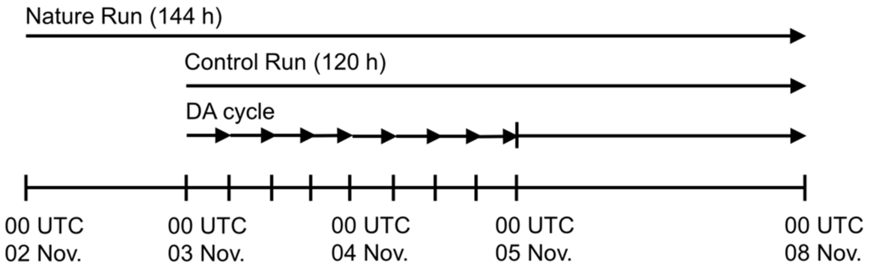
4.3. Data Assimilation Experimental Design

For the control and DA runs, initial conditions (ICs) and lateral boundary conditions (LBCs) for ensemble forecast are generated by adding 40 initial ensemble perturbations to the NCEP GFS FNL analysis at the very beginning of the DA cycles valid at 1800 UTC 2 November 2013. The initial and lateral boundary ensemble perturbations for the outer domain (D1) are sampled from a multivariate normal distribution whose covariance is the pre-generated static forecast error covariance of the WRF 3-dimensional variational DA system (3DVar) [72,73]. They were interpolated to the inner domain (D2) to create ensemble perturbations of ICs for the inner domain (D2). The ensemble of LBCs for the later DA cycles is generated in the same manner. The initial ensemble conditions are integrated for 6 h, and the ensemble mean of the 6-h ensemble forecast is used as the initial condition of the control run valid at 0000 UTC 3 November (Figure 3). The DA run assimilates the simulated conventional observations and MURON observations, while the control run does not. Four sets of DA experiments are conducted to evaluate the effect of different combinations of MURON observed variables on the TC intensity forecasts. The DA_CONV experiment assimilates the simulated conventional observations. The DA_CONV_MURON experiment assimilates both the conventional observations and all observing MURON variables, including surface wind, temperature, specific humidity, and surface pressure. The conventional observations and MURON mass variables, such as surface pressure, temperature, and specific humidity, are assimilated in the DA_CONV_MURON_MASS experiment, and only the MURON horizontal wind components, together with the conventional observations, are assimilated in the DA_CONV_MURON_WIND experiment.

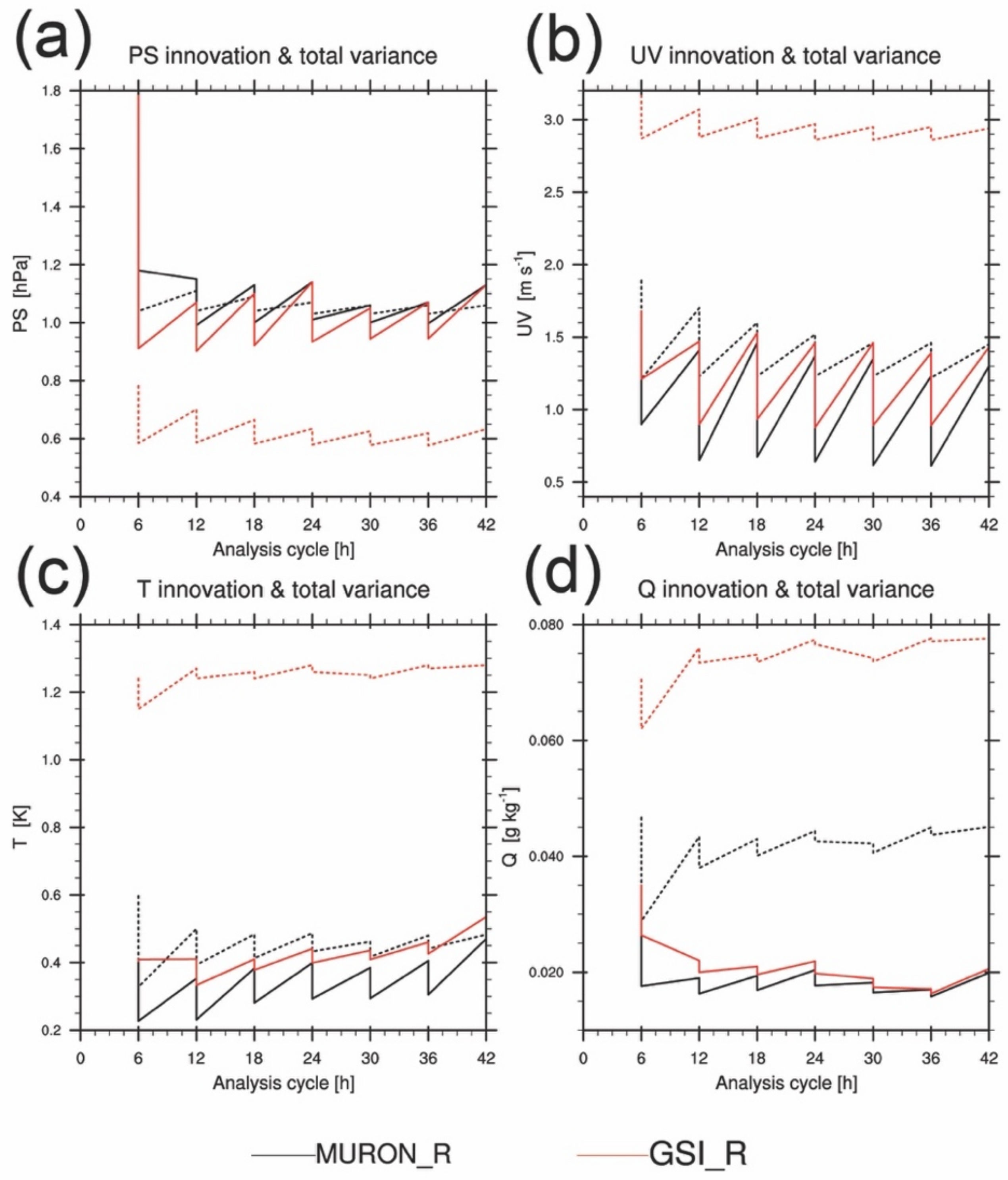
4.4. Choice of Observation Error (GSI_R, MURON_R)

Because proper observation error variance is one of the most important factors for successful assimilation of the new observation, the determination of the MURON observation error variance is based on two diagnostics in observation space. One approach is the Desrozier’s method [74],
E d a o d b o T   = R D ,  
where d a o = y H x ¯ a and d b o = y H x ¯ b are the observation-minus-analysis residual vector and the observation-minus-background (innovation) residual vector, respectively. E is the statistical expectation operator, and R D is the diagnosed observation error variance matrix from Desrozier’s method. Table 1 shows MURON_R, GSI_R, and R D . Compared to R D , both MURON_R and GSI_R overestimate the observation errors, except for the pressure observations. However, MURON_R is more consistent with the diagnosed R D for almost all variables, except for the wind observations compared to GSI_R.
The other approach is based on the following innovation statistics [75].
t r E d b o d b o T   t r H P b H T + t r R ,  
which is commonly used to verify the estimation of error variances from an ensemble. The right side can be defined as the total variance and the left side is as the innovation variance. Different observation error variance estimations are evaluated by examining the degree of agreement between the right and left sides of Equation (4). Figure 5 shows the sawtooth plot using the analysis and 6-h forecast at each cycle. MURON_R results in smaller root-mean-square (RMS) of innovations and a more consistent relationship between the RMS of innovations and the total variance than GSI_R for all variables. Based on these two diagnostics, we have configured all DA experiments to use MURON_R as the observation error covariance R in Equations (1) and (2).

5. Results

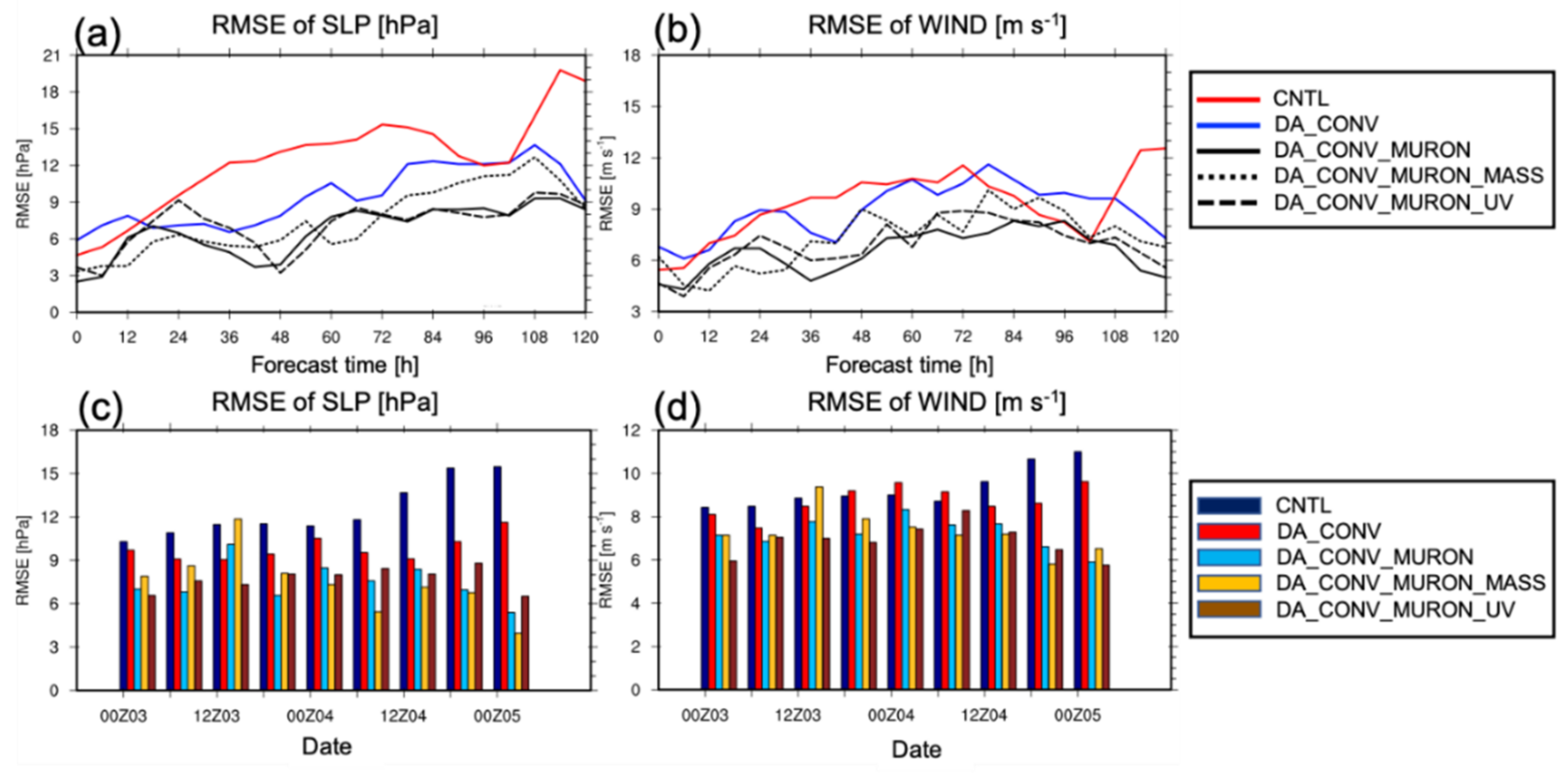
5.1. Impact of Assimilating MURON Observation on the Accuracy of the Analysis and Forecast

In this section, we evaluate the overall impact of the MURON observation on the analysis and subsequent forecast for all DA cycles. Figure 6 shows the RMS errors (RMSEs) of intensity forecasts averaged over all DA cycles (Figure 6a,b) and for each cycle (Figure 6c,d). In Figure 6c,d, the RMSEs of intensity forecasts are averaged over all the 00-h to 120-h lead times with a 6-h interval at each cycle. Compared to the control run, the RMSE of MSLP and wind speed forecasts of DA_CONV_MURON averaged over all cycles are reduced by 30.2% and 27.5% while the RMSE of the DA_CONV forecasts are reduced by 20.2% and 7.8%, respectively (Figure 6a,b). Assimilating both the conventional and MURON observations improves MSLP and wind speed forecasts for most DA cycles, with a more substantial RMSE reduction at later cycles as the control run, and the DA_CONV has diverged from the nature run at a later time (Figure 6c,d).
The vertical profiles of the RMSE of the control run and DA run analyses are shown in Figure 7. The RMSE is averaged within the 500 km radius from the TC center over all DA cycles. Assimilating the conventional observations reduces the wind and temperature analysis errors at almost all levels (Figure 7a,b). Assimilating MURON observations reduces the wind analysis error significantly below about 400 hPa compared to the conventional observations (Figure 7a). The temperature analysis error is reduced primarily at the lower levels below about 700 hPa compared to the DA_CONV analysis (Figure 7b). Figure 7c shows that assimilating conventional and MURON observations has a neutral impact on the mixing ratio analysis or even degrades the mixing ratio analysis from the surface to the middle level (600 hPa) compared to the control run. This result, in regard to the moisture variable, is unexpected because the surface moisture field and its spatial variability play a crucial role in the intensification of TCs [76], and the assimilation of such observed information should improve the analysis. Sensitivity tests that assimilated each MURON variable show that all observed variables except specific humidity increased the error of the surface mixing ratio analysis (not shown). This result therefore implies that the ensemble estimated cross-error correlation between the moisture variable and non-moisture variables observed by MURON is inaccurate. This issue will be discussed in Section 5.4 where the impact of selection of different moisture control variables is discussed.

5.2. Diagnostics of the Impact of MURON Observation on the RI Forecast

To further diagnose the impact of the assimilation of MURON observations on the RI forecast of Haiyan, the DA cycle initialized at 1800 UTC 3 November 2013 was analyzed. Typhoon Haiyan developed into a tropical storm and continued to intensify and began its RI at 0000 UTC 4 November 2013. This DA cycle is chosen because the 6-h forecast initialized by the DA_CONV_MURON analysis at 1800 UTC 3 November develops into the tropical storm while the control run does not (not shown in the figure). The cyclone valid at 1800 UTC 3 November is not well established in the control run (Figure 8b) and is mis-located in the DA_CONV analysis (Figure 8c). However, the DA_CONV_MURON analysis establishes a primary circulation with a position and an intensity more consistent with the nature run (Figure 8d). In addition, the DA_CONV_MURON analysis shows stronger winds to the north of the TC center and captures the asymmetric wind structure of the nature run (Figure 8d) which is commonly observed in TCs [77,78,79]. Assimilating the conventional and MURON observations increases the magnitude of the wind field below about 700 hPa to the north of the TC center (Figure 8h) while the DA_CONV analysis shows similar vertical structure of the wind with the control run (Figure 8f,g). Assimilating MURON leads to less tilt below 600 hPa, which is more consistent with the nature run (Figure 8e). However, MURON observations have a limited impact on the analysis at mid- to upper-levels above 400 hPa, where nature run shows strong upper-level flow (Figure 8e). In addition, assimilating MURON observations improves the pattern of the upward increase of the equivalent potential temperature (θe) near the TC center, which is consistent with structures of stronger TCs (Figure 8h). Although Figure 8 shows that the impacts of MURON are limited at the lower level below about 500 hPa, they affect the vertical tilting of wind and the vertical transport of moisture near the TC center which are favorable for TC intensification within the boundary layer [80].
Surface latent heat flux is a crucial factor determining the vertical extent of TC and plays an important role in TC formation and intensification [81]. Figure 9 shows that the DA_CONV_MURON analysis shows improvement in the spatial distribution and the magnitude of the surface latent heat flux compared to the control run and the DA_CONV analysis (Figure 9b,c). The MURON observations intensify the surface circulation, and the strong surface convergence causes a warm and moist surface air to rise above the ocean surface as shown by the upward increases of θe (Figure 8h). The DA_CONV_MURON run condenses and releases more latent heat near the inner core of the storm, which is more consistent with the nature run when compared to the control run.
Figure 10 shows the azimuthally averaged tangential wind, radial wind, and boundary layer height of the analyses valid at 1800 UTC 3 November. The nature run has a wind speed maximum within 40 km and 80 km from the TC center and between 200 m and 1000 m in altitude (Figure 10a), which is similar to that obtained from the composite analysis from past studies [82,83]. The tangential winds of the control run and the DA_CONV analysis are much weaker and the radius of maximum wind is much larger than the nature run (Figure 10b,c). In comparison, both the magnitude and the radius of maximum wind of DA_CONV_MURON are more consistent with the nature run (Figure 10d). In addition, assimilating MURON results in a stronger radial inflow at the lower level below about 1 km, which is more consistent with the nature run when compared to the control run.
The impact of MURON observations on boundary layer structure is evaluated by comparing boundary layer heights against the nature run. The boundary layer height for each column is defined as the level of the maximum wind speed following [83]. The boundary layer height has been identified to have a significant influence on TC intensification through controlling energy transport from the surface layer to the boundary layer above [16,84]. In the nature run, the boundary layer height increases from 10 km to 70 km, levels off between 80 km and 240 km, and increases beyond 250 km (Figure 10a). Assimilating MURON observations enhances the horizontal inflow and improves the vertical wind distribution (Figure 10d), resulting in a boundary layer height closer to the nature run when compared to the control run and the DA_CONV analysis (Figure 10b,d). These results imply that assimilating the MURON observations improves the analysis not only near the surface but also through the lower levels, affecting the TC intensification by regulating the energy transport process from the surface layer to the boundary layer above.
To investigate how the improved analysis leads to more accurate intensification forecast of Haiyan compared to the control run, the mass flux and vorticity are calculated within the TC inner region. The divergence term of the vorticity tendency equation depends on the absolute vorticity and divergence of the flow; therefore, the area averaged absolute vorticity (Figure 11a) and the area averaged vertical transport of mass flux (Figure 11b) are calculated for the analysis and 6-h forecast within 500 km from the TC center. The vertical mass flux is used to estimate the divergence of flow.
Assimilating conventional observations has little impact on the absolute vorticity analysis and the 6-h forecast compared to the control run (Figure 11a). On the other hand, the DA_CONV_MURON analysis has stronger absolute vorticity that is closer to the nature run than the control run and the DA_CONV analysis for all model levels at the initial time valid at 1800 UTC 3 November 2013 (Figure 11a). During the 6-h forecast, like the nature run, the vorticity of DA_CONV_MURON intensifies at almost every level, with its magnitude closer to the nature run than the control run and the DA_CONV forecast (Figure 11a). For the mass flux, the DA_CONV analysis is stronger than the control run below about 500 hPa and is weaker than the DA_CONV_MURON for all levels (Figure 11b). The DA_CONV_MURON analysis at the initial time is stronger than the control run for all levels (Figure 11b), matching closer to the nature run. Below 900 hPa, the DA_CONV_MURON analysis has nearly identical mass flux as the nature run. At the 6-h forecast time, the mass flux of the DA_CONV_MURON run increases, especially at the mid-levels between 700 hPa and 400 hPa, with its magnitude more consistent with the nature run and stronger than the control run (Figure 11b). Overall, the DA_CONV_MURON run has a stronger circulation at almost all levels with greater convergence at low to mid-levels in the analysis than the control run and the DA_CONV. This can contribute to a more rapid evolution of the vorticity than the control run in the subsequent forecast.
While near-ocean surface observations are assimilated, the DA_CONV_MURON analysis has larger vorticity (Figure 11) and higher moisture (Figure 8h) than the control run and the DA_CONV analysis from low to mid-levels below 500 hPa, which are integral for the development of deep convection [85,86]. As shown by the outgoing longwave radiation (OLR) in Figure 12, the DA_CONV_MURON run produces deep convection that is more consistent with the nature run than the control run and the DA_CONV. Specifically, the 6-h forecast of DA_CONV_MURON valid at 0000 UTC 04 shows deep convection cells organized near the TC center (Figure 12d) that are consistent in magnitude and distribution with the nature run than the control run and the DA_CONV (Figure 12). This result suggests that assimilating the MURON surface observation is able to induce vertical mixing to transport energy from the surface to the level above, which aids the development of deep convection. This result suggests that assimilating the MURON surface observations makes vortex stronger, which is a consistent convective structure with the nature run compared to the other.

5.3. Influence of MASS and WIND Observations of MURON

In this subsection, the impact of mass and wind observations from MURON are individually examined. Figure 6 shows that assimilating the conventional observations and the MURON wind observations (DA_CONV_MURON_WIND) improves the intensity forecast more than assimilating the conventional observations and the MURON mass observation (DA_CONV_MURON_MASS) at the early DA cycles before 0000 UTC 4 November 2013, when the simulated Haiyan is at the tropical disturbance (TD) stage (Figure 6c,d). This is likely because the assimilation of wind observations is more effective in correcting an initial TC vortex structure compared to that of mass observations [87]. However, during the later DA cycles after 0000 UTC 4 November 2013 when the simulated Haiyan has developed into a tropical storm (TS) stage followed by the RI, the assimilation of the MURON wind observations has a less positive impact than the assimilation of the MURON mass observations (Figure 6c,d). To investigate the potential source of the intensity forecast errors of DA_CONV_MURON_WIND during the TS stage, we examine the degree of physical balance between the mass and wind fields of the analysis and short-term forecasts. The maximum 10-m surface wind (VMAX) of the analysis, 6-h, 12-h, 18-h, and 24-h forecasts, are compared to the maximum 10-m surface wind (VMAXAH) which is derived from the pressure–wind relationship of [88]:
V M A X A H = 3.4 1010 M S L P 0.644
where MSLP is the minimum sea level pressure of the analysis, 6-h, 12-h, 18-h, and 24-h forecasts, and 1010 is a constant environmental pressure (hPa) valid for the Western North Pacific [89]. The equation was derived from an empirical relationship between the maximum surface wind and MSLP based on long-term observations. If the analysis and short-term forecasts maintain the balance between mass and wind fields, they should generally follow the relationship of Equation (5) in all the DA cycles. Figure 13 shows the scatter plot of VMAX (red dot) and VMAXAH (blue dot) as a function of MSLP from the TD (filled circle) and TS (open circle) stages of the DA cycles.
DA_CONV_MURON_WIND produces a larger imbalance between pressure and wind fields than DA_COVN_MURON_MASS, especially when the simulated Haiyan is at the TS stage (Figure 13). As the DA cycle continues, the imbalance between pressure and wind in DA_CONV_MURON_WIND accumulates, contributing to errors in the intensity forecast due to the generation of unrealistic inertia-gravity and its adjustment process during the model integration [90,91] (Figure 6c,d). The positive impact of mass observations during Haiyan’s TS stage demonstrates the potential advantage of the MURON observation platform which samples both wind and mass fields compared to the wind alone remote sensing platforms such as CYGNSS and SATWIND for TC forecasts. These results are consistent with a previous study that showed the benefit of assimilating surface pressure observations together with the wind observations for mesoscale convective system simulations [92].

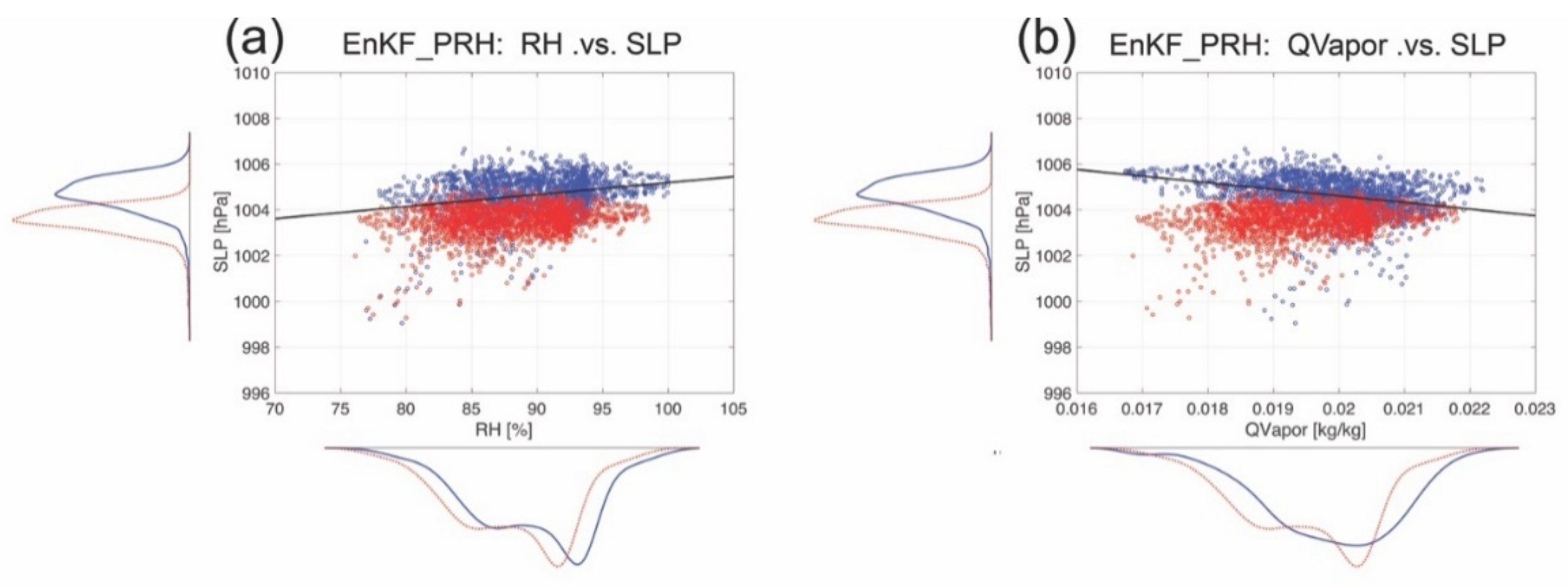
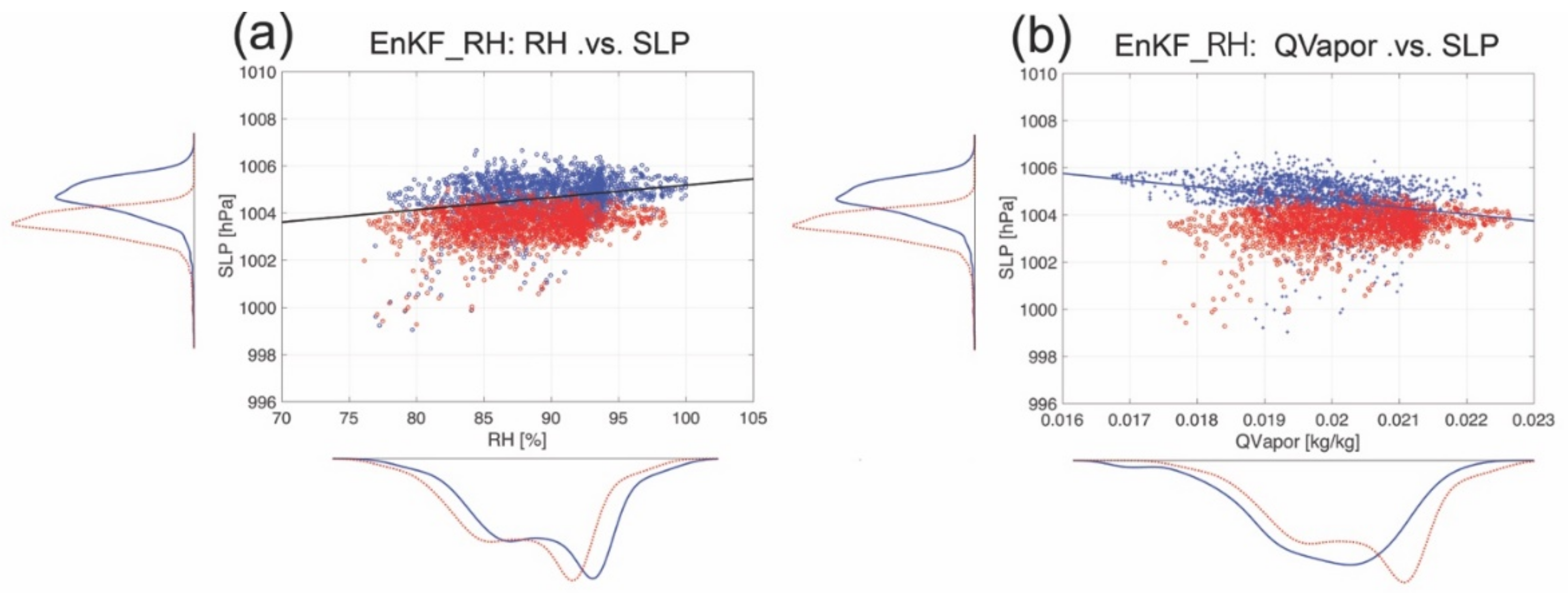
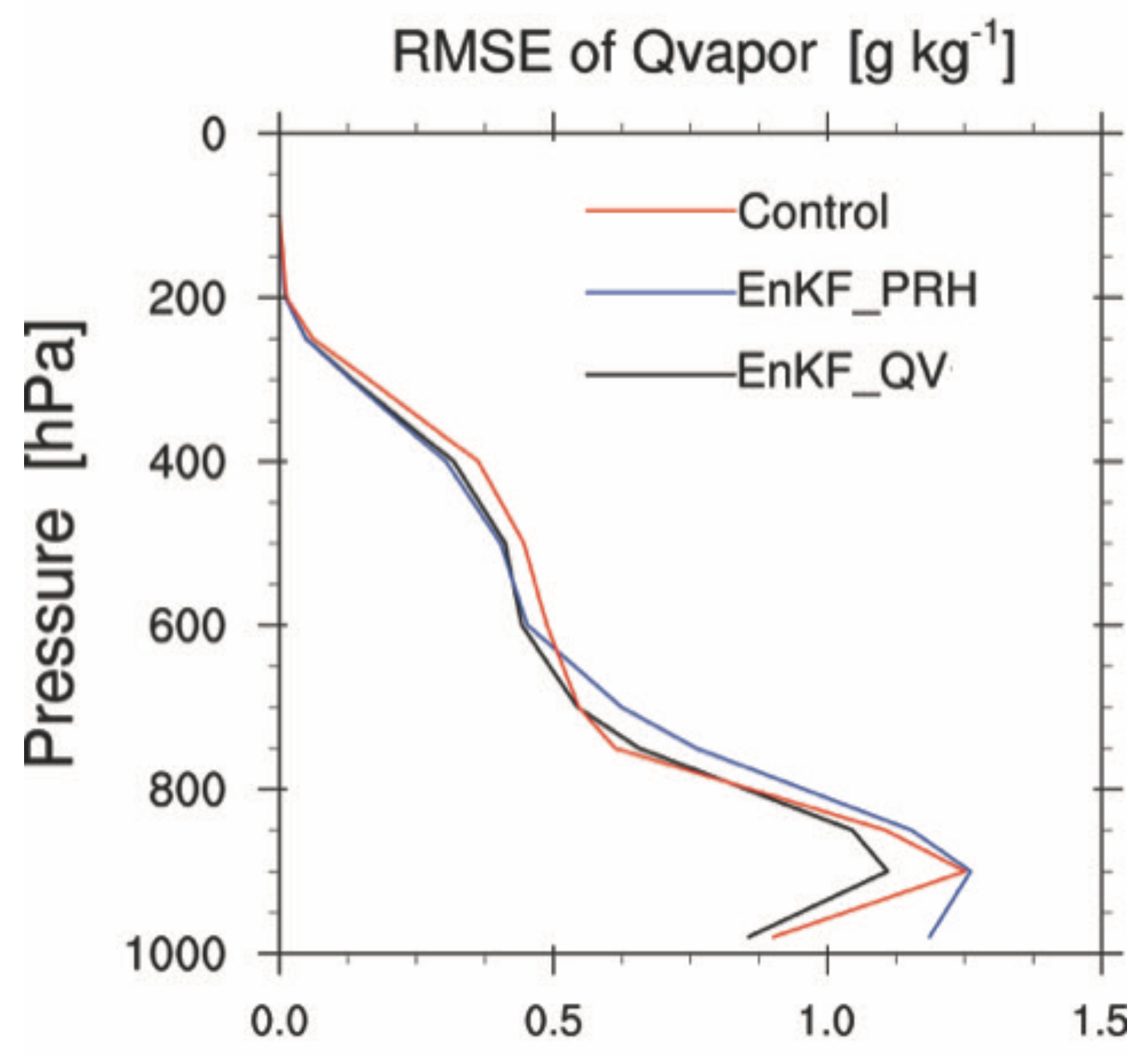
5.4. Impact of Moisture Control Variable

As discussed in Section 5.1, assimilating the conventional and MURON observations has a neutral or negative effect on the moisture analysis from the surface to mid-levels (Figure 7c). The degradation of the moisture analysis also occurs even when the non-moisture variables of the MURON observations are assimilated. Additional diagnostics to identify the cause are discussed in this section.
Pseudo RH (PRH) is the moisture control variable in the GSI EnKF DA system [51,52]. That is, a background ensemble PRH is updated by assimilating the MURON observations, as shown in Equations (1) and (2). The updated ensemble PRH from the DA is then converted to the WRF prognostic variable, water vapor mixing ratio, before being used to initialize the next WRF background forecast. Mathematically, the PRH ensemble member is defined as
P R H i = w i w ¯ s b = w i w ¯ s T ¯ b , p ¯ b ,
where w, p, and ws are the water vapor mixing ratio, pressure, and saturation mixing ratio, respectively. w ¯ s b is the saturation mixing ratio with respect to the background ensemble mean temperature ( T ¯ b ) and pressure ( p ¯ b ) where the overbar denotes the ensemble mean. Previous studies have shown that the PRH control variable can better fit background humidity to the observation in a global variational radiance DA system [93,94]; however, the impact of using PRH as the control variable in EnKF-based DA for TC forecasts remains to be explored.
To highlight the issues associated with using PRH as control variable and its transformation, we assume there is a central sea level pressure (SLP) observation that is available for assimilation. Figure 14 shows the DA_CONV_MURON 6-h background ensemble cross-correlation between the SLP at the TC center (marked by black dot) and the near surface water vapor mixing ratio, RH, and temperature throughout the domain valid at 1800 UTC 3 November 2013. Because the analysis ensemble mean mixing ratio has a large error northwest of the TC center (Figure 14d), this focused region (indicated by the black box) is selected for detailed diagnostics. The background SLP has a negative correlation with the background mixing ratio and temperature ensemble northwest of the TC center (indicated by the black box) (Figure 14a,b). This suggests that when the SLP observation innovation is negative, indicating a stronger observed TC, both the temperature and the mixing ratio are higher. This is consistent with known TC structure. On the other hand, the correlation of RH and SLP has the opposite sign. Because the elevated temperature increases the saturation mixing ratio (ws), RH will relatively decrease, despite the increase in the mixing ratio northwest of the TC center (Figure 14b).
To further reveal how using the PRH moisture control variable can lead to large moisture analysis error at the northwest of the TC center, a single SLP observation is assimilated at the TC center using the EnKF DA with the PRH moisture control variable valid at 1800 UTC 3 November 2013. Hereafter, we refer to this configuration as EnKF_PRH. Figure 15 shows the scatter plots and ensemble estimated probability density function (PDF) of the SLP (y-axis) and the surface moisture variable (x-axis) in the region enclosed in the black box. The red and blue colors represent the analysis ensemble and background ensemble, respectively. The SLP ensemble was sampled from 49 points around the TC center, so a total of 1960 samples (NS) represent the distribution. The same number (NS) of the ensemble of the moisture is sampled in the black box of Figure 14. By assimilating a single SLP observation of 1002 hPa, which has a lower value than the background ensemble mean of 1004.6 hPa, the background ensemble mean of both the SLP and PRH decrease because of the positive cross-correlation of the errors, as indicated by the blue scattered dots (Figure 15a). Figure 15b (red dots) shows the analysis ensemble mixing ratio that is converted from the updated ensemble PRH following Equation (6). The analysis ensemble mean mixing ratio shows a lower value (0.0195 kg kg−1) than the background ensemble mean (0.0199 kg kg−1). This result, however, conflicts with the correlation of SLP and mixing ratio collected from the background ensemble directly (Figure 15b blue dots). The background ensemble shows a negative cross-correlation between these two variables (Figure 15b blue dots). This negative correlation suggests that if the same SLP observation is assimilated, the mixing ratio should be corrected toward a larger value compared to the background. In other words, the mixing ratio will be adjusted toward the opposite direction when PRH is used as the control variable compared to when the mixing ratio is used as the control variable. This is because the background ensemble mean saturation mixing ratio ( w ¯ s b ) does not reflect the temperature change in the analysis when converting from the updated PRH to the mixing ratio according to Equation (6). To confirm this hypothesis, we conducted another experiment (EnKF_RH) where the analysis ensemble mixing ratio is generated by multiplying the updated ensemble RH with an analysis ensemble mean saturation mixing ratio ( w ¯ s ), not the background ensemble mean saturation mixing ratio ( w ¯ s b ). Figure 16b shows that with this configuration, the analysis ensemble mean mixing ratio (0.0203 kg kg−1) is larger than the background ensemble mean (0.0199 kg kg−1), which is consistent with the background ensemble estimated negative cross-correlation between the mixing ratio and SLP. Additional calculations shows that EnKF_RH analysis ensemble mean mixing ratio has a lower RMSE than EnKF_PRH (not shown). This is in contrast to earlier studies which revealed the advantage of using PRH for large scale DA [93,95]. In mesoscale applications, temperature and moisture fields have much larger variability in space and time. Our results suggest that the use of PRH as the moisture control variable in the EnKF DA may not update the temperature and mixing ratio consistently, which can lead to degradation of the moisture analysis.
It is also noted that the error distribution of the background ensemble PRH or RH is highly skewed and non-Gaussian. This deviation from Gaussianity is because RH has both a lower (0%) and an upper bound (100%) (Figure 16a). The non-Gaussian distribution of the background ensemble can produce a suboptimal analysis solution in the EnKF DA [96,97]. To evaluate the effect of a non-Gaussian error distribution of the background RH ensemble on the moisture analysis in the EnKF DA, we assimilate the same SLP observation used in Figure 15 using the Particle Filter (PF) DA method with the RH set as the moisture control variable (hereafter denoted as PF_RH). Because the PF method estimates the model probability densities conditioned on the observations without assuming the background ensemble error distribution [98,99], we expect that the PF DA method will produce a more realistic analysis distribution than the EnKF DA method. Note that PF_RH example presented here only assimilates one observation for demonstration purposes and no treatment on PF degeneration is implemented. The comparison between PF_RH and EnKF_RH reveals how the non-Gaussian error distribution of the background ensemble RH impacts the moisture analysis accuracy in the EnKF DA method.
Figure 17 shows the scatter plots similar to Figure 16, but with results from PF_RH. Although PF_RH and EnKF_RH have almost the same ensemble mean mixing ratio (0.0203 kg kg−1), the updated ensemble RH of PF_RH has a distinct PDF shape compared to that of EnkF_RH (Figure 16a vs. Figure 17a red curves). Such a distinct shape also shows up in the converted mixing ratio (Figure 16b vs. Figure 17b red curves). In the PF DA, assimilating the SLP observation further reduces the background ensemble RH near the maximum peak of the PDF (Figure 17a), while assimilating the SLP observation using the EnKF DA decreases the background ensemble mean RH while maintaining the overall shape of the background ensemble PDF (Figure 16a). This is because the EnKF aims to correct the background ensemble mean (Equation (1)) and to reduce the variance of the background ensemble perturbations (Equation (2)) using an assumption of the underlying Gaussian error distribution. The incorrect estimate of higher moments of the analysis distribution will lead to an incorrect subsequent first guess distribution, which accumulates as the forecast cycles.
Mixing ratio was used as an alternative moisture control variable in an experimental run (EnKF_QV) to examine its impact as a mitigation strategy for the aforementioned issue. Unlike RH or PRH, which have both upper and lower bounds, the background ensemble distribution of mixing ratio only has a lower bound and is closer to a Gaussian distribution (Figure 15a vs. Figure 15b, blue curves). The impact of assimilating MURON observations on the moisture analysis using PRH and QV as control variables is compared (Figure 18). The vertical profile of RMSEs is averaged over all DA cycles, as in Figure 7. The use of mixing ratio instead of PRH as the moisture control variable (EnKF_QV) leads to an improved mixing ratio analysis compared to the control run at lower levels below 800 hPa (Figure 18). Despite the positive impact shown here, preceding studies [93,94] suggest that mixing ratio and its error have a much larger spatiotemporal variability compared to RH, which can lead to errors in the global (non-mesoscale) moisture analysis and the subsequent global forecast. The results presented here indicate that future study is needed to identify the optimal selection of moisture variables for mesoscale DA.

6. Summary and Discussion

This research conducted an OSSE to estimate the effects of potential future new ocean surface MURON wind and mass observations on the RI forecasts using typhoon Haiyan as a case study. MURON consists of a high spatiotemporal resolution observation network, providing in-situ measurements of surface mass and wind fields over the West Pacific Ocean. It is expected that MURON can provide lower-level information near the TC inner core, where the energy flux transfer from the ocean surface plays a critical role for the RI process in TCs. It is found that assimilating the MURON observation together with the conventional observations reduces the TC intensity forecast error by about 30% and 10~20% compared to the control run and the DA_CONV when averaged over all DA cycles. While assimilating conventional observations has a marginal or neutral impact on the analysis compared to the control run, assimilating the MURON observations improves the structure and magnitude of near-surface analyzed fields, including SLP, wind, temperature, moisture, latent heat flux, and PBL height. The improvement of surface analysis fields affects subsequent forecasts from the surface to the middle levels by correcting the initial vorticity and vertical mass flux. These favorable conditions for moist convection in the TC inner core improve the RI forecast and reduce TC intensity forecast errors when compared against the control run and the DA_CONV.
MURON wind and mass observations show distinct effects on the TC intensity forecast during the TD and TS stages of typhoon Haiyan. Assimilating the MURON wind observations reduces the intensity forecast error more than the MURON mass observations at the TD stage through correcting the initial vortex structure efficiently. However, the MURON wind observations cause an imbalance between the wind and pressure fields of the analysis especially, during the TS stage, which reduces its positive impact on the intensity forecast at the TS stage. Compared to the MURON wind observations, the assimilation of the MURON mass observations is less effective in reinforcing the circulation when the inner core structure of typhoon Haiyan is not well developed before the beginning of the RI. However, the assimilation of the MURON mass observations reduces intensity forecast errors more than the MURON wind observations after the onset of the RI process because the mass observations maintain a better balance between the wind and pressure fields of the analysis than wind observations.
The impact of assimilating the MURON observations on the moisture analysis is dependent on the selection of the moisture control for the EnKF update. A neutral or negative impact on the low-level moisture analysis is found when PRH is used as a moisture control variable. This problem is caused by two factors: (1) the updated temperature field is not considered in the nonlinear conversion from the updated PRH moisture control variable to the mixing ratio analysis, and (2) the EnKF can generate a suboptimal moisture analysis error distribution due to the non-Gaussian distribution of the background ensemble PRH, which happens more frequently in a humid environment. The use of mixing ratio as the control variable avoids or alleviates these issues and improves the moisture analyses using the MURON observations.
This study is the first to explore the potential impact of the future ocean surface observations from MURON on the TC intensity forecasts. This initial study is limited by the exploration of a single TC case. Further studies are planned to address how the MURON observation complements other existing observations for TC forecasts.

Author Contributions

Conceptualization, J.K. and X.W.; methodology, J.K. and X.W.; investigation, J.K. and X.W.; data preparation, J.K. and M.Y.; validation, J.K. and X.W.; draft writing, J.K.; review and revise, X.W. and M.Y.; supervision, X.W. All authors have read and agreed to the published version of the manuscript.

Funding

This research was funded by WNI grants 17-FY15-ORA3-41 and 24-FY18-ORA5-8.

Institutional Review Board Statement

Not applicable.

Informed Consent Statement

Not applicable.

Data Availability Statement

Not applicable.

Acknowledgments

The authors acknowledge Bob Palmer and Yan Zhang for initial discussion. Some results were presented at the AMS annual meeting.

Conflicts of Interest

The authors declare no conflict of interest.

References

  1. Lawrence, M.B.; National Hurricane Center Verification. NOAA. 1990. Available online: www.nhc.noaa.gov/verification/verify3.shtml (accessed on 30 March 2022).
  2. McAdie, C.J.; Lawrence, M.B. Improvements to tropical cyclone track forecasting in the Atlantic basin, 1970–98. Bull. Am. Meteorol. Soc. 2000, 81, 989–998. [Google Scholar] [CrossRef]
  3. Cangialosi, J.P. 2018 Hurricane Season. National Hurricane Center Forecast Verification Report. 2019. Available online: https://www.nhc.noaa.gov/verification/pdfs/Verification_2018.pdf (accessed on 30 March 2022).
  4. Rappaport, E.N.; Franklin, J.L.; Avila, L.A.; Baig, S.R.; Beven II, J.L.; Blake, E.S.; Burr, C.A.; Jiing, J.-G.; Juckins, C.A.; Knabb, R.D. Advances and challenges at the National Hurricane Center. Weather Forecast. 2009, 24, 395–419. [Google Scholar] [CrossRef] [Green Version]
  5. Cangialosi, J.P.; Franklin, J.L. National Hurricane Center Verification Report; Tropical Prediction Center, National Hurricane Center, National Center for Environmental Prediction, National Weather Center, NOAA: Miami, FL, USA, 2006; p. 57.
  6. Emanuel, K.A. Thermodynamic control of hurricane intensity. Nature 1999, 401, 665–669. [Google Scholar] [CrossRef]
  7. Zhang, F.; Sippel, J.A. Effects of moist convection on hurricane predictability. J. Atmos. Sci 2009, 66, 1944–1961. [Google Scholar] [CrossRef]
  8. Fang, J.; Zhang, F. Initial development and genesis of hurricane Dolly (2008). J. Atmos. Sci. 2010, 67, 655–672. [Google Scholar] [CrossRef]
  9. Fang, J.; Zhang, F. Evolution of multi-scale vortices in the development of Hurricane Dolly (2008). J. Atmos. Sci. 2011, 68, 103–122. [Google Scholar] [CrossRef] [Green Version]
  10. Taraphdar, S.; Mukhopadhyay, P.; Leung, L.R.; Zhang, F.; Abhilash, S.S.; Goswami, B.N. The role of moist processes in the intrinsic predictability of Indian Ocean cyclones. J. Geophys. Res. Atmos. 2014, 119, 8032–8048. [Google Scholar] [CrossRef]
  11. Bender, M.A.; Ginis, I.; Tuleya, R.; Thomas, B.; Marchok, T. The operational GFDL hurricane–ocean prediction system and a summary of its performance. Mon. Weather Rev. 2007, 135, 3965–3989. [Google Scholar] [CrossRef]
  12. Davis, C.; Wang, W.; Chen, S.S.; Chen, Y.; Corbosiero, K.; DeMaria, M.; Dudhia, J.; Holland, G.; Klemp, J.; Michalakes, J.; et al. Prediction of landfalling hurricanes with the Advanced Hurricane WRF model. Mon. Weather Rev. 2008, 136, 1990–2005. [Google Scholar] [CrossRef] [Green Version]
  13. Zhang, F.; Tao, D. Effects of vertical wind shear on the predictability of tropical cyclones. J. Atmos. Sci. 2013, 70, 975–983. [Google Scholar] [CrossRef]
  14. Black, P.G.; D’Asaro, E.A.; Drennan, W.M.; French, J.R.; Niiler, P.P.; Sanford, T.B.; Terrill, E.J.; Walsh, E.J.; Zhang, J.A. Air-sea exchange in hurricanes: Synthesis of observations from the Coupled Boundary Layer Air–Sea Transfer experiment. Bull. Am. Meteorol. Soc. 2007, 88, 357–374. [Google Scholar] [CrossRef] [Green Version]
  15. Price, J.F. Metrics of hurricane–ocean interaction: Vertically-integrated or vertically-averaged ocean temperature? Ocean Sci. 2009, 5, 351–368. [Google Scholar] [CrossRef] [Green Version]
  16. Zhang, J.A. Estimation of dissipative heating using low-level in situ aircraft observations in the hurricane boundary layer. J. Atmos. Sci. 2010, 67, 1853–1862. [Google Scholar] [CrossRef] [Green Version]
  17. Kepert, J.D. Choosing a boundary layer parameterization for tropical cyclone modeling. Mon. Weather Rev. 2012, 140, 1427–1445. [Google Scholar] [CrossRef] [Green Version]
  18. Green, B.W.; Zhang, F. Impacts of air–sea flux parameterizations on the intensity and structure of tropical cyclones. Mon. Weather Rev. 2013, 141, 2308–2324. [Google Scholar] [CrossRef] [Green Version]
  19. Ricchi, A.; Miglietta, M.M.; Barbariol, F.; Benetazzo, A.; Bergamasco, A.; Bonaldo, D.; Cassardo, C.; Falcieri, F.M.; Modugno, G.; Russo, A.; et al. Sensitivity of a Mediterranean Tropical-Like Cyclone to Different Model Configurations and Coupling Strategies. Atmosphere 2017, 8, 92. [Google Scholar] [CrossRef] [Green Version]
  20. Nguyen, V.S.; Smith, R.K.; Montgomery, M.T. Tropical-cyclone intensification and predictability in three dimensions. Q. J. R. Meteorol. Soc. 2008, 134, 563–582. [Google Scholar]
  21. Wang, H.; Wang., Y. A numerical study of Typhoon Megi (2010). Part I: Rapid intensification. Mon. Weather Rev. 2014, 142, 29–48. [Google Scholar] [CrossRef]
  22. Emanuel, K.; DesAutels, C.; Holloway, C.; Korty, R. Environmental control of tropical cyclone intensity. J. Atmos. Sci. 2004, 61, 843–858. [Google Scholar] [CrossRef]
  23. Zou, X.; Qin, Z.; Weng, F. Improved coastal precipitation forecasts with direct assimilation of GOES-11/12 imager radiances. Mon. Weather Rev. 2011, 139, 3711–3729. [Google Scholar] [CrossRef] [Green Version]
  24. Zou, X.; Qin, Z.; Zheng, Y. Improved tropical storm forecasts with GOES-13/15 imager radiance assimilation and asymmetric vortex initialization in HWRF. Mon. Weather Rev. 2015, 143, 2485–2505. [Google Scholar] [CrossRef]
  25. Chelton, D.B.; Freilich, M.H.; Sienkiewicz, J.M.; von Ahn, J.M. 2006: On the use of QuikSCAT Scatterometer measurements of surface winds for marine weather prediction. Mon. Weather Rev. 2006, 134, 2055–2071. [Google Scholar] [CrossRef]
  26. Brennan, M.J.; Hennon, C.C.; Knabb, R.D. The operational use of QuikSCAT ocean surface vector winds at the National Hurricane Center. Weather Forecast. 2009, 24, 621–645. [Google Scholar] [CrossRef] [Green Version]
  27. Desbiolles, F.; Bentamy, A.; Blanke, B.; Roy, C.; Mestas-Nuñez, A.M.; Grodsky, S.A.; Herbette, S.; Cambon, G.; Maes, C. Two decades (1992–2012) of surface wind analyses based on satellite scatterometer observations. J. Mar. Syst. 2017, 168, 38–56. [Google Scholar] [CrossRef] [Green Version]
  28. Ruf, C.S.; Atlas, R.; Chang, P.S.; Clarizia, M.P.; Garrison, J.L.; Gleason, S.; Katzberg, S.J.; Jelenak, Z.; Johnson, J.T.; Majumdar, S.J.; et al. New ocean winds satellite mission to probe hurricanes and tropical convection. Bull. Am. Meteorol. Soc. 2016, 97, 385–395. [Google Scholar] [CrossRef]
  29. Zhang, S.; Pu, Z.; Posselt, D.J.; Atlas, R. Impact of CYGNSS ocean surface wind speeds on numerical simulations of a hurricane in observing system simulation experiments. J. Atmos. Ocean. Technol. 2017, 34, 375–383. [Google Scholar] [CrossRef]
  30. Ruf, C.S.; Chew, C.; Lang, T.; Morris, M.G.; Nave, K.; Ridley, A.; Balasubramaniam, R. New paradigm in Earth environmental monitoring with the CYGNSS small satellite constellation. Sci. Rep. 2018, 8, 8782. [Google Scholar] [CrossRef] [Green Version]
  31. Masutani, M.; Andersson, E.; Terry, J.; Reale, O.; Jusem, J.C.; Riishojgaard, L.P.; Schlatter, T.; Stoffelen, A.; Woollen, J.; Lord, S.; et al. Progress in Joint OSSEs: A new nature run and international collaboration. In Proceedings of the 12th Conference on Integrated Observing and Assimilation Systems for Atmospheres, Oceans, and Land Surface (IOAS-AOLS), New Orleans, LA, USA, 20–24 January 2008; Available online: http://ams.confex.com/ams/pdfpapers/124080.pdf (accessed on 30 March 2022).
  32. Masutani, M.; Woollen, J.S.; Lord, S.J.; Emmitt, G.D.; Kleespies, T.J.; Wood, S.A.; Greco, S.; Sun, H.; Terry, J.; Kapoor, V.; et al. Observing system simulation experiments at the National Centers for Environmental Prediction. J. Geophys. Res. 2010, 115, D07101. [Google Scholar] [CrossRef] [Green Version]
  33. Shu, S.; Zhang, F. Influence of equatorial waves on the genesis of Super Typhoon Haiyan (2013). J. Atmos. Sci. 2015, 72, 4591–4613. [Google Scholar] [CrossRef] [Green Version]
  34. Evans, A.D.; Falvey, R.J. Annual Joint Typhoon Warning Center Tropical Cyclone Report; JTWC: Hancock County, MI, USA, 2013; p. 118. [Google Scholar]
  35. Chen, Z.; Zhang, C.; Huang, Y.; Feng, Y.; Zhong, S.; Dai, G.; Xu, D.; Yang, Z. Track of Super Typhoon Haiyan predicted by a typhoon model for the South China Sea. J. Meteorol. Res. 2014, 28, 510–523. [Google Scholar] [CrossRef]
  36. Lander, M.; Guard, C.; Camargo, S.J. Tropical cyclones, super-typhoon Haiyan, in State of the Climate in 2013. Bull. Am. Meteorol. Soc. 2014, 95, S112–S114. [Google Scholar]
  37. Lin, I.-I.; Pun, I.-F.; Lien, C.-C. “Category-6” supertyphoon Haiyan in global warming hiatus: Contribution from subsurface ocean warming. Geophys. Res. Lett. 2014, 41, 8547–8553. [Google Scholar] [CrossRef]
  38. Huang, H.-C.; Boucharel, J.; Lin, I.-I.; Jin, F.-F.; Lien, C.-C.; Pun, I.-F. Air-sea fluxes for Hurricane Patricia (2015): Comparison with supertyphoon Haiyan (2013) and under different ENSO conditions. J. Geophys. Res. Oceans 2017, 122, 6076–6089. [Google Scholar] [CrossRef]
  39. Skamarock, W.C.; Klemp, J.B.; Dudhia, J.; Gill, D.O.; Barker, D.; Duda, M.G.; Huang, X.-Y.; Wang, W.; Powers, J.G. 2008: A Description of the Advanced Research WRF Version 3; NCAR Tech. Note, NCAR/TN-4751STR; NCAR: Boulder, CO, USA, 2008; p. 113. [Google Scholar] [CrossRef]
  40. Lim, K.S.; Hong, S. Development of an Effective Double-Moment Cloud Microphysics Scheme with Prognostic Cloud Condensation Nuclei (CCN) for Weather and Climate Models. Mon. Weather Rev. 2010, 138, 1587–1612. [Google Scholar] [CrossRef] [Green Version]
  41. Kain, J.S.; Fritsch, J.M. A one-dimensional entraining/detraining plume model and its application in convective parameterization. J. Atmos. Sci. 1990, 47, 2784–2802. [Google Scholar] [CrossRef] [Green Version]
  42. Kain, J.S. The Kain–Fritsch convective parameterization: An update. J. Appl. Meteorol. 2004, 43, 170–181. [Google Scholar] [CrossRef] [Green Version]
  43. Hong, S.-Y.; Noh, Y.; Dudhia, J. A new vertical diffusion package with an explicit treatment of entrainment processes. Mon. Weather Rev. 2006, 134, 2318–2341. [Google Scholar] [CrossRef] [Green Version]
  44. Hong, S.-Y. A new stable boundary layer mixing scheme and its impact on the simulated East Asian summer monsoon. Q. J. R. Meteorol. Soc. 2010, 136, 1481–1496. [Google Scholar] [CrossRef]
  45. Chen, F.; Dudhia, J. Coupling an advanced land surface–hydrology model with the Penn State–NCAR MM5 modeling system. Part I: Model implementation and sensitivity. Mon. Weather Rev. 2001, 129, 569–585. [Google Scholar] [CrossRef] [Green Version]
  46. Mlawer, E.J.; Taubman, S.J.; Brown, P.D.; Iacono, M.J.; Clough, S.A. Radiative transfer for inhomogeneous atmospheres: RRTM, a validated correlated-k model for the longwave. J. Geophys. Res. 1997, 102, 16663–16682. [Google Scholar] [CrossRef] [Green Version]
  47. Iacono, M.J.; Delamere, J.S.; Mlawer, E.J.; Shephard, M.W.; Clough, S.A.; Collins, W.D. Radiative forcing by long-lived greenhouse gases: Calculations with the AER radiative transfer models. J. Geophys. Res. 2008, 113, D13103. [Google Scholar] [CrossRef]
  48. Nolan, D.S.; Zhang, J.A.; Stern, D.P. Evaluation of planetary boundary layer parameterizations in tropical cyclones by comparison of in situ observations and high-resolution simulations of Hurricane Isabel (2003), Part I: Initialization, maximum winds, and the outer-core boundary layer. Mon. Weather Rev. 2009, 137, 3651–3674. [Google Scholar] [CrossRef]
  49. Nolan, D.S.; Atlas, R.; Bhatia, K.T.; Bucci, L.R. Development and validation of a hurricane nature run using the Joint OSSE nature run and the WRF model. J. Adv. Earth Model. Syst. 2013, 5, 382–405. [Google Scholar] [CrossRef]
  50. Stauffer, D.R.; Seaman, N.L. Use of four-dimensional data assimilation in a limited-area mesoscale model, Part I: Experiments with synoptic-scale data. Mon. Weather Rev. 1990, 118, 1250–1277. [Google Scholar] [CrossRef] [Green Version]
  51. Shao, H.; Derber, J.; Huang, X.Y.; Hu, M.; Newman, K.; Stark, D.; Lueken, M.; Zhou, C.; Nance, L.; Kuo, Y.H.; et al. Bridging research to operations transitions: Status and plans of community GSI. Bull. Am. Meteorol. Soc. 2016, 97, 1427–1440. [Google Scholar] [CrossRef]
  52. Hu, M.; Ge, G.; Zhou, C.; Stark, D.; Shao, H.; Newman, K.; Beck, J.; Zhang, X. Grid-Point Statistical Interpolation (GSI) User’s Guide Version 3.7. Developmental Testbed Center; p. 147. Available online: http://www.dtcenter.org/com-GSI/users/docs/index.php (accessed on 30 March 2022).
  53. Degelia, S.K.; Wang, X.; Stnsrud, D.J. An evaluation of the impact of assimilating AERI retrievals, kinematic profilers, rawinsondes, and surface observations on a forecast of a nocturnal convection initiation event during the PECAN field campaign. Mon. Weather Rev. 2019, 147, 2739–2764. [Google Scholar] [CrossRef]
  54. Smith, R.K. The role of cumulus convection in hurricanes and its representation in hurricane models. Rev. Geophys. 2000, 38, 465–489. [Google Scholar] [CrossRef]
  55. Nasrollahi, N.; AghaKouchak, A.; Li, J.; Gao, X.; Hsu, K.; Sorooshian, S. Assessing the impacts of different WRF precipitation physics in hurricane simulations. Weather Forecast. 2012, 27, 1003–1016. [Google Scholar] [CrossRef]
  56. Biswas, M.K.; Bernardet, L.; Dudhia, J. Sensitivity of hurricane forecasts to cumulus parameterizations in the HWRF model. Geophys. Res. Lett. 2014, 41, 9113–9119. [Google Scholar] [CrossRef]
  57. Mellor, G.L.; Yamada, T. Development of a turbulence closure model for geophysical fluid problems. Rev. Geophys. 1982, 20, 851–875. [Google Scholar] [CrossRef] [Green Version]
  58. Janjic, Z.I. The step-mountain coordinate: Physical package. Mon. Wea. Rev. 1990, 118, 1429–1443. [Google Scholar] [CrossRef]
  59. Janjic, Z.I. The step-mountain Eta coordinate model: Further developments of the convection, viscous layer, and turbulence closure schemes. Mon. Wea. Rev. 1994, 122, 927–945. [Google Scholar] [CrossRef] [Green Version]
  60. Janjic, Z.I. Nonsingular Implementation of the Mellor-Yamada Level 2.5 Scheme in the NCEP Meso Model; NOAA/NWS/NCEP Office Note 437; NOAA Science Center: Silver Spring, MD, USA, 2001; p. 61.
  61. Whitaker, J.S.; Hamill, T.M. Ensemble data assimilation without perturbed observations. Mon. Weather Rev. 2002, 130, 1913–1924. [Google Scholar] [CrossRef]
  62. Wu, C.; Lien, G.; Chen, J.; Zhang, F. Assimilation of tropical cyclone track and structure based on the Ensemble Kalman Filter (EnKF). J. Atmos. Sci. 2010, 67, 3806–3822. [Google Scholar] [CrossRef]
  63. Meng, Z.; Zhang, F. Limited-area ensemble-based data assimilation. Mon. Weather Rev. 2011, 139, 2025–2045. [Google Scholar] [CrossRef] [Green Version]
  64. Jung, B.-J.; Kim, H.M.; Zhang, F.; Wu, C.-C. Effect of targeted dropsonde observations and best track data on the track forecasts of Typhoon Sinlaku (2008) using an ensemble Kalman filter. Tellus A 2012, 64, 14984. [Google Scholar] [CrossRef]
  65. Lu, X.; Wang, X.; Tong, M.; Tallapragada, V. GSI-based, continuously cycled, dual-resolution hybrid ensemble-variational data assimilation system for HWRF: System description and experiments with Edouard (2014). Mon. Weather Rev. 2017, 145, 4877–4898. [Google Scholar] [CrossRef]
  66. Lu, X.; Wang, X.; Li, Y.; Tong, M.; Ma, X. GSI-based ensemble-variational hybrid data assimilation for HWRF for hurricane initialization and prediction: Impact of various error covariances for airborne radar observation assimilation. Q. J. R. Meteorol. Soc. 2017, 143, 223–239. [Google Scholar] [CrossRef]
  67. Wang, X.; Parrish, D.; Kleist, D.; Whitaker, J. GSI 3DVar-based ensemble–variational hybrid data assimilation for NCEP Global Forecast System: Single-resolution experiments. Mon. Weather Rev. 2013, 141, 4098–4117. [Google Scholar] [CrossRef]
  68. Wang, X.; Lei, T. GSI-based four-dimensional ensemble–variational (4DEnsVar) data assimilation: Formulation and single-resolution experiments with real data for NCEP Global Forecast System. Mon. Weather Rev. 2014, 142, 3303–3325. [Google Scholar] [CrossRef]
  69. Gaspari, G.; Cohn, S.E. Construction of correlation functions in two and three dimensions. Q. J. R. Meteorol. Soc. 1999, 125, 723–757. [Google Scholar] [CrossRef]
  70. Anderson, J.L.; Anderson, S.L. A Monte Carlo implementation of the nonlinear filtering problem to produce ensemble assimilations and forecasts. Mon. Weather Rev. 1999, 127, 2741–2758. [Google Scholar] [CrossRef]
  71. Whitaker, J.S.; Hamill, T.M. Evaluating methods to account for system errors in ensemble data assimilation. Mon. Weather Rev. 2012, 140, 3078–3089. [Google Scholar] [CrossRef]
  72. Torn, R.D.; Hakim, G.J.; Snyder, C. Boundary conditions for limited area ensemble Kalman filters. Mon. Weather Rev. 2006, 134, 2490–2502. [Google Scholar] [CrossRef]
  73. Wang, X.; Barker, D.M.; Snyder, C.; Hamill, T.M. A hybrid ETKF–3DVAR data assimilation scheme for the WRF model. Part I: Observing system simulation experiment. Mon. Weather Rev. 2008, 136, 5116–5131. [Google Scholar] [CrossRef] [Green Version]
  74. Desroziers, G.; Berre, L.; Chapnik, B.; Poli, P. Diagnosis of observation, background and analysis-error statistics in observation space. Q. J. R. Meteorol. Soc. 2005, 131, 3385–3396. [Google Scholar] [CrossRef]
  75. Wang, X.; Bishop, C.H. A comparison of breeding and en-semble transform Kalman filter ensemble forecast schemes. J. Atmos. Sci. 2003, 60, 1140–1158. [Google Scholar] [CrossRef]
  76. Cione, J.J.; Black, P.G.; Houston, S.H. Surface observations in the hurricane environment. Mon. Weather Rev. 2000, 128, 1550–1561. [Google Scholar] [CrossRef]
  77. Shapiro, L.J. The asymmetric boundary layer flow under a translating hurricane. J. Atmos. Sci. 1983, 40, 1984–1998. [Google Scholar] [CrossRef] [Green Version]
  78. Kepert, J.D. Observed boundary layer wind structure and balance in the hurricane core. Part I: Hurricane Georges. J. Atmos. Sci. 2006, 63, 2169–2193. [Google Scholar] [CrossRef]
  79. Schwendike, J.; Kepert, J.D. The boundary layer winds in Hurricane Danielle (1998) and Isabel (2003). Mon. Weather Rev. 2008, 136, 3168–3191. [Google Scholar] [CrossRef]
  80. DeMaria, M. The effect of vertical shear on tropical cyclone intensity change. J. Atmos. Sci. 1996, 53, 2076–2088. [Google Scholar] [CrossRef] [Green Version]
  81. Chen, S.S.; Price, J.F.; Zhao, W.; Donelan, M.A.; Walsh, E.J. The CBLAST-Hurricane program and the next generation fully coupled atmosphere–wave–ocean models for hurricane research and prediction. Bull. Am. Meteorol. Soc. 2007, 88, 311–317. [Google Scholar] [CrossRef]
  82. Franklin, J.L.; Black, M.L.; Valde, K. GPS dropwindsonde wind profiles in hurricanes and their operational implications. Weather Forecast. 2003, 18, 32–44. [Google Scholar] [CrossRef]
  83. Zhang, J.A.; Rogers, R.F.; Nolan, D.S.; Marks, F.D. On the characteristic height scales of the hurricane boundary layer. Mon. Weather Rev. 2011, 139, 2523–2535. [Google Scholar] [CrossRef]
  84. Wroe, D.R.; Barnes, G.M. Inflow layer energetics of Hurricane Bonnie (1998) near landfall. Mon. Weather Rev. 2003, 131, 1600–1612. [Google Scholar] [CrossRef]
  85. Gray, W.M. Global view of the origin of tropical disturbances and storms. Mon. Weather Rev. 1968, 96, 669–700. [Google Scholar] [CrossRef]
  86. Houze, R.A.; Lee, W.; Bell, M.M. Convective contribution to the genesis of Hurricane Ophelia (2005). Mon. Weather Rev. 2009, 137, 2778–2800. [Google Scholar] [CrossRef]
  87. Wu, C.; Chou, K.; Wang, Y.; Kuo, Y. Tropical cyclone initialization and prediction based on four-dimensional variational data assimilation. J. Atmos. Sci. 2006, 63, 2383–2395. [Google Scholar] [CrossRef]
  88. Atkinson, G.D.; Holliday, C.R. Tropical cyclone minimum sea level pressure-maximum sustained wind relationship for western North Pacific. Mon. Weather Rev. 1977, 105, 421–427. [Google Scholar] [CrossRef] [Green Version]
  89. Holland, G. A revised hurricane pressure–wind model. Mon. Weather Rev. 2008, 136, 3432–3445. [Google Scholar] [CrossRef] [Green Version]
  90. Kleist, D.T.; Parrish, D.F.; Derber, J.C.; Treadon, R.; Errico, R.M.; Yang, R. Improving incremental balance in the GSI 3DVAR analysis system. Mon. Weather Rev. 2009, 137, 1046–1060. [Google Scholar] [CrossRef]
  91. Piccolo, C. Growth of forecast errors from covariances modeled by 4DVAR and ETKF methods. Mon. Weather Rev. 2011, 139, 1505–1518. [Google Scholar] [CrossRef]
  92. Wheatley, D.M.; Stensrud, D.J. The impact of assimilating surface pressure observations on severe weather events in a WRF mesoscale ensemble system. Mon. Weather Rev. 2010, 138, 1673–1694. [Google Scholar] [CrossRef]
  93. Dee, D.P.; da Silva, A.M. The choice of variable for atmospheric moisture analysis. Mon. Weather Rev. 2003, 131, 155–171. [Google Scholar] [CrossRef] [Green Version]
  94. Gustafsson, N.; Thorsteinsson, S.; Stengel, M.; Holm, E. Use of a nonlinear pseudo-relative humidity variable in a multivariate formulation of moisture analysis. Q. J. R. Meteorol. Soc. 2011, 137, 1004–1018. [Google Scholar] [CrossRef]
  95. Takacs, L.L.; Suárez, M.J.; Todling, R. Maintaining atmospheric mass and water balance in reanalyses. Quart. J. Q. J. R. Meteorol. Soc. 2016, 142, 1565–1573. [Google Scholar] [CrossRef] [Green Version]
  96. Yang, S.; Kalnay, E.; Hunt, B. Handling nonlinearity in an ensemble Kalman filter: Experiments with the three-variable Lorenz model. Mon. Weather Rev. 2012, 140, 2628–2646. [Google Scholar] [CrossRef]
  97. Bishop, C.H. The GIGG–EnKF: Ensemble Kalman filtering for highly skewed non-negative uncertainty distributions. Q. J. R. Meteorol. Soc. 2016, 142, 1395–1412. [Google Scholar] [CrossRef]
  98. Snyder, C.; Bengtsson, T.; Morzfeld, M. Performance bounds for particle filters using optimal proposal. Mon. Weather Rev. 2015, 143, 4750–4761. [Google Scholar] [CrossRef]
  99. Van Leeuwen, P.J. Particle filtering in geophysical systems. Mon. Weather Rev. 2009, 137, 4089–4114. [Google Scholar] [CrossRef]
Figure 1. First generation of MURON instrument prototype designed by the intelligent aerospace radio team at the University of Oklahoma.
Atmosphere 13 00779 g001
Figure 2. Triply nested model domains with 361 × 221 grid points in the 27-km resolution domain (D01), 763 × 421 grid points in the 9 km domain (D2), and 1420 × 922 grid points in the 3 km domain (D3) and MURON float distribution (black dots) for innermost domain (D03).
Atmosphere 13 00779 g002
Figure 3. Schematic illustration of the DA procedures by GSI-based EnKF used in this study. Simulated conventional observations and MURON observations drawn from the nature run are assimilated in DA cycles.
Atmosphere 13 00779 g003
Figure 4. Comparison of (a) MSLP, (b) maximum surface wind speed, and (c) track among the JMA typhoon center best-track data (solid line), nature run (dotted line), and control run (dashed line). The color of dot represents each stage of the storm; tropical disturbance (TD; green), tropical storm (TS; blue), Saffir–Simpson category 1 (C1; yellow), category 2 (C2; orange), category 3 (C3; brown), and category 4 (C4; purple).
Atmosphere 13 00779 g004
Figure 5. A time series of RMS of innovation (solid line) and total spread (dotted line) for (a) surface pressure, (b) surface wind, (c) surface temperature, (d) surface specific humidity for GSI ocean surface observation error (GSI_R) (red line) and modified MURON observation error (MURON_R) (black line).
Atmosphere 13 00779 g005
Figure 6. The RMSEs of (a) MSLP and (b) maximum surface wind speed forecast for the control run (solid red line), the DA_CONV (solid blue line), the DA_CONV_MURON (solid black line), DA_CONV_MURON_MASS (dotted black line), and the DA_CONV_MURON_WIND (dashed black line) averaged over all DA cycles. The RMSEs of (c) MSLP and (d) maximum surface wind speed forecast for the control run (navy bars), the DA_CONV (red bars), the DA_CONV_MURON (blue bars), the DA_CONV_MURON_MASS (yellow bars), and DA_CONV_MURON_WIND (brown bars) for each cycle from 0000 UTC 3 November to 0000 UTC 5 November 2013.
Atmosphere 13 00779 g006
Figure 7. Averaged vertical profile of RMSE of (a) wind speed, (b) temperature, and (c) water vapor mixing ratio for the DA_CONV analysis (blue line), the DA_CONV_MURON analysis (black line), and the control run (red line) over the 500 km × 500 km box centered on the TC for all DA cycles.
Atmosphere 13 00779 g007
Figure 8. Surface wind vector, wind speed (shaded), and sea level pressure (black line) for (a) the nature run, (b) the control run, (c) the DA_CONV, and (d) DA_CONV_MURON analysis valid at 1800 UTC 3 November 2013. Vertical cross section of wind (shaded) and equivalent potential temperature (black solid contour) of a south to north vertical cross-section for (e) the nature run, (f) the control run, (g) the DA_CONV, and (h) the DA_CONV_MURON analysis valid at 1800 UTC 03 November 2013. The dotted line across the TC center in (a) denotes the corresponding cross-section in (eh).
Atmosphere 13 00779 g008
Figure 9. Surface latent heat flux [W m−2] for (a) the nature run, and differences between the nature run and (b) the control run, (c) the DA_CONV analysis, and (d) the DA_CONV_MURON analysis valid at 1800 UTC 3 November 2013. The solid line denotes the sea level pressure [hPa].
Atmosphere 13 00779 g009
Figure 10. Radius–height plot of radial wind [m s−1] (solid black lines for positive and dashed black lines for negative), tangential wind [m s−1] (shaded), and the tropical cyclone boundary layer height [m] (white lines) for (a) the nature run, (b) the control run, (c) the DA_CONV analysis, and (d) DA_CONV_MURON analysis as a function of the radius from the storm center valid at 1800 UTC 3 November 2013.
Atmosphere 13 00779 g010
Figure 11. Vertical profiles of (a) absolute vorticity and (b) mass flux averaged over the 500 km × 500 km box centered on the TC for the nature run (solid black line), the control run (solid green line), the DA_CONV analysis (solid blue line), the DA_CONV_MURON analysis (solid red line), and their corresponding 6-h forecasts (dotted lines). The solid lines are valid at 1800 UTC 3 November 2013 and the dotted lines are valid at 0000 UTC 4 November 2013.
Atmosphere 13 00779 g011
Figure 12. Outgoing Longwave Radiation (OLR) for (a) the nature run, (b) the control run, forecasts initialized by (c) the DA_CONV analysis, and (d) the DA_CONV_MURON analysis valid at 0000 UTC 4 November 2013.
Atmosphere 13 00779 g012
Figure 13. Scatter plots between MSLP and maximum 10-m wind speed for (a) the DA_CONV_MURON_MASS and (b) DA_CONV_MURON_WIND experiments. The red circles denote the relationship between MSLP and maximum 10-m wind speed (VMAX) from the analysis and 6-h, 12-h, 18-h, and 24-h forecasts from all DA cycles. The blue circles denote the relationship between the MSLP and minimum 10-m wind speed (VMAXAH) derived from the pressure–wind relationship of Atkinson and Holliday (1977). The filled circles represent the wind and SLP from the TD stage, and the open circles represent the wind and SLP from the TS stage. The number denotes RMS difference between the VMAX of the DA experiments and the corresponding VMAXAH averaged over the TD stage cycles (TD) and the TS stage cycles (TS).
Atmosphere 13 00779 g013
Figure 14. Correlation between surface pressure background ensemble forecast at the TC center and (a) mixing ratio, (b) relative humidity, and (c) temperature background ensemble forecasts, and (d) the RMSE of analysis ensemble mean mixing ratio valid at 1800 UTC 3 November. The black dot denotes the TC center, and the black box indicates the location where the analysis and background ensemble are sampled for Figure 15, Figure 16 and Figure 17.
Atmosphere 13 00779 g014
Figure 15. Correlation scatter plots and the projected PDF distributions of the SLP near the TC center (y-axis) and the (a) RH and (b) mixing ratio (x-axis) at the northwest region of the TC center sampled from the background ensemble forecast (blue dot and blue line) and the EnKF_PRH analysis ensemble (red dot and red line). The black solid line represents the linear regression fit of background ensemble forecast.
Atmosphere 13 00779 g015
Figure 16. (a) RH and (b) mixing ratio (x-axis) at the northwest region of the TC center sampled from the background ensemble forecast (blue dot and blue line) and the EnKF_PRH analysis ensemble (red dot and red line).
Atmosphere 13 00779 g016
Figure 17. (a) RH and (b) mixing ratio (x-axis) at the northwest region of the TC center sampled from the background ensemble forecast (blue dot and blue line) and the PF_RH ensemble analysis ensemble (red dot and red line).
Atmosphere 13 00779 g017
Figure 18. Vertical profile of RMSE of water vapor mixing ratio for the EnKF_QV analysis (black line), the EnKF_PRH analysis (blue line), and the control run (red line) over the 500 km × 500 km box centered on the TC averaged over all DA cycles.
Atmosphere 13 00779 g018
Table 1. Observation errors of GSI conventional ocean surface observation (GSI_R), MURON (MURON_R), and diagnosed observation error from Desrozier’s method (RD).
GSI_RMURON_RDiagnosed Observation Error,
RD
Temperature0.92823 °C0.2 °C0.2 °C
Barometric pressure0.536 hPa1 hPa0.46 hPa
Specific humidity34.1 mg/kg20 mg/kg17.5 mg/kg
Zonal wind2.628 m/s2 m/s0.48 m/s
Meridional wind2.628 m/s2 m/s0.63 m/s
Table 2. Experimental configuration for nature run, control run, and DA runs.
Nature RunControl RunDA_CONVDA_CONV_MURON
Domain27/9/3 km27/9 km27/9 km27/9 km
ICs/BCsNCEP FNLNCEP FNLNCEP FNL/
Perturbed using statistic forecast error covariance
NCEP FNL/
Perturbed using statistic forecast error covariance
Physics parameterizationWDM6LinLinLin
Kain-Fritsch (only for D1 and D2),
None (D3)
Kain-Fritsch
(D1, D2)
Kain-Fritsch
(D1, D2)
Kain-Fritsch
(D1, D2)
YSUMYJMYJMYJ
InitializationFDDAnonono
Ocean coolingMixed layer modelnonono
Data assimilationnonoEnKF
Conventional observations
EnKF
Conventional, MURON observations
Forecast time00 UTC 02~
00 UTC 8 November (144 h)
00 UTC 03~
00 UTC 8 November (120 h)
00 UTC 03~
00 UTC 8 November (120 h)
00 UTC 03~
00 UTC 8 November (120 h)
Publisher’s Note: MDPI stays neutral with regard to jurisdictional claims in published maps and institutional affiliations.

