Abstract
At present, the common cooking fume purification devices are mostly based on electrostatic technology. There are few researches on the microscopic process of coalescence and electric field parameters’ optimization. In this paper, COMSOL MultiphysicsTM was used to simulate the electrostatic coalescence of oil droplets in the coupling field of an electric field and flow field. The degree of deformation of oil droplets (D) and the starting coalescence time (tsc) were used to evaluate the coalescence process. The feasibility of the model was verified through experimental results. The effects of voltage, flow speed and oil droplet radius on tsc were investigated, and the parameters were optimized by the response surface method and Matrix correlation analysis. It can be concluded that increasing the voltage, flow speed and oil droplet radius appropriately would be conducive to the coalescence of oil droplets. When the oil droplet radius was in the range of 0–1.5 mm, it promoted the coalescence of oil droplets. The influence of various factors on oil droplet coalescence was flow speed > voltage > oil droplet radius. The optimal result obtained by simulation was that when the radius of the oil droplet was 1.56 mm, the voltage 12 kV and the flow speed 180 mm/ms, the shortest coalescence time of oil droplets was 16.8253 ms.
1. Introduction
With the development of modernization, the air pollution problem has become the focus of more and more attention. According to statistics, PM2.5 and volatile organic compounds (VOCs), as the major air pollutants, account for 11% and 3.4%, respectively, from catering lampblack in China [1]. The cooking temperature is mostly at 200–300 °C, reaching the boiling point of the main components in edible oil, and a large number of particles are produced, which contain toxic and harmful substances and some carcinogens.
Many treatment technologies for cooking fumes have been developed, such as filtration [2,3,4], absorption [5], mechanical separation [6,7,8,9], electrostatic purification [10,11,12] and so on. The absorption method might cause secondary pollution and poor environmental protection [13]. Mechanical separation presents a lower purification efficiency to oil fumes, and has often been used as a pre-treatment process with other purification devices [14]. Electrostatic purification has the advantages of high efficiency, low voltage drop, low operation cost and wide application [15,16,17]. The charged particles in the ionization electric field are driven by Coulomb force and move to the collection plate, which is the so-called electrostatic removal principle [18].
During the past decade, some relevant researches on static electricity have been carried out to improve the purification efficiency. Using the laboratory electrostatic precipitator and a bipolar pre charger, Zhu et al. [19] studied the process of charge-induced agglomeration and fine particle collection in the air, and excellent purification performance was detected with 0.78 m/s gas velocity. Zhang et al. [20] found that approximately 60% of the haze particles in the air were charged, and raising the intensity of electrostatic field voltage and spraying ions into the air could improve the purification efficiency. A numerical model was established by Feng et al. [21] to simulate the electrostatic performance. The treatment efficiency of the designed electrostatic field (space charge density was 3.6 × 10⁻⁶ C/m3) for indoor air may reach up to 100%. Comparing the DC-AC alternating high voltage electrostatic field for dust removal, Fan [22] found that alternating voltage could effectively improve the resistance to PM2.5 and other fine particles in the air. After investigating the effect of discharge voltages, power supply modes and inlet wind speeds upon the particle removal efficiency in exhaust gas, Jaworek et al. [23,24] proposed that the longer length of the dust collection area would enhance the particle removal effect regardless of the shapes of the charged areas.
The purification performance of the electrostatic field on catering oil droplets is affected by many factors, therefore some numerical simulation methods can be used to investigate these factors systematically and deeply. Xiong [25] used COMSOL simulation software to study the deformation, fracture and coalescence behavior of water droplets in the oil phase under the electric field. It was found that the increase in electric field intensity promoted the coalescence of water droplets. Chang et al. [26] studied the droplet splitting under different electrode plate spacing by COMSOL software, and the splitting time was shortened when decreasing the plate spacing. Yin [27] simulated the deformation and coalescence of water droplets under a single field and the coupling field of a flow field and electric field. It was concluded that in various physical fields, the range of voltage and flow speed was vitally important to the coalescence of water droplets. Zhu [28] researched the coalescence behavior of dispersed droplets in an electric field with FLUENT software. The growth trend of coalesced droplets along the axis direction was mainly affected by droplet rate, which was mainly due to the curvature between dispersed phase droplets. Wang [29] obtained the deformation and internal flow morphology of droplets in another immiscible viscous liquid. Through FLUENT calculation, it was concluded that the degree of droplet deformation was positively correlated with the intensity of the electric field. The deformation direction and internal circulation direction of droplets were related to the physical parameters of droplets. In sum, the reports on catering oil droplets in the electrostatic field with simulation software are notably rare to the best of our knowledge, most of which focus on the study of water droplets.
According to Emission Standards of Air Pollutants for Catering Industry (DB11/1488–2018) [30], the emission standards of oil fume are divided into three categories: oil fume, particulate matter and non-methane total hydrocarbon. The main component of particulate matter is a solid phase, while oil fume is composed of a liquid phase. In order to simplify the simulation process, oil droplets were used to represent the liquid phase. In this paper, to have a deeper comprehension of the electrostatic coalescent behavior for a catering oil droplet, a geometry model and mathematical model were established by COMSOL software, and the starting coalescence time of the oil droplets (tsc) was selected to evaluate the treatment performance. The purification of oil fume was affected by many different factors, and we chose three typical parameters: voltage, flow speed and oil droplet radius. The influence of the above three elements upon tsc was measured, and also optimized by the response surface method and Matrix correlation analysis. The related research results obtained could be applied to device design and process parameter optimization.
2. Experiment and Simulation
2.1. Experimental Process
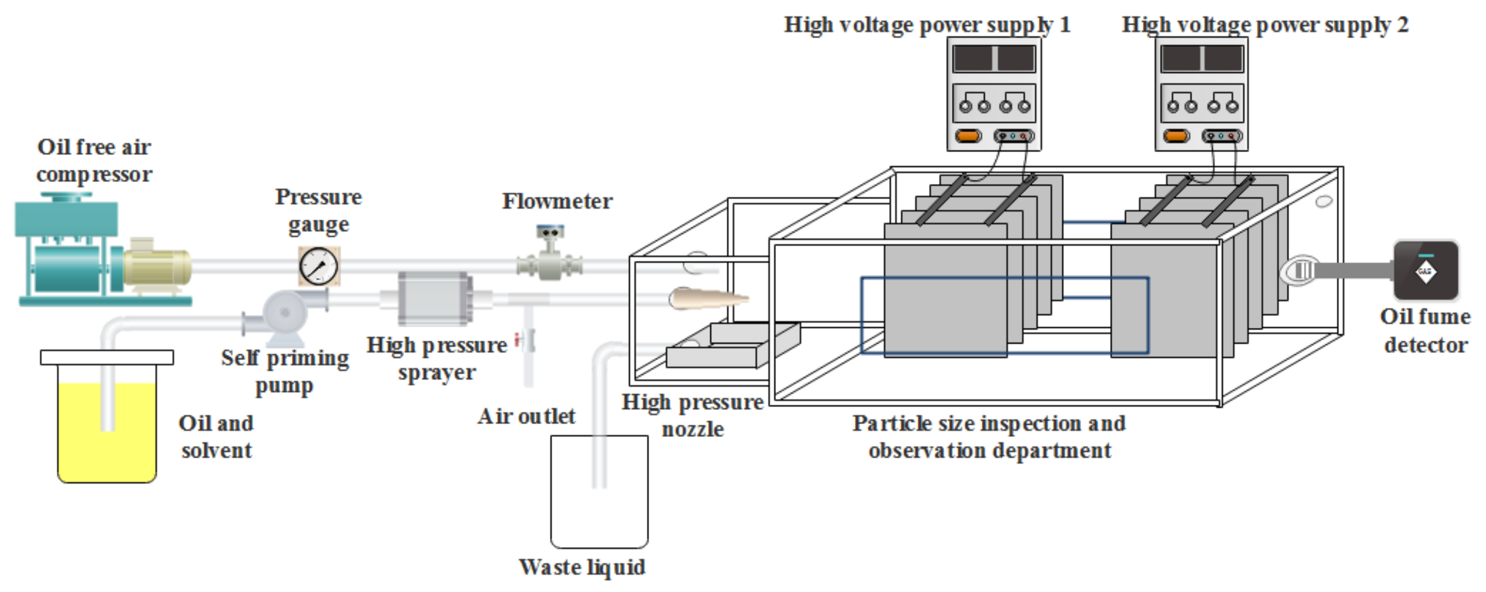
Figure 1 illustrates the experimental setup for catering oil droplet with electrostatic methods. The oil droplet was produced by high-pressure nozzle, and the droplet size could be adjusted by the nozzle pressure and the volume ratio of oil and organic solvent. The working pressure of the nozzle could be adjusted between 4–6 Mpa (40–60 kg). The 0–20 kV voltage was supplied by high voltage DC power supply (Pintech PA1030, Shenzhen, China). The concentration of the simulated cooking fume before and after treatment was measured by portable oil fume detector (TW-3068, Qingdao, China). The droplet size distribution was detected by spray particle size analyzer (Malvern Spraytec, Malvern, UK).

Figure 1.
Experimental setup for catering oil droplet purification.
2.2. Geometry Model
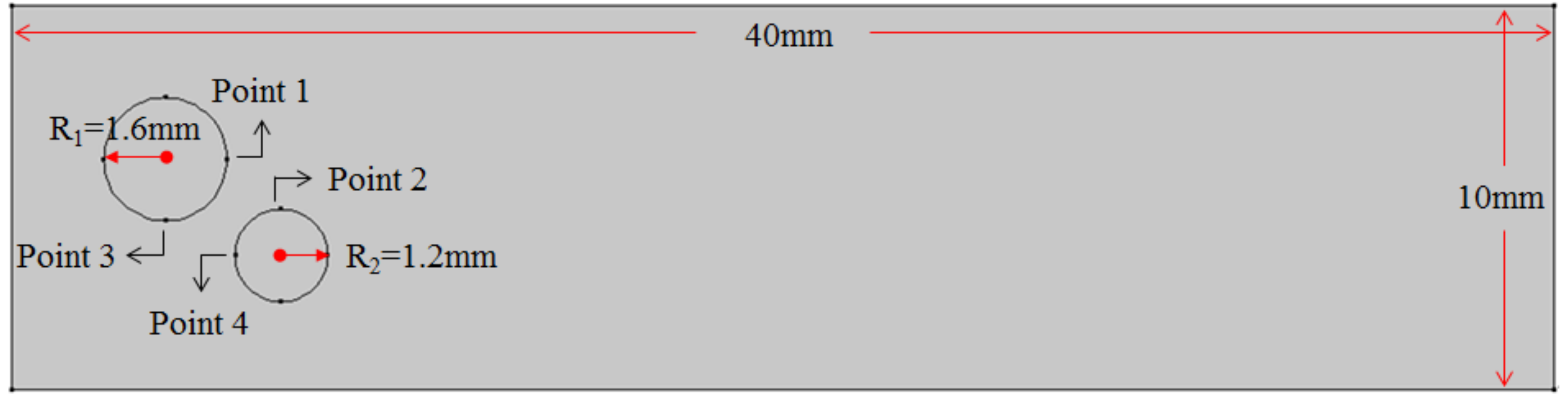
A two-dimensional finite element model was established by using COMSOL MultiphysicsTM to investigate the effects of voltage, flow speed and oil droplet radius on the change process of oil droplets. The model consisted of three parts, including a 40 mm × 10 mm rectangle, a large circle with a radius of 1.6 mm, whose center distance from the boundary was 4 mm and 6 mm, and a small circle with a radius of 1.2 mm, whose center with a distance of 7 mm and 3.5 mm, respectively. There were four measuring points on two circles, which were marked as points 1–4, respectively. The geometry of the model is shown in Figure 2.
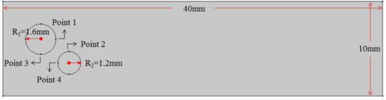
Figure 2.
Geometry model.
2.3. Numerical Methods
2.3.1. Boundary Condition
For simulation, electrostatic module, laminar flow module and phase field module were used for the project. The study on the effect of flow speed on oil droplets was carried out by the flow field module. The electrostatic module was used to study the effect of voltage on oil droplets. These two modules were especially used to study the change process of oil droplets. The integral module was filled with gas, which wrapped the oil droplets. Four measuring points were set on the oil droplets. The properties of components were set into the software. Once all values were set, the voltage, speed, pressure of the whole device were obtained.

Table 1.
The medium information setting in simulation process.
Table 2.
The setting parameter.
2.3.2. Mathematical Model
The coalescence of oil droplets is a complex and dynamic process. COMSOL was used to simulate the coalescence process, and a mathematical model was established based on flow field, electric field and phase field.
- (1)
- Governing equation of fluid motion
There are two substances in the model, oil and gas, which are immiscible with each other. The radius of oil droplet is very small. In electrokinesiology, it will be dominated by inertial force, viscous force, electric field force and so on, which will affect its motion state. For incompressible fluid, gravity is ignored. In the process of fluid motion, the fluid satisfies Navier–Stokes equation [31]
where u is the flow speed (m/s), ρ is the density (kg/m3), p is the pressure (Pa), I is the identity matrix, μ is the hydrodynamic viscosity (Pa∙s), Fst is the surface tension and FE is the electric field force.
The surface tension is the source term of Navier–Stokes equation, and its relationship with chemical potential G is
The expression of chemical potential G is
where η is the parameter characterizing interface thickness, λ is a parameter characterizing energy density.
In order to analyze the variation law of oil droplets under electric field, the phase field method based on Cahn–Hilliard equation [32,33,34] is used to control the deformation and coalescence process of oil droplets. The equation is as follows
where φ is phase holdup, γ is a constant, indicating the mobility of the interface.
In the phase field method, the Cahn–Hilliard equation is usually decomposed into the following form
The volume fractions Vf1 and Vf2 of the two phases can be obtained from the above equation
- (2)
- Electric field governing equation
According to Maxwell’s equation [35,36], in the flow of current body, due to the characteristic time of magnetic field, τm = ησl2 is shorter than that of electric field τe = ε/σ by a few orders of magnitude, so the magnetic field effect can be ignored.
When studying the dynamic behavior of oil droplets under the action of single electric field or coupled field, Maxwell’s equation is satisfied
where ε0 is the vacuum dielectric constant, taking 8.8542 × 10⁻¹² F/m, εr is the relative dielectric constant of the fluid, dimensionless, E is the electric field strength, U is the electric field potential (V).
The relationship between electric field intensity E and potential V is as follows
According to Equation (1), the electric field force is a source term of Navier–Stokes equation, which can be obtained through Maxwell stress tensor
The expression of Maxwell stress tensor T is
where I is the unit tensor.
2.3.3. Aggregation State Evaluation
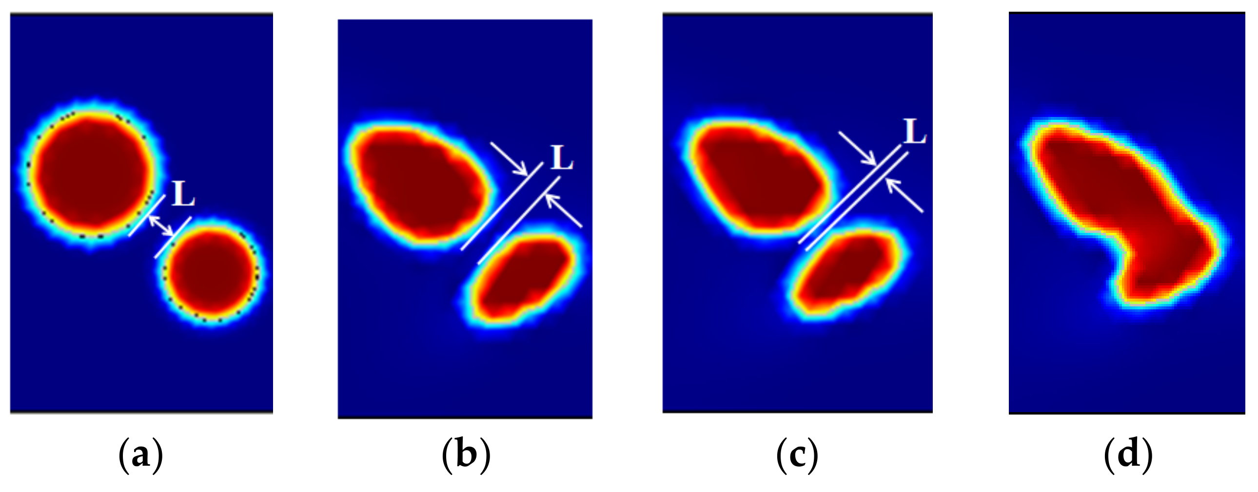
In this paper, the effect of oil droplets’ coalescence was evaluated by tsc of oil droplets, which was determined by the deformation degree (D) of oil droplets
where L is the shortest distance between any two tangents on the circles, Lo is the shortest distance in the initial state, Lt is the shortest distance at detected time. The judgment of oil drop deformation is shown in Figure 3.
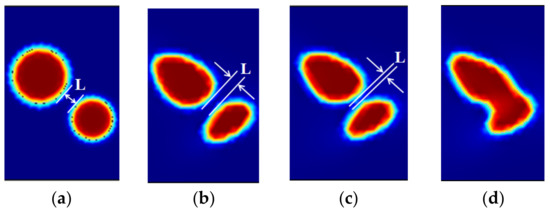
Figure 3.
Determination of oil droplet deformation. (a) Lt = 0.5 mm, (b) Lt = 0.3 mm, (c) Lt = 0.2 mm, (d) Lt = 0.
Figure 3a shows the original state, Lta = L0 = 0.5 mm, so Da = 0%, Ltb = 0.3 mm, Db = 40%, Ltc = 0.2 mm, Dc = 60%, accordingly. When Dd = 100%, the oil droplets began to coalesce, the corresponding time was defined as tsc. The larger the value of L was, the greater the degree of deformation of oil droplets was, the shorter tsc was and the better the coalescence state of oil droplets was.
2.3.4. Grid Independence Verification and Model Verification
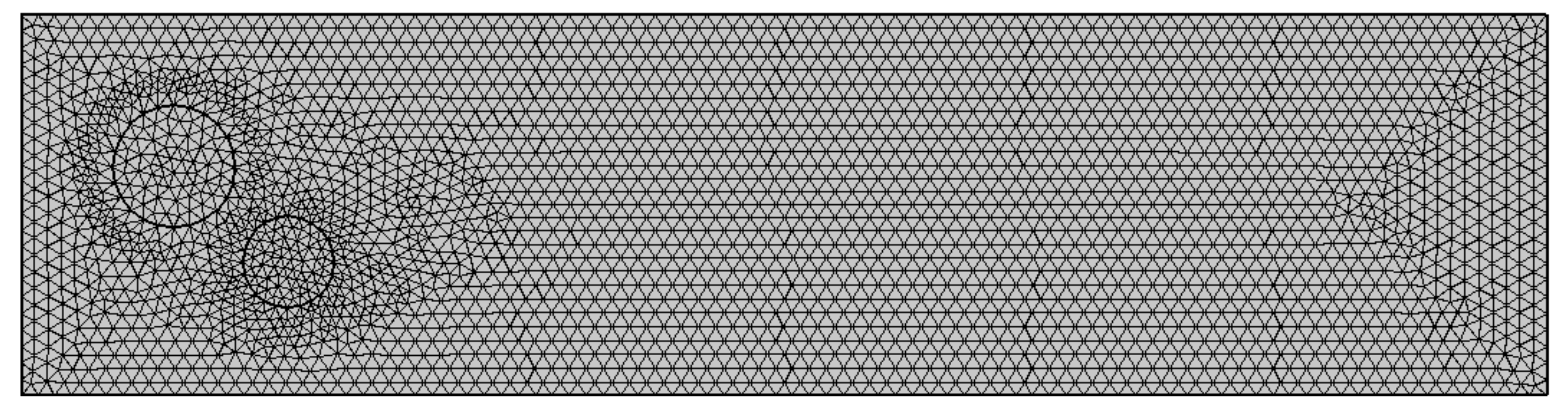
To reduce convergence problems and improve accurate calculations, the whole model was meshed by triangular grid. The simulation results of grids with different specifications are shown in the Figure 4a. The results indicated that the obtained results were not very dependent on either mesh size or mesh number in the tested situations. The coarsened triangular mesh (5848 elements) was chosen for further analysis because of its advantages of saving space and relatively fast processing.
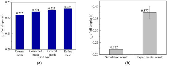
Figure 4.
Grid comparison results. (a) Simulation results; (b) comparison of simulation results and experimental results.
In Figure 4b, the comparison of experimental results by spray particle size analyzer (Malvern Spraytec, British) and the computed value by simulated method Is given. The meaning tsc was 0.377 s for three experiments, which was about 1.7 times of the corresponding simulated results with coarsened triangular mesh. The delay of tsc of experimental value might be caused by the test interval. On the whole, the two values in Figure 4 were in the same order of magnitude.
From these results, we found the results of numerical simulation were basically consistent with the experimental results, indicating that the simulation method was correct and reasonable. The geometric model division is shown in Figure 5.
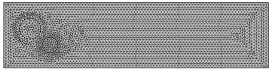
Figure 5.
Mesh-generation diagram.
3. Results and Discussion
3.1. Effect of Physical Field
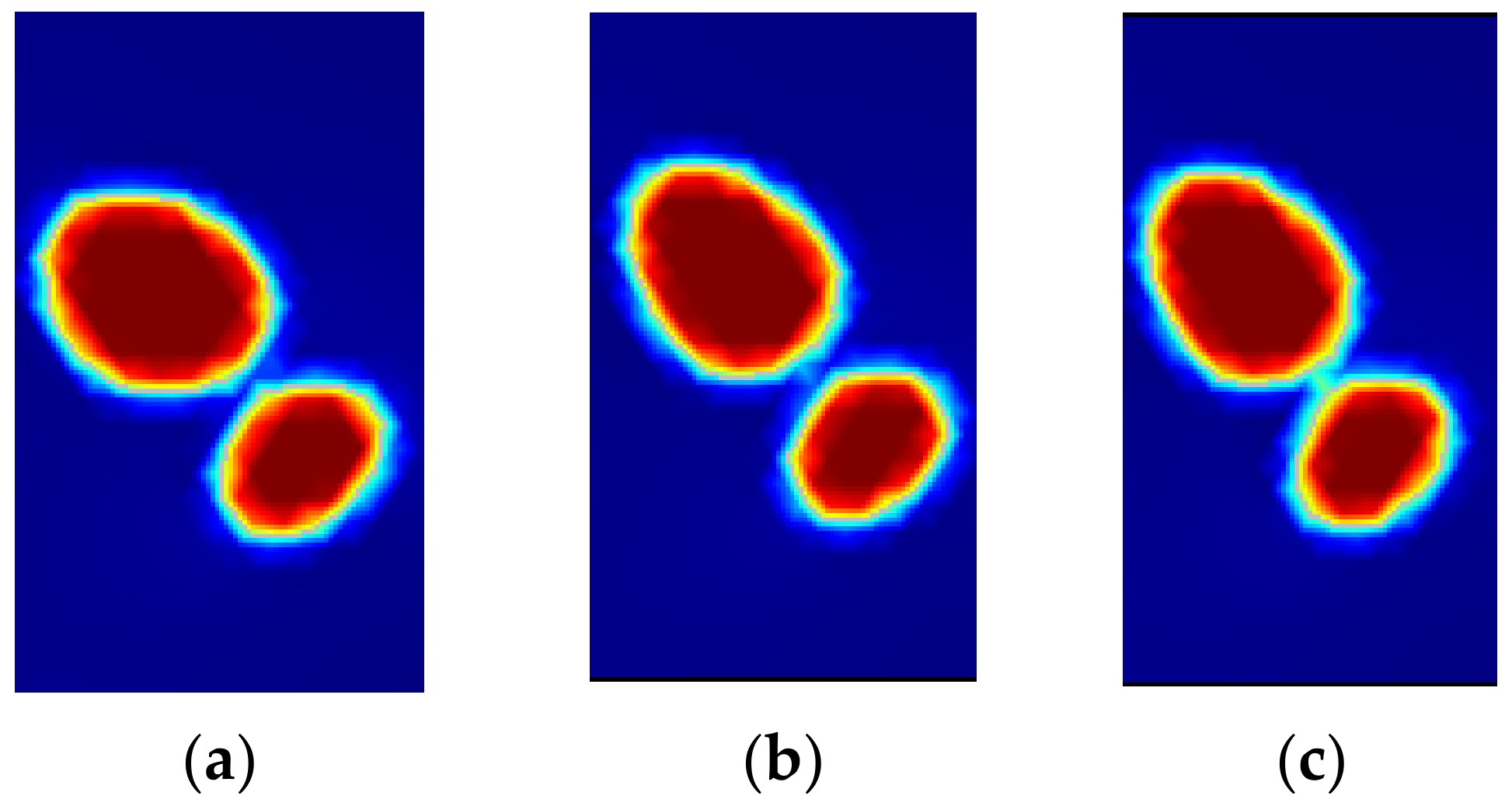
The actions of a single field and coupling field on oil droplets’ coalescence were compared, and voltage and flow speed were fixed as 10 kV and 0.05 m/s, respectively. The results are shown in Figure 6 when the recorded time was 0.2 s. The deformation degrees D of oil droplets were Da = 20%, Db = 40 mm and Dc = 68%, respectively. Compared with the single electric field and flow field, the coalescence speed in the coupled field was faster. The oil droplets deformed along the connection direction of the circle center, then elongated. The forces of the flow field and electric field on the oil droplets were layered, which promoted the coalescence of oil droplets. Therefore, the coupling field was selected for detailed analysis in this paper.
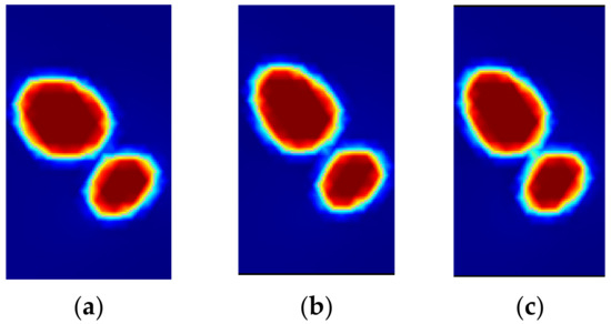
Figure 6.
Comparison of physical fields. (a) Flow field, (b) electric field, (c) coupling field.
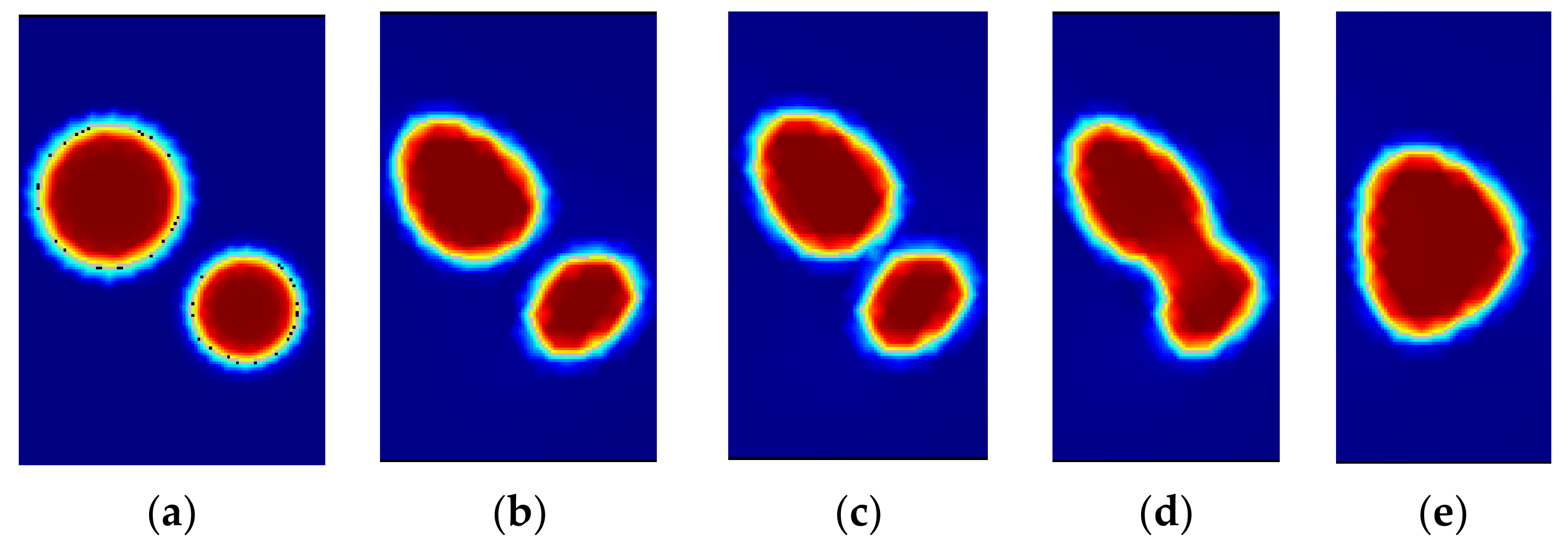
When voltage was 10 kV and the flow speed was 0.05 m/s, the process of oil droplets’ coalescence with time under the coupling field is shown in Figure 7.
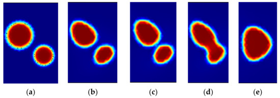
Figure 7.
Oil droplet coalescence process under the coupling of electric field and flow field. (a) 0 s, (b) 0.1 s, (c) 0.2 s, (d) 0.3 s, (e) 0.4 s.
The electrohydrodynamic flow related to oil droplets in the electric field would be impacted by the tangential electrical stress at the fluid interface [37]. The tangential viscous stress produced by the dynamic flow of the fluid was used to balance the tangential electric stress at the fluid interface. The surface of the oil droplets was pulled by local electric stress and viscous stress, which caused them to appear with various shapes, such as a flat sphere or a long ellipse. Oil droplets with a larger radius had a strong flow field effect, and dominated the coalescence process [38]. Small droplets moved along the flow direction of large droplets and were eventually integrated into large droplets to form a single droplet [39].
3.2. Influence of Various Factors on Coalescence Effect
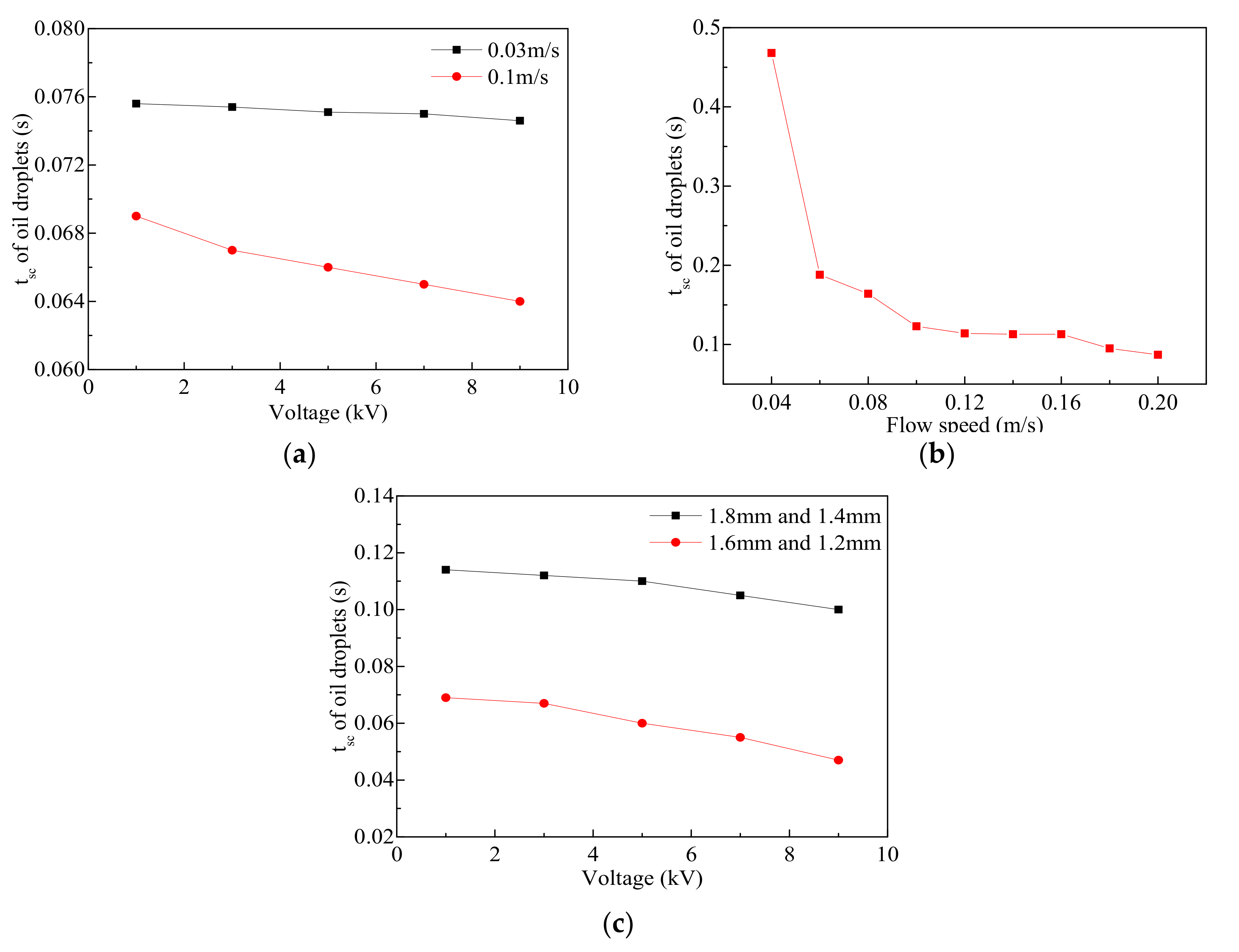
When the flow speed was 0.03 m/s and 0.1 m/s, tsc at different voltages (1–9 kV) are shown in Figure 8a. As stated in electrostatics theory [40], under the action of an electric field, the electric stress at the fluid interface pulls the oil droplets along the direction of the electric field, which might promote the coalescence of oil droplets. Thus, higher voltage meant the more obvious effect of the electric stress. When voltage was increased from 1 kV to 9 kV, the gathering speed was quickened, and tsc was shortened from 0.069 s to 0.064 s with 0.1 m/s flow speed. Meanwhile, the greater the flow speed was, the faster the oil droplets coalesced.
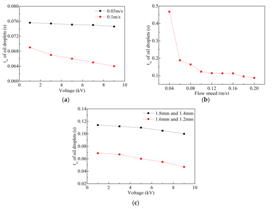
Figure 8.
Influence of various factors on coalescence effect. (a) Voltage, (b) flow speed, (c) radius.
As voltage was set as 10 kV, the influence of flow speed on tsc by computer simulation is shown in Figure 8b. When the flow speed was dropped from 0.04 m/s to 0.1 m/s, tsc decreased from 0.468 s to 0.123 s rapidly. Then the downward trend became gentle when the flow speed ranged from 0.1 m/s to 0.2 m/s. This notable difference might be attributed to the carrying effects on the oil droplets by the gaseous fluid with a higher flow speed, which would exacerbate the distortion of the oil droplets and speed up the oil droplets’ coalescence. When the flow speed was further increased to 0.5 m/s, the contact time between the oil droplets was too short and the interaction force between them was weakened, which made it difficult to promote oil droplets’ condensation.
In this paper, the effect of oil droplet radius on oil droplets’ coalescence was also simulated as shown in Figure 8c. Setting the flow speed as 0.5 m/s, and the radius of two oil droplets as 1.8 mm and 1.4 mm, 1.6 mm and 1.2 mm, respectively, the two oil droplets with the larger radius would acquire greater electric field force, which would promote them to being close together and make them easier to coalesce, which could then significantly enhance the coalescence speed.
The small oil droplet below in Figure 8c was merged in the wake flow area of the upper larger droplet. The larger the upper droplet size was, the greater the suction to the lower droplets was, which would promote the coalescence of the oil droplets. It could be inferred that properly increasing the oil droplet radius was conducive to the coalescence of the oil droplets.
In addition, the two oil droplets with the same diameter were placed in the simulated electric field to further investigate the impact of radius on coalescence process, as shown in Figure 9a. The oil radius was increased to a 0.05 mm interval, with 10 kV voltage and 0.5 m/s flow speed, and the correlation curve of the oil droplets’ coalescence time with oil droplet radius is shown in Figure 9b.
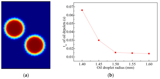
Figure 9.
Influence of oil droplet radius on coalescence effect of two same radius oil droplets. (a) Oil droplets with the same radius, (b) variation curve of tsc vs. oil droplet radius.
When the oil droplet size was enlarged from 1.4 mm to 1.5 mm, the amount of polarization charge generated by the electric field force on the surface of the oil droplets was raised, and the coalescence force between the oil droplets was accelerated, so tsc was knocked significantly. If the oil droplet radius was too large, the electric field force was dispersed, and the influence on the coalescence could be ignored. When the oil droplet radius was larger than 1.5 mm, the change in tsc was not obvious.
4. Simulation Optimization
4.1. Response Surface Analysis
In this paper, a series of tests were designed by Design Expert 8.0 software based on Box–Behnken response surface method. The factors and levels are listed in Table 3.
Table 3.
Response surface test factor level coding table.
Based on the simulation results, the quadratic multinomial regression equation related to tsc and the influencing factors was obtained as follows
According to the interaction synergy coefficient in formula 14, AC and BC were synergistic. There was antagonism between A and B. When the oil droplet radius was 1.56 mm, the voltage was 12 kV and the speed was 180 mm/ms; the shortest tsc was 16.8253 ms.
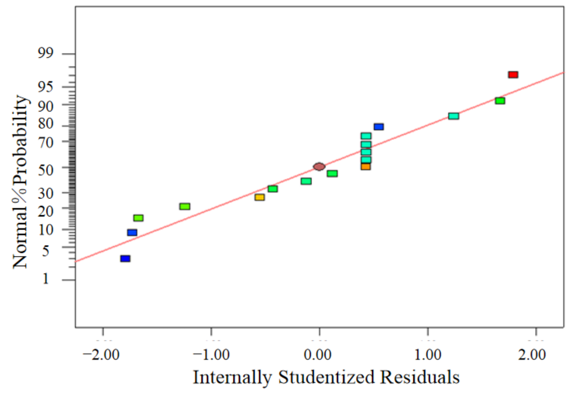
On the whole, the experimental values are distributed around the predicted values in Figure 10, which indicates that the actual values were similar to the predicted values. The accuracy of model fitting was verified.
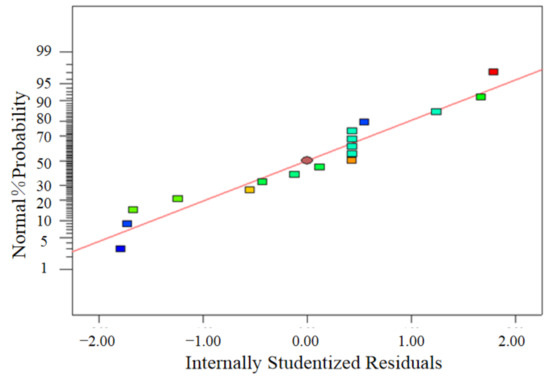
Figure 10.
Comparison between predicted and actual values of different factors.
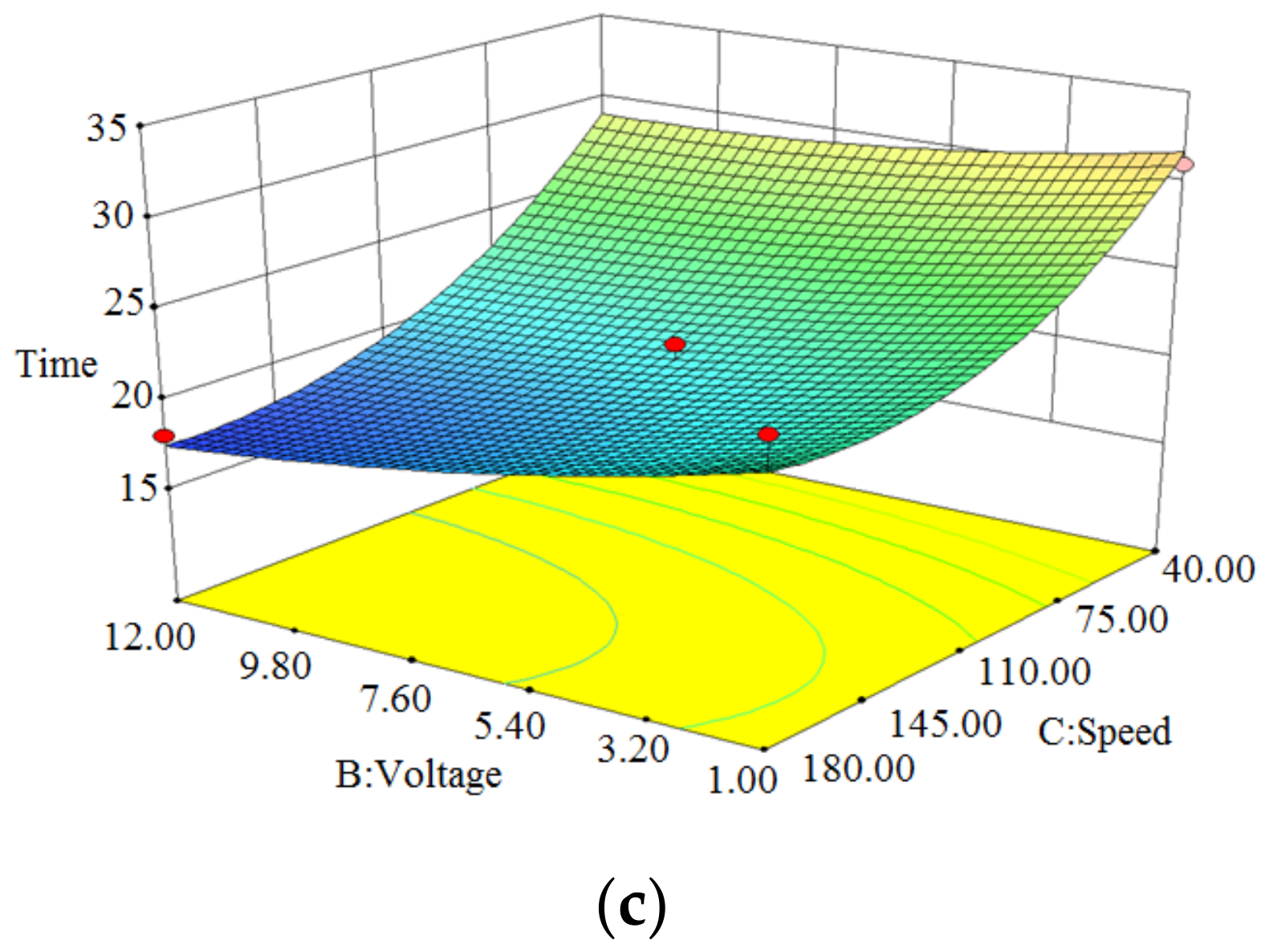
The 3D response surface diagram of the model (Figure 11) was obtained using the software, which not only showed the influence of a single factor, but also reflected the strength of the interaction of various factors. When the bending degree of the curve and the inclination of the surface were large, it indicated that this group of interactions had an obvious impact on the results.
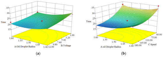

Figure 11.
Response surface diagram of interaction of various factors. (a) Radius and voltage, (b) radius and speed, (c) voltage and speed.
Figure 11a shows the effect of the interaction of the radius and voltage on tsc at a speed of 110 mm/ms. When the voltage was set as a constant, tsc increased slightly with the decrease in radius. When the radius of an oil droplet was fixed, the voltage decreased and tsc increased. The curves on the bottom surface were flatter and showed a slight upward trend as the influence factor increased. The increase in voltage made the oil droplets subject to greater electrical stress. However, with the increase in radius, the volume of the oil droplets became larger and the force was dispersed. Therefore, the coalescence of the oil droplets was less affected by the interaction between them.
Figure 11b shows the effect of the interaction of the radius and speed on tsc at a voltage of 6.5 kv. The interaction of these two factors had a significant influence on the effect of oil droplets’ coalescence. The increase in speed produced a larger carrying force, while the increase in oil droplet radius caused the oil droplets to be affected by a larger electric field. The two forces acted on the oil droplets together to accelerate the coalescence of oil droplets.
Figure 11c shows the effect of the interaction of voltage and speed on tsc when the oil droplet radius was 1.5 mm. When the voltage increased, tsc decreased because the oil droplets were subjected to increased electric stress. As the speed decreased, tsc increased. The carrying effect of speed and the electrical stress of voltage overlapped each other, which promoted the coalescence of oil droplets. The interaction effect of the two factors on the coalescence of oil droplets was similar to that of radius and speed.
In summary, the effect of the interaction of voltage and speed on tsc was similar to that of radius and speed. The interaction of oil droplet radius and voltage had a weak effect on the coalescence of oil droplets. The influence degree of each factor was speed > voltage > radius of oil droplet.
4.2. Matrix Correlation Analysis
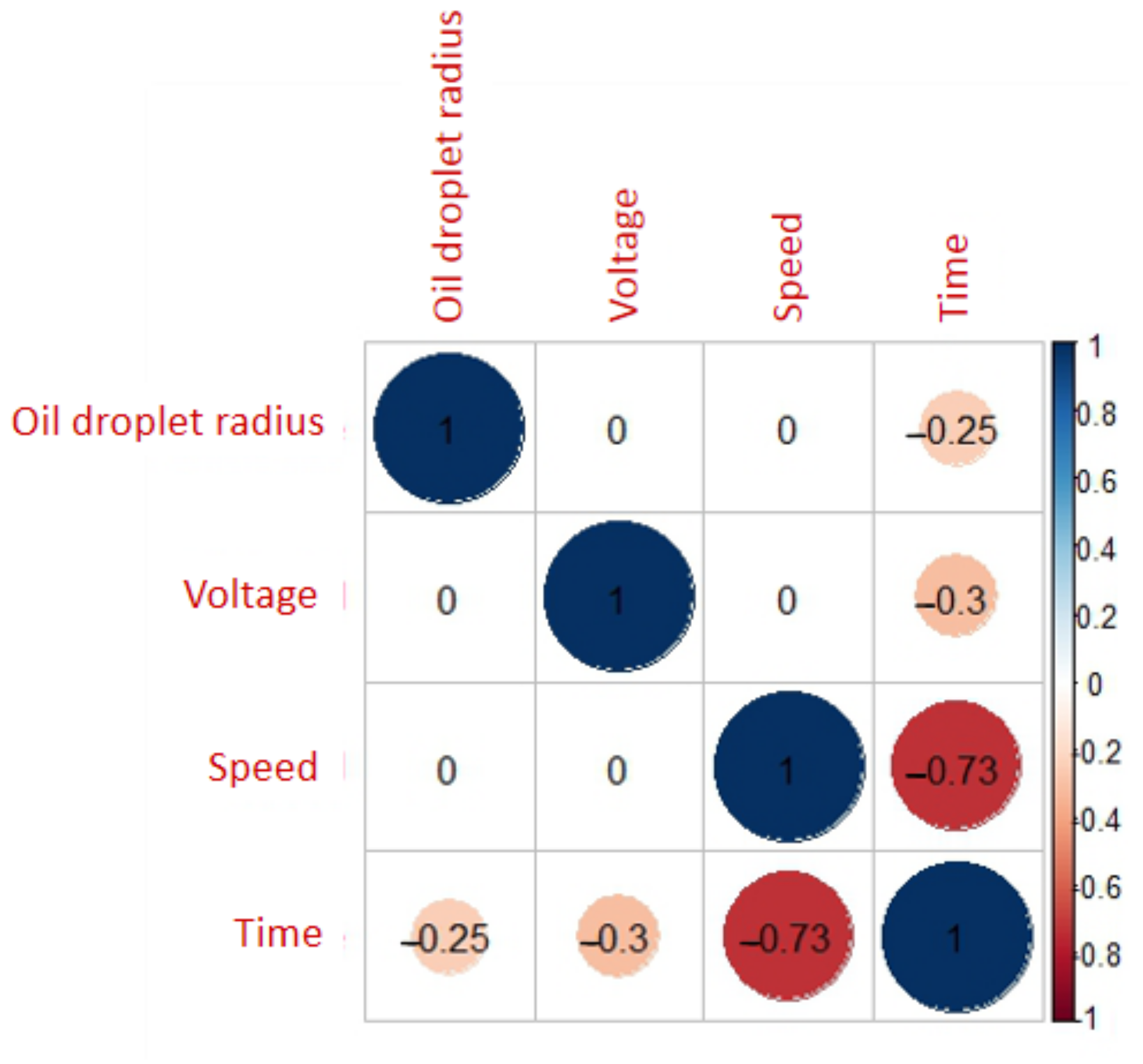
In addition to the response surface method, the Pearson correlation coefficient was an effective method to study the linear correlation between two data sets. The resultant correlation matrix was visualized in a heatmap format, which was generated using the “corrplot” package via R software.
The correlation between tsc and the three main parameters affecting oil droplet coalescence speed was assessed using this method. The larger the absolute value was, the greater the influence of various factors on time was. “−” indicates that the two factors were negatively correlated, and “+” indicates that the two factors were positively correlated.
As can be seen from Figure 12, there was no linear relationship among oil droplet radius, voltage and speed. The influence degree of each factor was in the order of speed > voltage >oil droplet radius, and all of them were negatively correlated with time. tsc was shortened with the increase in speed, voltage and oil droplet radius. Increasing the speed enhanced the effect of the flow field on oil droplets, which increased the carrying capacity of the entire oil droplet. The polarized charge was dispersed on the surface of the droplet, and its influence on the droplet was dispersed. The effect of electric stress on the droplet was also weaker than that of the flow field. Therefore, the speed had the greatest influence on the coalescence of oil droplets.

Figure 12.
Matrix correlation analysis.
Through the analysis of Matrix correlation and response surface, the conclusion was completely consistent with the test results. Based on this result, in practice, the coalescence effect of oil droplets can be effectively improved by adjusting the parameters of flow speed.
5. Conclusions
In the paper, COMSOL software was used to simulate and analyze the electrostatic coalescence of oil droplets under the coupling field of the electric field and flow field. The parameters were optimized by response surface and Matrix correlation, and the following conclusions were drawn as follows:
- 1.
- The shortest distance between any two tangents on the circles (L), the time of starting coalescence (tsc) and the degree of deformation (D) were used to determine the coalescence effect; compared with experimental results, the module was feasible.
- 2.
- The coupling field of the electric field and flow field was better than that of the single field.
- 3.
- The increase in voltage, flow speed and oil droplet radius promoted the coalescence of oil droplets. There was an optimal range of flow speed and oil droplet radius. When the flow speed exceeded 0.5 m/s, oil droplets were difficult to coalesce. When the radius of oil droplets was in the range of 0–1.5 mm, it was more conducive to the coalescence of oil droplets.
- 4.
- The simulation results were analyzed in detail by the response surface method and Matrix correlation method. The influence degree of each factor was speed > voltage > oil droplet radius. The research results obtained can be applied to device design and process parameter optimization.
Author Contributions
Conceptualization: D.X. and L.Z.; Data curation: D.X.; Formal analysis: D.X. and J.G.; Investigation: J.G.; Validation: Z.Y.; Visualization: M.J. All authors contributed equally to the analysis and in writing the paper. All authors have read and agreed to the published version of the manuscript.
Funding
This study is funded by the Beijing Great Wall scholar training program (CIT& TCD20190314) and the important scientific research achievement training program of Beijing Institute of Petrochemical Technology (BIPTACF-003). University student scientific research and training program (2022J00138).
Institutional Review Board Statement
Not applicable.
Informed Consent Statement
Not applicable.
Data Availability Statement
All data used in this study are available upon request.
Acknowledgments
This study is funded by the Beijing Great Wall scholar training program (CIT& TCD20190314) and the important scientific research achievement training program of Beijing Institute of Petrochemical Technology (BIPTACF-003). University student scientific research and training program (2022J00138). We appreciate them.
Conflicts of Interest
The authors declare no conflict of interest.
References
- Zhang, X.; Qian, Z.; Zhang, D.; Zhu, T.; Yuan, Q.; Ye, Z. Research progress of cooking fume emission characteristics and purification technologies. Environ. Eng. 2020, 38, 37–41. [Google Scholar]
- Contal, P.; Simao, J.; Thomas, D.; Frising, T.; Callé, S.; Appert-Collin, J.C.; Bémer, D. Clogging of fibre filters by submicron droplets. Phenomena and influence of operating conditions. J. Aerosol Sci. 2004, 35, 263–278. [Google Scholar] [CrossRef]
- Mullins, B.J.; Mead-Hunter, R.; Pitta, R.N.; Kasper, G.; Heikamp, W. Comparative performance of philic and phobic oil-mist filters. AIChE J. 2014, 60, 2976–2984. [Google Scholar] [CrossRef]
- Li, R.; Xu, A.; Zhao, Y.; Chang, H.; Li, X.; Lin, G. Genetic algorithm (GA)—Artificial neural network (ANN) modeling for the emission rates of toxic volatile organic compounds (VOCs) emitted from landfill working surface. J. Environ. Manag. 2022, 305, 114433. [Google Scholar] [CrossRef] [PubMed]
- Tan, J.; Li, W.; Ma, C.; Wu, Q.; Xu, Z.; Liu, S. Synthesis of Honeycomb-Like Carbon Foam from Larch Sawdust as Efficient Absorbents for Oil Spills Cleanup and Recovery. Materials 2018, 11, 1106. [Google Scholar] [CrossRef] [PubMed] [Green Version]
- Zhang, S.; Liu, S.; Chen, Q. Particle capture by a rotating disk in a kitchen exhaust hood. Aerosol Sci. Technol. 2020, 54, 929–940. [Google Scholar] [CrossRef]
- Gao, W.; Cao, D.; Lv, K.; Wu, J.; Wang, Y.; Wang, C.; Wang, Y.; Jiang, G. Elimination of short-chain chlorinated paraffins in diet after Chinese traditional cooking-a cooking case study. Environ. Int. 2019, 122, 340–345. [Google Scholar] [CrossRef]
- Li, C.; Bai, L.; He, Z.; Liu, X.; Xu, X. The effect of air purifiers on the reduction in indoor PM2.5 concentrations and population health improvement. Sustain. Cities Soc. 2021, 75, 103298. [Google Scholar] [CrossRef]
- Wang, P.; Jiang, J.; Li, S.; Yang, X.; Luo, X.; Wang, Y.; Thakur, A.K.; Zhao, W. Numerical investigation on the fluid droplet separation performance of corrugated plate gas-liquid separators. Sep. Purif. Technol. 2020, 248, 117027. [Google Scholar] [CrossRef]
- Gao, L.; Lu, Y. Present status and improvement of indoor air purifier. J. Harbin Inst. Technol. 2004, 36, 199–201. [Google Scholar]
- Kiev, I. Electrostatic Precipitator. U.S. Patent 20200188932A1, 29 December 2020. [Google Scholar]
- Sarkola, J. An Electrostatic Filter and a Rack for Filter Plates of an Electrostatic Filter. U.S. Patent 20200246808A1, 22 February 2018. [Google Scholar]
- Wang, J.; Wang, X.; Dong, D. Research on Air Pollution Problems and Corresponding Countermeasures in China’s Catering Industry. Environ. Sci. Technol. 2019, 32, 6. [Google Scholar]
- Li, Y.; Li, J.; Li, H. Cooking fume Pollution and Its Purification Technology. Sichuan Chem. Ind. 2018, 21, 13–16. [Google Scholar]
- Qi, L.; Yuan, Y. Characteristics and the behavior in electrostatic precipitators of high-alumina coal fly ash from the Jungar power plant, Inner Mongolia, China. J. Hazard. Mater. 2011, 192, 222–225. [Google Scholar] [CrossRef] [PubMed]
- Ruttanachot, C.; Tirawanichakul, Y.; Tekasakul, P. Application of Electrostatic Precipitator in Collection of Smoke Aerosol Particles from Wood Combustion. Aerosol Air Qualres. 2011, 11, 90–98. [Google Scholar] [CrossRef]
- Adamiak, K. Numerical models in simulating wire-plate electrostatic precipitators: A review. J. Electrost. 2013, 71, 673–680. [Google Scholar] [CrossRef]
- Ni, M.; Yang, G.; Wang, S.; Wang, X.; Xiao, G.; Zheng, G.; Gao, X.; Luo, Z.; Cen, K. Experimental investigation on the characteristics of ash layers in a high-temperature wire-cylinder electrostatic precipitator. Sep. Purif. Technol. 2016, 159, 135–146. [Google Scholar] [CrossRef]
- Zhu, J.; Zhang, X.; Chen, W.; Shi, W.; Yan, K. Electrostatic precipitation of fine particles with a bipolar pre-charger. J. Electrost. 2010, 68, 174–178. [Google Scholar] [CrossRef]
- Zhang, X.; Bo, T.L. The effectiveness of electrostatic haze removal scheme and the optimization of electrostatic precipitator based on the charged properties of airborne haze particles: Experiment and simulation. J. Clean. Prod. 2020, 288, 125096. [Google Scholar] [CrossRef]
- Feng, Z.; Cao, S.; Wang, J.; Kumar, P.; Haghighat, F. Indoor airborne disinfection with electrostatic disinfector (ESD): Numerical simulations of ESD performance and reduction of computing time. Build. Environ. 2021, 200, 107956. [Google Scholar] [CrossRef]
- Fan, X. Research on the High Voltage Electrostic Precipitation with DC-AC Alternating Technology; Beijing Jiaotong University: Beijing, China, 2014. [Google Scholar]
- Jaworek, A.; Marchewicz, A.; Krupa, A.; Sobczyk, A.T.; Czech, T.; Antes, T.; Śliwiński, L.; Kurz, M.; Szudyga, M.; Rożnowski, W. Dust particles precipitation in AC/DC electrostatic precipitator. J. Phys. Conf. Ser. 2015, 646, 12031. [Google Scholar] [CrossRef]
- Jaworek, A.; Marchewicz, A.; Sobczyk, A.T.; Krupa, A.; Czech, T. Two-stage electrostatic precipitator with dual-corona particle precharger for PM2.5 particles removal. J. Clean. Prod. 2017, 164, 1645–1664. [Google Scholar] [CrossRef]
- Xiong, H. Design and Research on Efficient Electrostatic Coalescer for Crude Oil Dehydration; Beijing Institute of Petrochemical Technology: Beijing, China, 2016. [Google Scholar]
- Chang, Y. Research on the Droplet Movement in Electrowetting on Dielectric Based Ditigal Microfluidic System; Hebei University of Technology: Tianjing, China, 2018. [Google Scholar]
- Yin, Y. Numerical Simulation and Experimental Study of High Efficiency Electrostatic Coalescence Separation for Crude Oil Dehydration; Hebei University of Technology: Tianjing, China, 2018. [Google Scholar]
- Zhu, Z. Numerical Simulation and Study on Mechanism of Droplet Coalescence under Electrostatic Fields; Jiangsu University: Zhenjiang, China, 2017. [Google Scholar]
- Yu, S.; Jian, L.; Chong, Z. A local and parallel Uzawa finite element method for the generalized Navier–Stokes equations. Appl. Math. Comput. 2019, 8, 124671. [Google Scholar]
- DB11/1488-2018; Emission Standards of Air Pollutants for Catering Industry. Ministry of Ecology and Environment of the People’s Republic of China: Beijing, China, 2018.
- Chakraborty, A.; Warrior, H.V. Study of turbulent flow past a square cylinder using partially-averaged Navier-Stokes method in Open FOAM. Arch. Proc. Inst. Mech. Eng. Part C J. Mech. Eng. Sci. 2020, 234, 2821–2832. [Google Scholar] [CrossRef]
- Schreyer, L.; Hilliard, Z. Derivation of generalized Cahn-Hilliard equation for two-phase flow in porous media using hybrid mixture theory. Adv. Water Resour. 2021, 149, 103839. [Google Scholar] [CrossRef]
- Ren, H.; Zhuang, X.; Trung, N.T.; Rabczuk, T. Nonlocal operator method for the Cahn-Hilliard phase field model. Commun. Nonlinear Sci. Numer. Simul. 2020, 96, 105687. [Google Scholar] [CrossRef]
- Fu, G. A divergence-free HDG scheme for the Cahn-Hilliard phase-field model for two-phase incompressible flow. J. Comput. Phys. 2020, 419, 109671. [Google Scholar] [CrossRef]
- Stefański, T.; Gulgowski, J. Fundamental properties of solutions to fractional-order Maxwell's equations. J. Electromagn. Waves Appl. 2020, 34, 1955–1976. [Google Scholar] [CrossRef]
- He, B.; Yang, W.; Wang, H. Convergence analysis of adaptive edge finite element method for variable coefficient time-harmonic Maxwell’s equations. J. Comput. Appl. Math. 2020, 376, 112860. [Google Scholar] [CrossRef]
- Cheng, M.; Hua, J.; Lou, J. Simulation of bubble–bubble interaction using a lattice Boltzmann method. Comput. Fluids 2010, 39, 260–270. [Google Scholar] [CrossRef]
- Wang, X. Experimental and Simulation Study on Oil Droplet Upward Movement in Water; Hebei University of Technology: Tianjing, China, 2017. [Google Scholar]
- Feng, J. Electrohydrodynamic behaviour of a drop subjected to a steady uniform electric field at finite electric Reynolds number. Proc. R. Soc. A Math. Phys. Eng. Sci. 1999, 455, 2245–2269. [Google Scholar] [CrossRef]
- Basaran, O.A.; Scriven, L.E. Axisymmetric shapes and stability of charged drops in an external electric field. Phys. Fluids A Fluid Dyn. 1989, 1, 799–809. [Google Scholar] [CrossRef]


Publisher’s Note: MDPI stays neutral with regard to jurisdictional claims in published maps and institutional affiliations. |
© 2022 by the authors. Licensee MDPI, Basel, Switzerland. This article is an open access article distributed under the terms and conditions of the Creative Commons Attribution (CC BY) license (https://creativecommons.org/licenses/by/4.0/).