Abstract
As a large-scale ocean–atmosphere coupling system in the Southern Hemisphere, the Antarctic Circumpolar Wave (ACW) greatly impacts the global climate. However, the interdecadal variation of the ACW has rarely been studied due to the lack of long-term data. In this research, the latest 20th Century Reanalysis Version 3 dataset is used to analyze the interdecadal variations of sea level pressure (SLP) and sea surface temperature (SST) signals in the ACW during 1836–2015. The results indicate that the ACW has not always been present in the recent 180 years, and it has remarkable interdecadal variations. Specifically, the ACW was hard to distinguish before the 1870s. The SLP anomalies propagated eastwards over the South Pacific and South Atlantic during part of the 1880s–1940s. The SST anomalies also have an eastward propagation in the 1880s–1960s. The most active period of the SLP signal is in the 1950s–1990s, while that of the SST signal is in the 1980s–1990s. The ACW has not been significant since the 21st century. The interdecadal variation of the SLP may be related to the variations of the long-term Southern Annular Mode and Pacific-South American pattern, while the interdecadal variation of the SST is more associated with the ENSO.
1. Introduction
By analyzing the monthly anomalies of the sea surface temperature (SST), meridional wind stress, sea level pressure (SLP) and sea ice extent in the Southern Ocean from the 1980s to the mid-1990s, White and Peterson, in 1996 (hereafter WP96), found that these variables have eastward-propagating signals around the pole, i.e., Antarctic Circumpolar Wave (ACW) [1]. This is the first time that the ACW has been proposed. The oscillation period of the ACW is 4–5 years, and it circles the Antarctic once in 8–10 years on average, showing a zonal wavenumber-2 (ACW-2) pattern in the Southern Ocean. This large-scale interannual oceanic and atmospheric phenomenon has attracted great attention from researchers, and it was soon confirmed by several other studies on various variables, such as surface air temperature, sea surface height and salinity, becoming the front topic in climate research [2,3,4]. Subsequently, an east-propagating zonal wavenumber-3 (ACW-3) pattern, which has approximately the same period as the ACW-2, has been identified in model simulations [5,6]. Although the ACW formation and maintenance mechanisms are still unclear, it is well established that the ACW consists of the ACW-2 and ACW-3. Cai and Baines in 2001 (hereafter CB01) and others proposed that the ACW-2 signal is highly correlated with the tropical El Niño Southern Oscillation (ENSO) activities mediated by the Pacific-South American (PSA) pattern and Southern Annular Mode (SAM) [7,8,9]. The ACW-3 signal is an eastward-propagating wavenumber-3 structure over the Southern Ocean, mainly caused by local air–sea interaction. It used to be considered a controversial quasi-standing pattern [9,10], but recent work has shown this issue probably comes from the mixture with others [11]. As an essential component of the climate in the Southern Hemisphere (SH) on the interdecadal time scale, the ACW greatly affects the Southern Ocean and SH climate change [12]. For example, White and Annis (hereafter WA04) suggested that the interdecadal variation of ENSO in the last half of the 20th century can be largely explained by the ACW variation [13]. Moreover, the ACW is a crucial indicator for characterizing the annual temperature and seasonal precipitation in New Zealand and parts of Australia [14,15]. A dipole-like oscillation was identified in the Southern Pacific, which connected the ACW with South American precipitation [16]. Besides SH, the ACW can expand its influence in the Northern Hemisphere through cross-equatorial airflows, such as the influence on the Indian summer monsoon rainfall and the East China summer rainfall [17,18]. Therefore, identifying the presence and decadal variation of the ACW over a long historical period can improve the understanding of the response to climate change in the SH and favor regional climate prediction.
In previous studies, the ACW from the 1980s to 1990s was confirmed to be highly active based on various observations [19,20,21]. However, few researchers have discussed the interdecadal variation of the ACW over a longer time scale, objectively due to the lack of long-term observations covering middle and high latitudes of the SH before satellites were widely used for meteorological observations. The satellite observations after 1979 are too short in duration for interdecadal research, while long-term station records may be long enough but hardly represent the propagating property of the ACW over the whole Sub-Antarctic Zone. One way to avoid this problem is to perform ACW numerical simulations [3,5,11]. However, due to the performance differences and simulation capability deficiencies of different numerical models, the ACW simulated in these studies differs in wavelength, periodical variation, amplitude, and other characteristics. Among them, some ACW simulations differ significantly from the actual observed ACW signals and have caused several disputes [22,23]. Proxy data, which was reconstructed based on records, such as ice core, are another solution. Unfortunately, these data often suffer from low temporal resolution and poor representativeness [24]. With the development of data assimilation and reanalysis techniques, long-term reanalysis data fused with observations and numerical simulations have recently been more widely applied to ACW research, and numerous achievements have been achieved in terms of the interdecadal variation [9,25,26]. Since different studies used different reanalysis datasets and extraction methods, the ACW signals slightly differ in these researches. Although the ACW does not exist stably in the past several decades, the interdecadal variation in its activity is commonly recognized.
Recently, the National Oceanic and Atmospheric Administration (NOAA), Cooperative Institute for Research in Environmental Sciences (CIRES) and the U.S. Department of Energy (DOE) have released the latest version of the NOAA–CIRES–DOE 20th Century Reanalysis (20CRV3) dataset with improved quality in the SH, whose starting time has been updated to the early nineteenth century. Inspired by the long-term dataset, we aim to identify the ACW in the last 180 years and analyze its interdecadal variation in this study. Following many previous works, we focus on SLP and SST, which come from the atmosphere and ocean, respectively. In addition, several large-scale climate signals associated with the ACW are investigated to explain its interdecadal variation. For previous studies, the ACW was typically investigated in a single variable or separated variable fields [24,27] ([28] hereafter GM13), and these researches ignored the strongly coordinated variations of different variables in the ocean–atmosphere coupling system [1,8,10]. Hence, we use the singular value decomposition (SVD) to reveal the corresponding ocean–atmosphere interactions.
The rest of this paper is organized as follows. Section 2 briefly introduces the data and analysis methods used in this study. Section 3 discusses the interdecadal variations of several climate indices investigated in this research. Section 4 presents the analysis results, where the results of the SLP, SST and SVD are shown in Section 4.1, Section 4.2 and Section 4.3, respectively. Finally, the conclusions and discussion can be obtained in Section 5.
2. Data and Methods
2.1. Data
The monthly mean SLP, SST, and 850 hPa and 500 hPa geopotential heights used in this research are derived from the 20CRV3 dataset from 1836 to 2015, with a spatial resolution of 1° × 1°. For this new version of the 20th Century Reanalysis Project, an improved 80-member ensemble Kalman filter, including an adaptive inflation algorithm is used to assimilate a larger set of surface pressure observations (from ISPD version 4.7) into an updated NCEP Global Forecast System (GFS) model, version 14.0.1. With this, in addition, a spectral horizontal resolution of T254 (nearly 0.5 degrees) and a vertical atmospheric resolution of 64 levels up to about 0.3 hPa are used, thus improving the confidence of this dataset in the SH [29]. Several issues should be noted, especially compared with other datasets, such as the sea ice concentrations and different grid resolutions. Additional attention should be paid to the radiative forcing prior to 1850. These issues are briefly introduced in ‘Model Notes’ on the download website. To diminish the unreliable records in Antarctica and exclude the strong variations of climate signals in the tropics, we focused on the middle to high latitudes where the ACW appears, and the research domain was restricted to the zone of 40° S–70° S as GM13 [28], while the ACW area was 56° S–66° S. The long-term SLP observation records from the stations Orcadas (60°44′ S, 44°45′ W) and Faraday (65°15′ S, 64°16′ W) were used for comparative analysis [30]. The correlation coefficients between the interpolated 20CRV3 data and observations are 0.85 (from 1904 to 1955, p < 0.01) for station Orcadas and 0.96 (from 1951 to 2015, p < 0.01) for station Faraday. Hence, the 20CRV3 reanalysis data can be considered reliable for use in this study.
2.2. Analysis Methods
Following the method from the WP96, the monthly climatologies over 180 years are subtracted from monthly SLP and SST values to remove the seasonal cycle and obtain the monthly anomalies. Since the oscillation period of the ACW is 4–5 years, the 6-order Butterworth filter with a passing window of 3–7 years was applied to the monthly anomaly signals to highlight the interannual variations of climate elements, which remain as the ACW. Note that the data from three years before and after the study period were omitted because of the boundary effect of the filter. To separate the ACW-2 and ACW-3 signals and discuss their variations and influence on large-scale climate change, we used the Empirical Orthogonal Function (EOF) method to extract the leading modes, as in the CB01 and GM13 [8,28]. Prior to the EOF analysis, the grid data should be multiplied by the square root of the cosine of latitudes to perform the area weighting. Then, the ACW is reconstructed by the main corresponding EOF modes. Moreover, the meridional average provides a time-longitude diagram to display the ACW interdecadal variation visually. Compared with the EOF, which extracts the principal mode of one field, the SVD can find the coupled mode pairs in two fields [31]. In this research, we normalized the filtered SLP and SST to the same order of magnitude, and then they were used as the left and right fields for the SVD analysis. The SVD significance test was carried out using the Monte Carlo method.
3. Large-Scale Climate Indices
In order to characterize the large-scale patterns that significantly impact the ACW, we introduced multiple climate indices in this study. The SAM is the dominant pattern of the SH atmospheric circulations, identified by the SAM index defined by Thompson and Wallace ([32] hereafter TW00). That is, the SAM index can be obtained based on the leading principal component (PC) of 850 hPa monthly anomalies in the south of 20° S. For convince of comparison, we chose the (arbitrary) sign of the leading EOF and its PC in the same way as TW00. This definition can theoretically capture the comprehensive feature of the pressure difference at the middle and high latitudes in the SH, which is more representative of the SH atmospheric circulation than the other prevalent method proposed by Gong and Wang [33] and more applicable to the ACW study. The results from this research show that the leading EOF pattern at 850 hPa is characterized by the seesaw of two concentric circles between the high latitudes and parts of the mid-latitudes, which contributes 29.5% of the variability, consistent with the conclusion of the TW00 (Figure 1a). Further, the other SAM index series from the 20CRv2c dataset was also used for comparison, which was defined by Gong and Wang [33]. The correlation coefficient between the two SAM series is 0.82 (p < 0.01) during 1851–2011, proving that the SAM index adopted in this study can capture the SAM variation. Since the SAM are represented on different time scales, a low-pass Lanczos filter was performed to retain low-frequency SAM signals beyond the 2-year period. To further reveal the low-frequency variation, we calculated the cumulative values of the filtered SAM index series to reflect its dominant phase change and long-term trend (Figure 2a). The results suggest that there are significant long-term change trends and interdecadal variations in the filtered SAM index series. Specifically, the filtered SAM is mainly positive before the 1860s and after the 1950s, especially after the 1980s, when the cumulative SAM index values increase rapidly (Figure 2e).
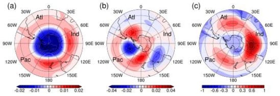
Figure 1.
The spatial pattern of (a) Southern Annular Mode (SAM), (b) Pacific-South American (PSA), (c) zonal wavenumber three (ZW3). Pac, Atl and Ind indicate the Pacific sector, Atlantic sector and Indian sector, respectively.
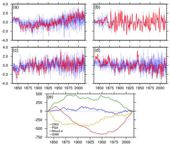
Figure 2.
The normalized index (blue dashed line) and two-year lowpass filtered index (red solid line) of (a) SAM, (b) Nino3.4, (c) PSA, (d) ZW3. (e) the cumulated index of the four.
As the most vital interannual variability signal in the ocean, ENSO has a main period of about 3–7 years, quite close to that of the ACW. The PSA induced by ENSO not only affects the climate in the tropics but also is one of the major interannual variation patterns of the atmosphere in the middle and high latitudes of the SH. In this study, the ENSO activities are characterized by the Nino3.4 index. The Nino3.4 index, which is calculated in this research based on the 20CRV3 dataset, is significantly correlated with that provided by NOAA, and the correlation coefficient is 0.85 (p < 0.01), indicating that this calculated index is applicable to this study. Similar to the SAM index series, a low-pass Lanczos filter was also conducted on the Nino3.4 index series to obtain the low-frequency signals for a period of more than two years (Figure 2b). Moreover, the cumulative values of the filtered Nino3.4 index series were calculated, as shown in Figure 2e. The results indicate that the filtered Nino3.4 index shows a significant multi-year periodic oscillation with a mutation in the mid-to-late 1870s, as confirmed by the Mann–Kendal test. Specifically, the Nino3.4 index has a significantly increasing trend before the mutation while a marked decreasing trend after that. Three dominant phase transitions can be found from the cumulative values of the filtered Nino3.4 index series. During the 1840s–1870s, 1890s–1910s and 1980s–2000s, the cumulative index values tended to increase, suggesting that the filtered Nino3.4 index values were dominated by positive values during these periods, while the situation in the remaining periods shows a decreasing trend with mainly negative values.
The PSA is a pattern in the SH corresponding to the Pacific-North American teleconnection in the Northern Hemisphere, first proposed by Mo and Ghil [34] and then Karoly [35] in an analysis of winter anomalies of ENSO events, which is a teleconnection pattern associated with ENSO. This pattern appears on wide time scales from daily to decadal, and it is one of the most dominant patterns in the SH atmosphere. In this paper, the PSA index is calculated by the method provided by the CB01 [8]. An EOF analysis was carried out for monthly geopotential height anomalies at 500 hPa (Figure 1b), and the time series of the second pattern was taken as the PSA index series. In addition, a low-pass Lanczos filter was performed on this PSA index series for low-frequency signals for a period of more than two years (Figure 2c). The filtered PSA index shows an overall upward trend. The characteristics of multi-year oscillations occur around 1900 and the latter half of the 20th century, especially in the 1960s and 1990s, when the amplitude is relatively large. The cumulative values of the filtered PSA index indicate that the PSA is dominated by negative values until the 1870s, with alternating positive-negative oscillations during the 1870s–1910s, a positive phase during the 1920s–1950s, alternating positive-negative oscillations during the 1960s–1990s, and a positive phase after 2000 (Figure 2e).
The zonal wavenumber three (ZW3) is a primary atmospheric pattern in the SH. It appears in a standing three-wave structure in the middle and high latitudes, with time scales ranging from daily to interdecadal [36]. The ZW3 index used in this research can be calculated by the method from Cerrone [9]. That is, a single point correlation was performed on monthly SLP anomaly fields with the reference point (50° S, 96° E), and the two maximum values of the positive correlation coefficient appeared at the points of 48° S, 156° W and 45° S, 5° W (Figure 1c). The arithmetic mean of the monthly SLP anomalies at these three points was defined as the ZW3 index. Similarly, the low-pass Lanczos filter was performed on this ZW3 index series, and the cumulative values of the ZW3 index were also calculated (Figure 2d,e). The filtered ZW3 index shows an overall downward trend, with temporary upward trends in the 1850s–1870s, 1920s–1940s and the early 21st century. The cumulative values of the ZW3 index declined rapidly from the 1950s to the 1990s, indicating that the values are mainly negative in this period. Especially, since the 1980s, the decline accelerates, corresponding to a larger negative ZW3 index.
4. Results
4.1. Results of the Sea Level Pressure
The spatial pattern and time series of the first four EOF patterns of the SLP (SLPEOF 1–4, SLPPC 1-4) are shown in Figure 3. The four patterns contribute 31.4%, 19.5%, 11.2% and 8.8% of the total variance, respectively. The first spatial pattern shows a near concentric structure with positive values at high latitudes and negative values at mid-latitudes (Figure 3a). Although it is approximately uniform in latitudinal direction, there is a strong large-value center in the middle of the South Pacific and a secondary large-value center in the Indian Ocean sector, resulting in a wavenumber-2 structure in the ACW area. This opposite distribution of the SLP at high and low latitudes is quite similar to the SAM pattern calculated above. Therefore, we regress the anomalies at 850 hPa in the south of 20° S on the time series of the SLPEOF 1. The regressive pattern shows a similar distribution to the SAM pattern (of the opposite sign), with only one difference: the large-value centers in the middle of the South Pacific and the West Indian Ocean sector in high latitudes are enhanced, which leads to an ACW-2 pattern in the Sub-Antarctic Zone (Figure omitted). PC of the SLPEOF 1 shows a significant interannual oscillation, with an obvious interdecadal variation (Figure 3e). Its amplitude exceeds one standard deviation, mainly during the 1880s–1890s, 1920s–1930s and 1950s–1970s, and reaches the maximum in the 1980s and 1990s. In addition, the correlation coefficient between the SLPPC 1 and the filtered SAM index is -0.26 (p < 0.01), implying that there is a strong connection between this pattern and the SAM. The SLPEOF 2 has positive loadings in the South Pacific and negative loadings in the Atlantic (Figure 3b), exhibiting a distinctive PSA pattern similar to the 500 hPa geopotential height distribution of the CB01 [8] and Simmonds and King [37]. The SLPPC 2 has the same stable interannual oscillation characteristics as the filtered PSA index during the 1960s–1990s (Figure 3f), and they also have a strong correlation, with a correlation coefficient of −0.45 (p < 0.01). The SLPEOF 3 has three positive centers in the mid-latitudes in the mid-Pacific, the Indian Ocean and the Atlantic Ocean, respectively, resulting in an ACW-3 pattern in this area. The positive centers are close to the three reference points for calculating the ZW3 index, which confers a ZW3 pattern. The time series of the SLPEOF 3 also shows large fluctuations in the 1920s, 1940s and 1970s, corresponding to brisk ZW3 activities, and its correlation coefficient with the filtered ZW3 index is 0.31 (p < 0.01), implying a covariation between these two. Similar to the SLPEOF 3, the SLPEOF 4 also has three positive centers in the ACW area, but the center positions are different, and there are large negative values in this area (Figure 3d). The SLPEOF 1 and SLPEOF 2 explain variance far beyond the SLPEOF 3 and SLPEOF 4, indicating that the ACW-2 is more dominant than the ACW-3 for the SLP. These four EOFs contribute more than 70% of the total variance. Hence, these four patterns are selected for reconstructing the ACW.
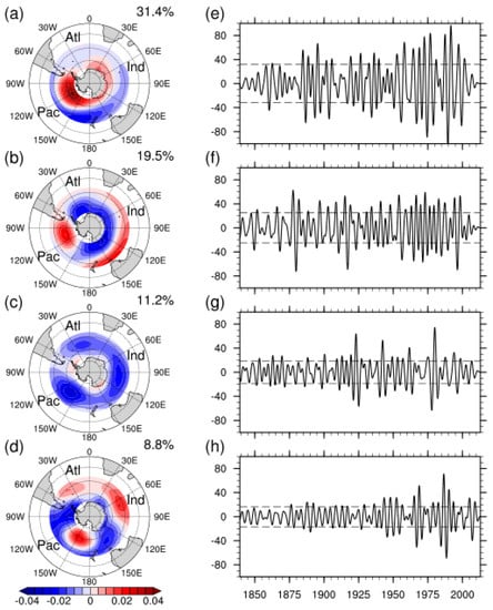
Figure 3.
The first four EOF (a–d) spatial patterns and (e–h) time series of the filtered SLP anomalies with the explained percentage of variance given on the top right of spatial patterns (contours at an interval of 0.005 hPa per unit of time series). The dashed horizontal lines in the time series denote the thresholds of one standard deviation.
Figure 4 shows the time-longitude diagram of the reconstructed SLP signal. Compared with the initial filtering result, the eastward-propagating ACW is enhanced in the amplitude in the 1980s and 1990s, which is consistent with the results of the WP96 [1] (nearly 5 hPa amplitude). The signal is not evenly distributed in the latitudinal direction. Specifically, the area with the largest amplitude is located near the Drake Passage in the South Pacific, which consists of Lin and Bian [26], coinciding with the strong center of the SLPEOF 1. However, the amplitude in the southern Indian Ocean is not significant. This variation persists over time. A shortcoming of the reconstructed signal is that a fuzzy quasi-standing wave appears in the Indian Ocean sector instead of a propagating signal. This phenomenon also can be found in previous research based on reanalysis data [9,26,38]. There is a controversy that the ACW is a standing wave rather than a propagating wave in the Indian Ocean sector [39]. Additionally, the SLP signal can be divided into four different phases in terms of amplitude variations. Specifically, the first phase is the years before the 1870s, when there are few anomalies to identify the ACW signal. The second phase is the years between the 1870s and 1940s when weak eastward-propagating anomalies can occasionally be found. For example, weak eastward-propagating anomalies are found during 1915–1930 in the South Pacific, although the consistency of the eastward propagation is partially interrupted. The most significant ACW appears in the third phase of the 1950s–1990s, and the ACW amplitude gradually disappears in the fourth phase of the 21st century. Note that a large anomaly appears in the late 1970s, without propagating eastward.
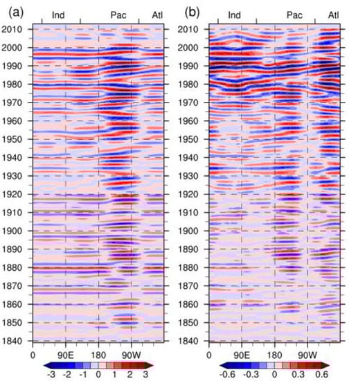
Figure 4.
Time-longitude (Hovmöller) diagrams of the reconstructed (a) sea level pressure (SLP) (contours at 0.5 hPa interval) and (b) sea surface temperature (SST) (contours at 0.1 K interval).
Several previous works have mentioned the interdecadal change in the ACW periodicity during the 1970s. However, there are different opinions about the period characteristics of the ACW before and after the trend shift. Some suggested that the period becomes shorter after the trend shift [38], while others found the opposite [9,25]. We think the contradiction comes from the methods used to calculate the ACW period. In previous studies, the average ACW period was calculated by dividing one time period by the ACW numbers passing in the time-longitude diagram before and after the trend shift. This method relies mainly on subjective identifications to distinguish ACWs, which is not an accurate estimate [39]. Moreover, the poor continuity of the eastward-propagating signal makes the numbers of ACWs counted inconsistent, resulting in discrepancies in results. The results from this research indicate that the eastward-propagating characteristics of the ACW are more consistent after the trend shift with increased fluctuation amplitude, while the change in period is not significant. Considering the interdecadal variability of the SLPEOF 1–4 mentioned above, we propose that the leading cause is the strength variation of the ACW-2 pattern. The filtered SAM index is mainly positive after 1950, and its sudden increase after the mid-1970s leads to the enhancement of the SLPEOF 1 because the positive SAM phase represents the strengthening of the sub-Antarctic westerly wind which provides the circulation in favor of the east-propagating ACW [26]. Meanwhile, the pronounced SLPEOF2 amplitude is associated with the intensification of the PSA interannual oscillation, which may be a secondary cause. Note, however, that the filtered SAM index is also mainly positive during the 1840s–1850s, while an active SLPEOF 1 is not found, suggesting that the SAM index cannot fully explain the interdecadal differences in the SLPEOF 1 and may only indicate the dynamic factor [26]. In addition, since the ACW reconstruction method based on the EOF analysis removed unexpected signals to enhance the anomalies in this study, the ACW signal is more evident than that obtained by using filters alone, which is more suitable for long-term ACW research.
4.2. Results of the Sea Surface Temperature
The first four EOF patterns of the SST (SSTEOF 1–4) contribute 18.2%, 13.4%, 9.4% and 6.1% of the total variance, respectively, with a total variance contribution of more than 47% (Figure 5a–d). The contribution rate is lower than that of the SLP and CB01, where 17 years of SST data were investigated in the CB01 [8]. However, since the research period is 180 years in this study, these patterns still dominate the ACW, suggesting a more complicated situation for the SST than the SLP. The SSTEOF 1 has positive centers in the South Pacific and the Indian Ocean, with negative loadings and an ACW-2 structure. Similar to the result in the CB01 [8], this pattern may be able to identify ENSO, although the equatorial zone is not shown. The time series of the SSTEOF 1 also has an apparent interdecadal variation (Figure 5e). Its amplitude exceeds one standard deviation, mainly after 1970, corresponding to the turn in the dominant phase of the filtered Nino3.4 index. Furthermore, during the 1980s–1990s, when the ACW is most active, SSTPC 1 has outstanding negative values in 1980, 1987, 1992 and 1998, corresponding to four El Niño events, which implies a correlation between this pattern and ENSO. The correlation coefficient between SST PC1 and the filtered Nino3.4 index is 0.48 (p < 0.01), supporting this hypothesis. However, it should be admitted that the interdecadal variation of the filtered Nino3.4 index near 1900 is not reflected in SSTPC 1, indicating that ENSO is one but not the only factor that induces this pattern.
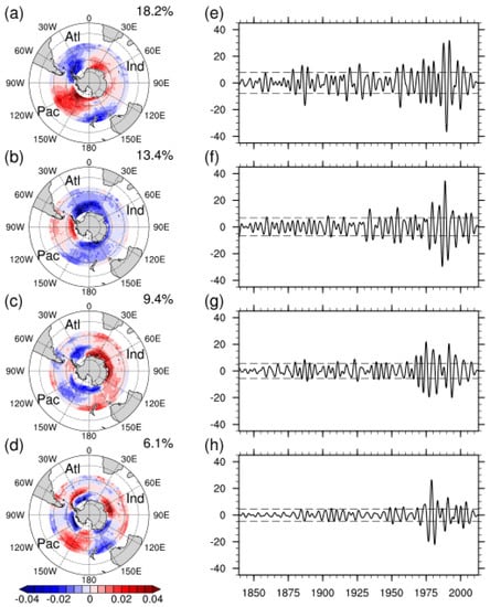
Figure 5.
The first four EOF (a–d) spatial patterns and (e–h) time series of the filtered SST anomalies with the explained percentage of variance given on the top right of spatial patterns (contours at an interval of 0.005 K per unit of time series). The dashed horizontal lines in the time series denote the thresholds of one standard deviation.
The SSTEOF 2 is confusing, with only one distinct positive center near the Drake Passage in the South Pacific, which is consistent with one of two positive centers in SSTEOF 3 for the CB01 [8]. In the Indian Ocean sector, where a second positive center is supposed to appear, a small negative value of approximately 0 appears in our results, thus breaking the ACW-2 structure. The SSTEOF 1 and 3 in the CB01 reflect the ENSO influence on the ACW, differing in that they have about 90° out of phase [8]. Calculating the time lag coefficient of SSTPC1 and SSTPC 2, we found the most significant correlation of 0.52 (p < 0.01) occurred at the lag of 14 months, which is consistent with their finding. In addition, the discordance mentioned above refers to the situation where the reconstructed SLP signal is not significant. Moreover, the contribution to total variance is less in the southern India sector [28], and the SST signal of the ACW is fuzzier in this area than in other sectors [40]. Previous studies have suggested that the ACW in the southern India sector moved northeastward into the subtropical region after 1977 due to the interdecadal variation of ENSO [13]. To interpret this finding, we regress the SST field in 0° S–70° S on SSTPC 2. The result indicates that the missing positive center in the SSTEOF 2 returns to the high latitudes of about 30° S near Australia (Figure omitted). SSTPC 2 has an increased amplitude after the middle and late 1970s, consistent with the interdecadal variation of the filtered Nino3.4 index (Figure 5f). The SSTEOF 3 and 4 show a ZW3 structure, although the loadings in SSTEOF 3 in the Indian center are fuzzy and break the ACW-3 structure. Their time series also has the approximate 90° lag phase as the situation of the SSTEOF1 and SSTEOF 2, with the most significant correlation coefficient of 0.47 (p < 0.01) at the lag of 15 months (Figure 5g,h). These two patterns were mainly active in the 1970s–1990s.
Similar to the SLP reconstruction, the SST signal is reconstructed by the first four EOF patterns, and the time-longitude diagram is shown in Figure 4. During the 1980s–1990s when the ACW signal is most pronounced, the fluctuation amplitude is about 1 K, more significant than the initial filtered signal and consistent with the results of WP96 and CB01 [1,8]. The latitudinal intensity variation is consistent with that of the SLP, with the largest near the Drake Passage and the smallest in the southern India sector. During the past 180 years, there is also an interdecadal variation of the SST signal of the ACW, and it is divided into four phases. Specifically, the first phase is the years before the mid-1870s, when there are few anomalies to identify the ACW signal. The second phase is the 1880s–1970s when the ACW is partially present both regionally and temporally. For example, it can be found that the strong anomalies propagate eastward in the South Pacific and Atlantic in the late 1880s and the whole 1950s. The most significant propagating signal appears in the third phase of the 1970s–1990s. After 2000, i.e., in the fourth phase, the SST anomalies weaken rapidly. Considering the interdecadal variation of each pattern, we suppose that the strengthening of the SST signal after the mid-1970s is contributed by both the ACW-2 and ACW-3, and the interdecadal variation of ENSO causes the shift of the ACW-2 pattern. Additionally, the periods with the pronounced SST signal before the 1970s correspond to the vigorous activities of the SSTEOF 1, which reflects the leading role of this pattern.
4.3. SVD Results
As an ocean–atmosphere coupling system, the ACW was found to be associated with the different ocean–atmosphere variable signals as early as when it was proposed in WP96 [1]. Previous studies are mostly based on the independent ocean–atmosphere variable signals or discussed multiple signals separately, and the relationships among the different ocean–atmosphere variable signals are rarely discussed. In this study, we discuss the interdecadal variations of the SLP and SST signals, respectively, and also try to discover the correlation between them. For example, the correlation coefficient between the SLPPC 1 and SSTPC 1 reaches 0.75 (p < 0.01), and the maximum time lag correlation appears when the SLPPC 1 is three months ahead of the SSTPC 1 (correlation coefficient of 0.82, p < 0.01). Therefore, we introduced the SVD method to find the main covariance modes of the two ocean–atmosphere variables (SLP and SST) and their corresponding relationship (Figure 6).
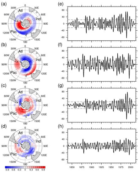
Figure 6.
The nonhomogeneous (a–d) correlation patterns and (e–h) time series of the first two SVD patterns (contours at 0.1 intervals). The dashed horizontal lines in the time series denote the thresholds of one standard deviation.
The first pair of nonhomogeneous correlation patterns explains 42.4% of the total covariance, which passed the significance test at a 90% confidence level. The spatial distribution of the first SLP nonhomogeneous correlation pattern (Figure 6a) is consistent with the SLPEOF1. That is, two positive centers appear at high latitudes, where the stronger one is located in the South Pacific, and the other is located between the Indian Ocean and the Atlantic Ocean. In such a situation, an ACW-2 pattern is formed around the pole in the middle and at high latitudes. Additionally, the corresponding time series (Figure 6e) have large amplitudes in the 1880s, 1915–1930 and 1950–1990s. Similar to the SLPEOF 1, this first SLP nonhomogeneous correlation pattern characterizes the SAM, explaining 19.1% of the SLP variance. Moreover, the corresponding first SST nonhomogeneous correlation pattern (Figure 6c) is quite similar to the SSTEOF 1 pattern, which also shows the characteristics of the ACW-2, i.e., the two positive centers are located in the South Pacific and the Indian Ocean. This pattern explains 14.5% of the SST variance. The correlation coefficient of the time series of this nonhomogeneous correlation field is 0.85, peaking at 0.87 with a lag of −2. This means, that when the SLP time series is two months ahead of the SST time series, their correlation is maximum, which is consistent with the results from the CB01 [8].
The second nonhomogeneous correlation pattern of SLP (Figure 6b), which contributes 22.7% of the variance, presents an apparent PSA pattern. It is similar to the SLPEOF 2 but has a slight eastward movement. Its time series shows that three periods with large amplitude values are also consistent with the active periods of the SLPEOF 2. The corresponding second SST nonhomogeneous correlation pattern (Figure 6d) explains 9.7% of the SST variance. A strong and a weak center occurs in the South Pacific and the Indian Ocean, respectively, and their positions move slightly eastward compared with the first SST nonhomogeneous correlation pattern. The significant difference with the SSTEOF 2 is that the second SST nonhomogeneous correlation pattern captures the weak center in the southern Indian Ocean sector and fully reveals the wavenumber-2 structure around the pole. The time-series correlation coefficient of the second pair nonhomogeneous correlation pattern is 0.81 (the maximum at a time lag of −1), explaining 30.1% of the total covariance (significant at 90% confidence level).
The SVD analysis results demonstrate that the dominant patterns of the two ocean–atmosphere variables (SST and SLP) are the circumpolar 2-wave patterns, which are highly reconciled. The SLP signal is 1–2 months ahead of the SST signal. We finally note that the third and fourth pairs of nonhomogeneous correlation patterns have a 3-wave structure and explain a small proportion of the total covariance, which fail to pass the Monte Carlo test.
5. Conclusions and Discussion
As a large-scale ocean–atmosphere coupling system in the SH, the ACW significantly affects the global climate. Investigating the interdecadal variation of the ACW and finding its causes is beneficial to improving our understanding of its dynamics and climate prediction capability. In this study, we investigated the atmospheric (SLP) and oceanic (SST) aspects of the ACW from 1836 to 2015 based on the latest high-quality 20CRV3 dataset. We extracted the relevant components of the ACW-2 and ACW-3, reconstructed the ACW signal during the past 180 years, and revealed its interdecadal variation. The possible factors of interdecadal variation were also discussed based on the large-scale climate indices corresponding to each pattern. The main findings are as follows.
- The ACW signal can be linearly decomposed into the ACW-2 and ACW-3 components, with the ACW-2 pattern dominating.
- The ACW-2 pattern for the SLP is associated with the SAM and PSA, while the SST is mainly affected by ENSO. The ACW-2 signal in the SLP is ahead of that in the SST by approximately 1–2 months.
- The ACW is most significant in the South Pacific, while it is most fuzzy in the southern Indian Ocean.
- The ACW is not persistent in SLP and SST fields from 1836 to 2015 and has remarkable interdecadal variation. The fluctuation amplitude of the ACW is weak, which cannot distinguish the ACW signal from the background disturbance before the 1870s. During the 1880s–1940s, part of the east-propagating SLP signal can be found intermittently in the South Pacific and Atlantic. A similar situation can be found in the 1880s–1960s for the SST. The most significant signal appears during the 1950s–1990s for the SLP and during the 1970s–1990s for the SST. Both of them weaken in the 21st century.
- The SLP has an interdecadal phase shift in the 1950s, and the amplitude strengthens thereafter. The change may be related to the interdecadal variation of the SAM and PSA associated with the ACW-2 pattern. The interdecadal phase shift of SST appears in the 1970s, which may be due to the change of ENSO.
These two variables (SLP and SST) have a lot in common. For example, both of them can be decomposed into ACW-2 and ACW-3 components, and the ACW-2 signal is dominant. However, several differences are also found between them. For instance, the total contribution of the ACW-2 and ACW-3 signals in the SLP exceeds that in SST, and the influencing factors are different. This study proposed that the SAM and ENSO are the main large-scale climate indices affecting ACW, while some pointed out that their influence is not isolated [8,9]. This is of great interest to us, and we hope to be able to compensate and reveal the mechanisms in our following work.
The changes in the SLP and SST in the 1870s are not explained by the large-scale climate indices in this research. Caution is still needed when interpreting this result because the performance of the dataset in the 19th century is still being evaluated [41]. Hence, further work using different datasets, such as CESM-LME, is welcomed for comparation. The EOF method was flawed in catching propagation signals. Other methods, such as complex EOF, could make up for shortcomings. Moreover, the view that the weakening of the ACW in the 21st century represents a new interdecadal turn is yet to be further confirmed because of the short period afterward.
Author Contributions
Z.L., T.Z. and W.Z. contributed to the conception and design of the study; Z.L. organized the database and performed the relevant analysis; Z.L. wrote the first draft of the manuscript; T.Z. contributed to manuscript revision; W.Z. and H.Z. contributed to funding acquisition; T.Z., W.Z. and H.Z. contributed to supervision. All authors have read and agreed to the published version of the manuscript.
Funding
This research was supported by the Strategic Priority Research Program of the Chinese Academy of Sciences (XDA20020201) and the National Natural Science Foundation of China (41675072, 41975115, 41922033).
Institutional Review Board Statement
Not applicable.
Informed Consent Statement
Not applicable.
Data Availability Statement
Publicly available datasets were analyzed in this study. This data can be found at: https://legacy.bas.ac.uk/met/READER/surface/stationpt.html (accessed on 1 March 2022), https://psl.noaa.gov/data/gridded/data.20thC_ReanV3.html (accessed on 1 March 2022), and https://psl.noaa.gov/data/20thC_Rean/timeseries/monthly/SAM/ (accessed on 1 March 2022).
Acknowledgments
Figures were produced using the NCAR Command Language (NCL).
Conflicts of Interest
The authors declare no conflict of interest.
References
- White, W.B.; Peterson, R.G. An Antarctic Circumpolar Wave in surface pressure, wind, temperature and sea-ice extent. Nature 1996, 380, 699–702. [Google Scholar] [CrossRef]
- Jacobs, G.A.; Mitchell, J.L. Ocean circulation variations associated with the Antarctic Circumpolar Wave. Geophys. Res. Lett. 1996, 23, 2947–2950. [Google Scholar] [CrossRef]
- Bonekamp, H.; Sterl, A.; Komen, G.J. Interannual variability in the Southern Ocean from an ocean model forced by European Centre for Medium-Range Weather Forecasts reanalysis fluxes. J. Geophys. Res. Earth Surf. 1999, 104, 13317–13331. [Google Scholar] [CrossRef]
- Yuan, X.; Martinson, D.G. Antarctic Sea Ice Extent Variability and Its Global Connectivity. J. Clim. 2000, 13, 1697–1717. [Google Scholar] [CrossRef]
- Christoph, M.; Barnett, T.P.; Roeckner, E. The Antarctic Circumpolar Wave in a Coupled Ocean–Atmosphere GCM. J. Clim. 1998, 11, 1659–1672. [Google Scholar] [CrossRef]
- Cai, W.; Baines, P.G.; Gordon, H.B. Southern Mid- to High-Latitude Variability, a Zonal Wavenumber-3 Pattern, and the Antarctic Circumpolar Wave in the CSIRO Coupled Model. J. Clim. 1999, 12, 3087–3104. [Google Scholar] [CrossRef]
- White, W.B.; Cayan, D.R. A global El Niño-Southern Oscillation wave in surface temperature and pressure and its interdecadal modulation from 1900 to 1997. J. Geophys. Res. Earth Surf. 2000, 105, 11223–11242. [Google Scholar] [CrossRef]
- Cai, W.; Baines, P.G. Forcing of the Antarctic Circumpolar Wave by El Niño-Southern Oscillation teleconnections. J. Geophys. Res. Earth Surf. 2001, 106, 9019–9038. [Google Scholar] [CrossRef]
- Cerrone, D.; Fusco, G.; Cotroneo, Y.; Simmonds, I.; Budillon, G. The Antarctic Circumpolar Wave: Its Presence and Interdecadal Changes during the Last 142 Years. J. Clim. 2017, 30, 6371–6389. [Google Scholar] [CrossRef]
- Venegas, S.A. The Antarctic Circumpolar Wave: A Combination of Two Signals? J. Clim. 2003, 16, 2509–2525. [Google Scholar] [CrossRef]
- Wang, X.; Giannakis, D.; Slawinska, J. The Antarctic Circumpolar Wave and its seasonality: Intrinsic travelling modes and El Niño-Southern Oscillation teleconnections. Int. J. Clim. 2018, 39, 1026–1040. [Google Scholar] [CrossRef]
- Zhou, Q.; Zhao, J.; He, Y. Review of Studies of the Antarctic Circumpolar Wave. Adv. Earth Sci. 2004, 19, 761–766. (In Chinese) [Google Scholar] [CrossRef]
- White, W.B. Influence of the Antarctic Circumpolar Wave on El Niño and its multidecadal changes from 1950 to 2001. J. Geophys. Res. Earth Surf. 2004, 109, C06019. [Google Scholar] [CrossRef]
- White, W.B.; Cherry, N.J. Influence of the Antarctic Circumpolar Wave upon New Zealand Temperature and Precipitation during Autumn–Winter. J. Clim. 1999, 12, 960–976. [Google Scholar] [CrossRef]
- White, W.B. Tropical Coupled Rossby Waves in the Pacific Ocean–Atmosphere System. J. Phys. Oceanogr. 2000, 30, 1245–1264. [Google Scholar] [CrossRef]
- Xie, J.P.; Guo, P.W.; Wang, Y.L. Antarctic Circumpolar Waves and Its Association with the Abnormality of Summer Rainfall over China. J. Nanjing Inst. Meteorol. 2005, 28, 376–383. (In Chinese) [Google Scholar] [CrossRef]
- Prabhu, A.; Mahajan, P.N.; Khaladkar, R.M.; Chipade, M.D. Role of Antarctic Circumpolar Wave in modulating the extremes of Indian summer monsoon rainfall. Geophys. Res. Lett. 2010, 37, L14106. [Google Scholar] [CrossRef]
- Huang, N.E.; Shen, Z.; Long, S.R.; Wu, M.C.; Shih, H.H.; Zheng, Q.; Yen, N.-C.; Tung, C.C.; Liu, H.H. The empirical mode decomposition and the Hilbert spectrum for nonlinear and non-stationary time series analysis. Proc. R. Soc. Lond. Ser. A Math. Phys. Eng. Sci. 1998, 454, 903–995. [Google Scholar] [CrossRef]
- Comiso, J.C. Variability and Trends in Antarctic Surface Temperatures from In Situ and Satellite Infrared Measurements. J. Clim. 2000, 13, 1674–1696. [Google Scholar] [CrossRef]
- Cerrone, D.; Fusco, G.; Simmonds, I.; Aulicino, G.; Budillon, G. Dominant Covarying Climate Signals in the Southern Ocean and Antarctic Sea Ice Influence during the Last Three Decades. J. Clim. 2017, 30, 3055–3072. [Google Scholar] [CrossRef]
- Moroi, T.; Kitoh, A.; Koide, H. Antarctic Circumpolar Wave in a coupled ocean-atmosphere model. Ann. Glaciol. 1998, 27, 483–487. [Google Scholar] [CrossRef]
- Belkin, I.M. Comments on “Southern Mid- to High-Latitude Variability, a Zonal Wavenumber-3 Pattern, and the Antarctic Circumpolar Wave in the CSIRO Coupled Model”. J. Clim. 2001, 14, 1329–1331. [Google Scholar] [CrossRef]
- Cai, W.; Baines, P.G.; Gordon, H.B. Reply. J. Clim. 2001, 14, 1332–1334. [Google Scholar] [CrossRef]
- Xiao, C.; Chen, Y.; Ren, J.; Lu, L.; Li, Z.; Qin, D.; Zhou, X. Signals of Antarctic Circumpolar Wave over the Southern Indian Ocean as recorded in an Antarctica ice core. Chin. Sci. Bull. 2005, 50, 347–355. [Google Scholar] [CrossRef]
- Bian, L.; Lin, X. Interdecadal change in the Antarctic Circumpolar Wave during 1951–2010. Adv. Atmos. Sci. 2012, 29, 464–470. [Google Scholar] [CrossRef]
- Lin, X.; Bian, L. Characteristics of the Antarctic Circumpolar Wave during Recent 100 Years. Clim. Environ. Res. 2015, 20, 21–29. (In Chinese) [Google Scholar]
- Gloersen, P.; Huang, N.E. In search of an elusive Antarctic Circumpolar Wave in sea ice extents: 1978–1996. Polar Res. 1999, 18, 167–173. [Google Scholar] [CrossRef]
- Giarolla, E.; Matano, R.P. The Low-Frequency Variability of the Southern Ocean Circulation. J. Clim. 2013, 26, 6081–6091. [Google Scholar] [CrossRef][Green Version]
- Slivinski, L.C.; Compo, G.P.; Whitaker, J.S.; Sardeshmukh, P.D.; Giese, B.S.; McColl, C.; Allan, R.; Yin, X.; Vose, R.; Titchner, H.; et al. Towards a more reliable historical reanalysis: Improvements for version 3 of the Twentieth Century Reanalysis system. Q. J. R. Meteorol. Soc. 2019, 145, 2876–2908. [Google Scholar] [CrossRef]
- Turner, J.; Colwell, S.R.; Marshall, G.J.; Lachlan-Cope, T.A.; Carleton, A.M.; Jones, P.D.; Lagun, V.; Reid, P.A.; Iagovkina, S. The SCAR READER Project: Toward a High-Quality Database of Mean Antarctic Meteorological Observations. J. Clim. 2004, 17, 2890–2898. [Google Scholar] [CrossRef]
- Prohaska, J.T. A Technique for Analyzing the Linear Relationships between Two Meteorological Fields. Mon. Weather Rev. 1976, 104, 1345–1353. [Google Scholar] [CrossRef]
- Thompson, D.W.J.; Wallace, J.M. Annular Modes in the Extratropical Circulation. Part I: Month-to-Month Variability. J. Clim. 2000, 13, 1000–1016. [Google Scholar] [CrossRef]
- Gong, D.; Wang, S. Definition of Antarctic Oscillation index. Geophys. Res. Lett. 1999, 26, 459–462. [Google Scholar] [CrossRef]
- Mo, K.C.; Ghil, M. Statistics and Dynamics of Persistent Anomalies. J. Atmos. Sci. 1987, 44, 877–902. [Google Scholar] [CrossRef]
- Karoly, D.J. Southern Hemisphere Circulation Features Associated with El Niño-Southern Oscillation Events. J. Clim. 1989, 2, 1239–1252. [Google Scholar] [CrossRef]
- Mo, K.C.; White, G.H. Teleconnections in the Southern Hemisphere. Mon. Weather Rev. 1985, 113, 22–37. [Google Scholar] [CrossRef]
- Simmonds, I.; King, J.C. Global and hemispheric climate variations affecting the Southern Ocean. Antarct. Sci. 2004, 16, 401–413. [Google Scholar] [CrossRef]
- Bian, L.; Lin, X. Interdecadal change of the Atlantic oscillation and the Antarctic Circumpolar Wave. Chin. J. Atmos. Sci. 2009, 33, 251–260. (In Chinese) [Google Scholar]
- Li, Y.; Zhao, J. A study on the Antarctic circumpolar wave mode-A coexistence system of standing and traveling wave. Chin. J. Polar Sci. 2006, 17, 100–110. [Google Scholar]
- Mélice, J.-L.; Lutjeharms, J.R.E.; Goosse, H.; Fichefet, T.; Reason, C.J.C. Evidence for the Antarctic circumpolar wave in the sub-Antarctic during the past 50 years. Geophys. Res. Lett. 2005, 32, L14614. [Google Scholar] [CrossRef]
- Slivinski, L.C.; Compo, G.P.; Sardeshmukh, P.D.; Whitaker, J.S.; McColl, C.; Allan, R.J.; Brohan, P.; Yin, X.; Smith, C.A.; Spencer, L.J.; et al. An Evaluation of the Performance of the Twentieth Century Reanalysis Version 3. J. Clim. 2021, 34, 1417–1438. [Google Scholar] [CrossRef]


Publisher’s Note: MDPI stays neutral with regard to jurisdictional claims in published maps and institutional affiliations. |
© 2022 by the authors. Licensee MDPI, Basel, Switzerland. This article is an open access article distributed under the terms and conditions of the Creative Commons Attribution (CC BY) license (https://creativecommons.org/licenses/by/4.0/).