Abstract
A multimodel superensemble technique was applied to improve the accuracy of a model predicting the subseasonal surface air temperatures in East Asia. Superensemble forecast data based on seven subseasonal-to-seasonal (S2S) forecast models were produced for the initial times from May to August in 2016–2020 and forecast days in weeks 1–4. Superensemble techniques based on the root-mean-square error ensemble mean (SUPR) and the linear regression coefficient ensemble mean (SUPL) were evaluated and compared with the forecast bias-removed ensemble mean (ENS) data. The magnitudes of the forecasting root-mean-square errors (RMSE) of the SUPR and SUPL methods were 4.2% and 13.8% lower, respectively, than that of the ENS method, and the most significant effect was in 2020. The RMSE improvements of SUPR and SUPL were high when the initial date was in May, June, and August, and the forecast date was within weeks 1–4. Applying multimodel superensemble methods effectively reduced the forecasting errors of the S2S models. If weight coefficients based on the characteristics of the models are appropriately applied, the forecasting performance can be significantly improved.
1. Introduction
The duration and intensity of heatwaves have significantly increased in recent years, and damages from heatwaves are expected to increase owing to global warming [1,2]. An increase in the number of high-temperature days can cause various socioeconomic effects, such as a decrease in agricultural production and an increase in thermal diseases. To prepare for such disasters, it is critical to accurately predict the surface air temperatures.
The subseasonal-to-seasonal (S2S) forecast project currently provides forecast data using 12 models for continuous forecasting studies, ranging seamlessly from weather to climate [3,4]. The forecasted data have been produced since 2015 and are predicted for 30–60 days from the initial date, depending on the model. These data were used for studying the Madden–Julian oscillation, typhoons, heatwaves, and stratosphere-troposphere interactions [5,6,7,8].
Climate forecasting has errors as the atmosphere is an unstable and nonlinear system. The forecasting performance of the models can be improved by modifying the source code, parameters, and boundary conditions, which require significant resources and time. Additionally, it is difficult to reduce the inherent nonlinear errors in the model. Another approach is to use multimodel ensemble techniques. If the forecasted data are produced by averaging the data of various models simulated for the same purpose, the forecast performance can be improved due to the offset of errors on unpredictable scales.
Multimodel ensemble techniques include straightforward ensemble mean, bias-removed ensemble, and error-based superensemble methods [9,10,11,12]. The straightforward ensemble is the average of all models for the forecast period. In this method, the forecasted data can be produced relatively simply and easily. However, the biases to the observation data are also included in the data. The bias-removed ensemble is an average of all models while accounting for each model’s inherent observation error for an initial date and forecast time. In this method, the models contributing to the mean have the same weight. Thus, the quality of the forecasted data can be affected by the use of models with relatively large errors. The error-based superensemble technique is an average that considers the characteristics of each model, such as root-mean-square error magnitude and regression coefficient of the model and observation. As the forecast data generated by this technique can have significantly lower forecast errors than those obtained by other techniques, this method has been used to improve errors in variables such as surface temperature, precipitation, and geopotential height [9,10,11,12,13,14,15,16]. This method was applied to East Asia from July to August 2018 [12].
The error-based superensemble technique requires a training period to calculate the weight coefficients considering the model characteristics and requires weeks to years of forecasting data. For the S2S models, the weight coefficients can be calculated using the long-term reforecast data. Consequently, it is possible to produce real-time bias-removed ensemble and error-based superensemble forecast data.
This study analyzed the error characteristics of the forecasted surface air temperatures by applying an error-based superensemble for May–August for five years (2016–2020) of real-time forecasted data from the S2S models. Two types of error-based superensemble forecast data with weight coefficients were produced using the root-mean-square error (RMSE) and linear regression of each model. The bias-removed ensemble forecast data were compared to reduce the error in predicting the surface temperatures in East Asia. Although a previous study analyzed surface air temperatures in East Asia, they only considered July–August 2018 [12]. In this study, we used statistical analyses covering several years. Using yearly, monthly, and forecasted time analyses, we determined the characteristics of the forecasting errors for each period.
2. Materials and Methods
2.1. Data
Seven models participating in the S2S forecast data project were analyzed (Table 1). Real-time data from May to August for the years 2016–2020 were used. However, ECCC and KMA data were excluded from the 2016 data due to missingness. The 1999–2010 period, for which all the models had reforecasted data, was used to calculate the weight coefficients. In addition, this study analyzed the forecast time of 1–31 days, which is a period commonly employed by all the models used in this study. The models have been described in detail by [4].

Table 1.
Brief descriptions of the selected S2S database.
Data from the models were provided at a 1.5° × 1.5° resolution. The initial time interval was daily for CMA, KMA, NCEP, and UKMO, weekly for ECCC and ISAC-CNR, and twice weekly for ECMWF. When the initial time of the model used in the analysis was matched once a week to analyze the predictability of the surface air temperature in summer, there were 17 days in total from May to August.
To evaluate the model’s predictability, the National Centers for Environmental Prediction-National Center for Atmospheric Research (NCEP/NCAR) reanalysis 2 data were used as reference data for error analysis [17]. The NCEP data showed a very high correlation with the in situ observation of surface air temperature over the Korean Peninsula (not shown). The period was the same as that of the S2S model data, and the horizontal resolution was interpolated and analyzed similarly to that of the S2S data. The study area was East Asia (25°–50° N, 105°–150° E, Figure 1f).
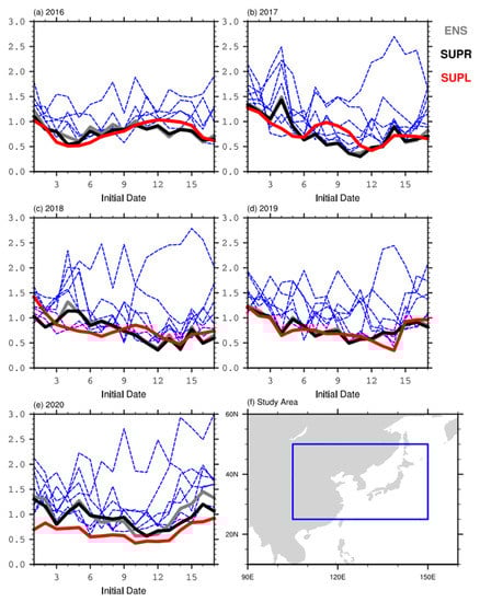
Figure 1.
Variation in the root-mean-square error (RMSE) at the initial 1–17 days, derived from seven models (blue lines) and the ensemble forecasts of ENS (grey line), SUPR (black line), and SUPL (red line) in (a) 2016, (b) 2017, (c) 2018, (d) 2019, and (e) 2020. The blue box in (f) represents the study area.
2.2. Methodology
As the forecasted data of the model contained systematic errors, a correction was required using observed data. The technique of [14,15,16] was used to generate the superensemble forecast data. The superensemble forecast data for forecast time t are defined as follows.
where is the superensemble real-time forecasted value at forecast time t, is the average observed value for the training period, is the real-time forecasted value of the ith model at the initial and forecast time t, is the average forecasted value for the training period of the ith model at initial and forecast time t, and is the weight coefficient of the ith model. The training period was 1991–2010, which was the reforecasted data period, and the real-time forecasted values corresponded to 2016–2020.
The superensemble forecast data were produced using the two methods to calculate the weight coefficients. In the first method, the RMSEs of each model and observed data for the training period were calculated, and this method was denoted as SUPR. The weight coefficient of the SUPR method () is defined as follows.
Here, the RMSE is defined as follows.
where t is the initial and forecast time for the training period. Therefore, the SUPR method can be expressed as follows.
In the second method, the linear regression coefficients of the model and observations during the training period were determined as the superensemble weight coefficient and used to calculate the weight coefficients. This method was denoted as SUPL.
While the weight coefficient of SUPR has a positive value that is calculated based on RMSE, that of SUPL can have either a positive or negative value as it is calculated based on regression analysis. Thus, if the model has a negative value according to the initial days and forecast time in the reforecast data, the coefficient is also applied to the real-time data.
To compare these two superensemble techniques, a multimodel ensemble mean (ENS) was defined as a reference, which allows all models to have the same weight.
The forecast performance of the model was compared in terms of mean bias error (MBE) and RMSE. The model forecast and observation values were denoted as M and O, respectively. The MBE and RMSE can thus be obtained using the following equations.
In both cases, the error was lower when it approached zero. MBE may be offset by the sum of the bias, but the sign of the error can be checked. In contrast, the magnitude of the total error was checked for the RMSE.
3. Results
Three sets of superensemble forecasts were obtained based on seven S2S models. Figure 1 shows the RMSE of the average surface air temperature in East Asia from 2016 to 2020, which was averaged for 1–31 days for an initial time of 1–17 days. The forecast time of 1–31 days is a period commonly employed by all the models. Each model is shown in blue dashed lines, and the ENS, SUPR, and SUPL methods are shown in grey, black, and red solid lines, respectively. The RMSEs of the individual models were in the range of 0.37 and 3.0, whereas those of the ENS, SUPR, and SUPL methods ranged between 0.30 and 1.49. Superensemble forecast data with a narrow range of errors have lower errors than the data from individual models with wider ranges of errors. The RMSE of the model can be reduced by averaging the forecast biases of the models due to the offsetting of the inherent errors of the models. As the initial time interval was 17 days from May to August, the error was small in May (1–4 days) in 2016 and in July (10–13 days) in the other years. The change in RMSE of the SUPR method was similar to that of the ENS method, and the error of the SUPR method was low. The RMSE of the SUPL method exhibited different variation characteristics from those of the ENS and SUPR methods. In 2016 and 2018, the initial 3–9 days had relatively low errors, but the error was higher thereafter. In 2020, the SUPL method had a very low error compared to the forecasts made by individual models and other superensemble techniques for all initial days.
Figure 2 is a graph of the RMSE of the average surface temperatures in East Asia from 2016 to 2020 for forecast times of 1–31 days. Similar to the results for the initial time (Figure 1), the ensemble forecast data had lower RMSEs than those of the individual models. In addition, the error correction effect of the SUPL was high in 2020. In 2018 and 2019, when the forecast time exceeded 16 days, the forecasted data of the three ensembles had similar errors when the error values of all models were high, but the SUPL method had notably lower errors when the error was small. Therefore, in the forecasts for weeks 3 and 4, the SUPL method had a higher error correction effect when the error was small. In contrast, the three ensemble results were similar when the error was high.
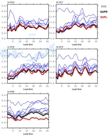
Figure 2.
Variation in RMSE at the initial 1–17 days derived from seven models (blue lines) and the ensemble forecasts of ENS (grey line), SUPR (black line), and SUPL (red line) in (a) 2016, (b) 2017, (c) 2018, (d) 2019, and (e) 2020.
The result of the RMSE time-series analysis, for both the initial time and initial days, indicates that the ensemble forecast shows superior performance over the individual models. The performance of the ensemble forecast follows that of the participating model with the lowest error but does not correlate with the model with the largest; therefore, participation of the model with the lowest error is important in an ensemble forecast. Furthermore, since the superensemble forecast data outperform simple ensemble forecast data, it is important to apply the superensemble techniques to further improve the model’s forecast performance.
The signs of the errors can be confirmed through the MBE analysis of the superensemble forecast data. Considering ENS as the model with the lowest error among the individual models, it was compared with the SUPR and SUPL forecast data to which the superensemble technique was applied. Figure 3 shows a box-and-whisker plot of the MBE of the ENS, SUPR, and SUPL forecast data for each year from 2016 to 2020. Compared with the ENS method, the maximum MBEs of the SUPR and SUPL methods were lower for all years. For 2016 and 2020, the minimum values of the SUPR and SUPL methods increased, indicating that the difference between the maximum and minimum errors had decreased. For 2017 and 2018, the MBEs of the SUPR and SUPL methods and the average MBEs were negative. These results show that the superensemble results reduce the positive bias of the model, and the effect on the negative bias correction varies annually.
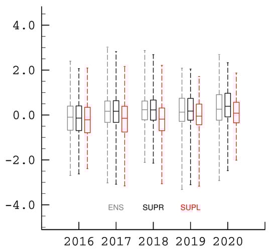
Figure 3.
Box-and-whisker plot of mean bias errors (MBEs) derived from ensemble forecast of ENS (grey), SUPR (black), and SUPL (red) for 2016–2020. The bounds of the box at the 25th and 75th percentile and the flat line in the box is the median, and the whiskers represent the minimum and maximum values.
The result of comparing ensemble data for each year showed that the range between the maximum and minimum values of the superensemble analysis data was generally reduced. The initial days were averaged for each month, and a box-and-whisker plot analysis was performed on the MBEs of ENS, SUPR, and SUPL (Figure 4). As the months are distinguished by the initial time, the actual forecast date includes the corresponding month and part of the following month. The difference between the minimum and maximum MBEs was more significant in May and August than in June and July, indicating that the error was large. The seasonal changes varied in May and August when the region was affected by high pressure in the western North Pacific. For positive bias, the MBE had small values in the order of ENS, SUPR, and SUPL. However, for the negative bias, it showed small values in the order of ENS, SUPL, and SUPR. The monthly analysis also showed that the superensemble effect reduced the positive bias. The SUPR method had a smaller negative bias, and the SUPL also had a negative bias, except for July.
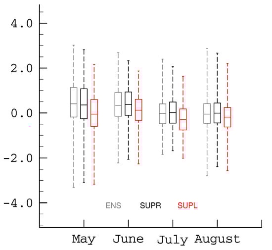
Figure 4.
Box-and-whisker plot of MBE for the initial days from May to August derived from the ensemble forecast of ENS (grey), SUPR (black), and SUPL (red). The bounds of the box are at the 25th and 75th percentile, and the flat line in the box is the median. The whiskers represent the minimum and maximum values.
The box-and-whisker plot of the MBE was created for the forecast time (Figure 5). Forecast dates 1–28 were divided into 7-day intervals and defined as weeks 1–4. An analysis by forecast time revealed that the average MBE of the ENS method was closer to zero. If the year or initial date were not considered, the ENS method showed a better forecast performance. Analysis of the bias distribution by forecast time revealed that the SUPR and SUPL methods contributed to the reduction in the width of the bias in weeks 2 and 3.
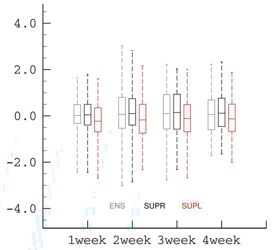
Figure 5.
Box-and-whisker plot of MBE at the 1–4 weeks, derived from the ensemble forecast of ENS (grey), SUPR (black), and SUPL (red). The bounds of the box are at the 25th and 75th percentile, and the flat line in the box is the median. The whiskers represent the minimum and maximum values.
Analysis of the bias distribution of the models showed that the SUPR and SUPL methods reduced positive bias. However, the negative bias increased on July, and in 2017 and 2018, as well as weeks 1 and 4. This effect on negative bias correction seemed to determine the MBE of the model.
The RMSEs of the ENS, SUPR, and SUPL methods from 2016 to 2020 were also analyzed (Figure 6a). The RMSE of the ENS method was approximately 0.83 from 2016 to 2019 but increased significantly to 1.03 in 2020. The SUPR and SUPL methods had errors similar to or slightly smaller than the ENS. In 2016 and 2018, the SUPR method showed better forecasting performance than the SUPL method, but in 2019 and 2020, the forecasting performance of SUPL was better. The SUPR and SUPL forecasting methods are expected to be more useful for improving the forecast performance than the ENS method.
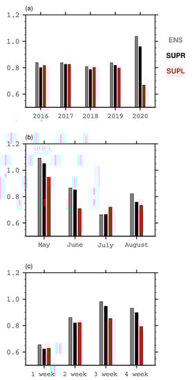
Figure 6.
RMSEs of surface air temperature for ENS, SUPR, and SUPL in (a) 2016–2020, (b) initial month from May to August, and (c) forecast time of 1–4 weeks averaged in the area of 25°–50° N, 105°–150° E.
Figure 6b shows the RMSE for the initial month under the ENS, SUPR, and SUPL methods. Except for July, the RMSE decreased in the following order: ENS, SUPR, and SUPL. In July, the RMSEs of the ENS and SUPR methods were approximately 0.66, whereas the SUPL method had the highest error at 0.72. As the forecast time was 1–31 days for the initial time of July, the predicted period corresponded to July–August.
Figure 6c presents the RMSE by forecast day for the ENS, SUPR, and SUPL methods. In weeks 1 to 3, all forecast errors increased and then decreased slightly in week 4. The SUPR and SUPL methods showed smaller RMSEs than the ENS method in all weeks, which showed a better forecast performance. In weeks 1 and 2, the SUPR and SUPL methods had similar RMSEs. However, in weeks 3 and 4, the SUPL method had lower RMSEs than the SUPR method. Therefore, for forecast dates in week 3 or later, the SUPR and SUPL forecasting methods will improve the forecast performance.
The overall RMSEs of the ENS, SUPR, and SUPL methods for 2016–2020 were 0.886, 0.848, and 0.763, respectively. The forecast errors of the SUPR and SUPL methods were 4.2% and 13.8% smaller, respectively, than those of the ENS method. The difference was most significant in 2020. Furthermore, the error improvement effect of the SUPL method was high when the initial date was in May, June, and August and when the forecast time was 1–4 weeks. These results and those presented in Figure 4, Figure 5 and Figure 6 show that the improvement in the negative bias is insignificant, or the superensemble has a larger bias when the error reduction effect is low. Therefore, if the model has a negative bias, the superensemble technique must be used more carefully.
4. Discussion
The superensemble technique was used to improve the surface air temperature forecasting performance of the S2S model in East Asia for May–August, 2016–2020. The forecast performance was improved when using ensemble techniques compared to the forecast data of individual models. The RMSE of superensemble forecast methods—SUPR and SUPL—showed decreased errors compared to those of the ENS by 4.2% and 13.8%, respectively, demonstrating that the superensemble techniques are more effective than simple ensemble forecasting in reducing the forecast errors. When comparing the SUPR and SUPL methods, the weight calculation method using linear regression coefficients showed a higher effect than using RMSEs. Meanwhile, the SUPL method showed a slightly higher error than other techniques in the initial month of July or during the great heatwave in East Asia (in 2016 and 2018). Therefore, the ENS ensemble method or the SUPR superensemble method would be more effective than the SUPL method in high-temperature cases.
Similar to the results of precedent studies, this study showed better performance in superensemble forecast means than simple ensemble results [12]. This study is important as it statistically analyzed the superensemble results by initial month and forecast time for a long period (5 years), which is longer than those considered in previous studies. The real-time forecast data spanned from 2016 to 2020, and the period of the reforecasted data with calculated weight coefficients spanned from 1999 to 2010. To reflect recent climate change, the training period should be close to the period wherein a superensemble technique is applied. Further research is needed to determine whether the forecast error can be further reduced when the weight coefficients of the superensemble are calculated using data from a period closer to the period to be predicted. More accurate results can be expected if research is conducted using forecast data obtained using a superensemble technique that considers the characteristics of individual models. The method applied in this study can be used for other periods, regions, and variables.
Author Contributions
Conceptualization, B.-K.M. and J.W.; writing—original draft preparation, J.W.; data curation, J.K.; writing—review and editing, J.W., J.K. and B.-K.M. All authors have read and agreed to the published version of the manuscript.
Funding
This study was supported by a National Research Foundation of Korea (NRF) grant funded by the Government of Korea (MSIT) (No. 2019R1A2C1008549). Jinhee Kang was supported by the National University Development Project of 2021.
Institutional Review Board Statement
Not applicable.
Informed Consent Statement
Informed consent was obtained from all subjects involved in the study.
Data Availability Statement
The following institutes produce and host the repositories of the datasets in this study: ECMWF (S2S sets, https://apps.ecmwf.int/datasets/data/s2s/, accessed on 25 March 2022), and the National Centers for Environmental Prediction (NCEP) (NCEP-DOE reanalysis 2, https://psl.noaa.gov/data/gridded/data.ncep.reanalysis2.surface.html, accessed on 25 March 2022).
Conflicts of Interest
The authors declare no conflict of interest.
References
- Almazroui, M.; Saeed, F.; Saeed, S.; Ismail, M.; Ehsan, M.A.; Islam, M.N.; Abid, M.A.; O’Brien, E.; Kamil, S.; Rashid, I.U.; et al. Projected changes in climate extremes using CMIP6 simulations over SREX regions. Earth Syst. Environ. 2021, 5, 481–497. [Google Scholar] [CrossRef]
- Campbell, S.; Remenyi, T.A.; White, C.J.; Johnston, F.H. Heatwave and health impact research: A global review. Health Place 2018, 53, 210–218. [Google Scholar] [CrossRef] [PubMed]
- Vitart, F.; Robertson, A.W.; Anderson, D.L.T. Subseasonal to Seasonal Prediction Project: Bridging the gap between weather and climate. Bull. World Meteorol. Organ. 2012, 61, 23–28. [Google Scholar]
- Vitart, F.; Ardilouze, C.; Bonet, A.; Brookshaw, A.; Chen, M.; Codorean, C.; Déqué, M.; Ferranti, L.; Fucile, E.; Fuentes, M.; et al. The subseasonal to seasonal (S2S) prediction project database. Bull. Am. Meteorol. Soc. 2017, 98, 163–173. [Google Scholar] [CrossRef]
- Baldwin, M.P.; Stephenson, D.B.; Thompson, D.W.J.; Dunkerton, T.J.; Charlton, A.J.; O’Neill, A. Stratospheric memory and extended-range weather forecasts. Science 2003, 301, 636–640. [Google Scholar] [CrossRef] [PubMed]
- Koster, R.D.; Mahanama, S.P.P.; Yamada, T.J.; Balsamo, G.; Berg, A.A.; Boisserie, M.; Dirmeyer, P.A.; Doblas-Reyes, F.J.; Drewitt, G.; Gordon, C.T.; et al. Contribution of land surface initialization to subseasonal forecast skill: First results from a multi-model experiment. Geophys. Res. Lett. 2010, 37, L02402. [Google Scholar] [CrossRef]
- Sobolowski, S.; Gong, G.; Ting, M. Modeled climate state and dynamic responses to anomalous North American snow cover. J. Clim. 2010, 23, 785–799. [Google Scholar] [CrossRef]
- Waliser, D.E. Predictability and forecasting. In Intraseasonal Variability of the Atmosphere-Ocean Climate System, 2nd ed.; Lau, W.K.M., Waliser, D.E., Eds.; Springer: Berlin/Heidelberg, Germany, 2011; ISBN 978-3-642-13913-0. [Google Scholar]
- Yun, W.T.; Stefanova, L.; Krishnamurti, T.N. Improvement of the multimodel superensemble technique for seasonal forecasts. J. Clim. 2003, 16, 3834–3840. [Google Scholar] [CrossRef]
- Zhang, H.-B.; Zhi, X.-F.; Chen, J.; Wang, Y.-N.; Wang, Y. Study of the modification of multi-model ensemble science for tropical cyclone forecasts. J. Trop. Meteorol. 2015, 21, 389–399. [Google Scholar]
- Zhi, X.; Qi, H.; Bai, Y.; Lin, C. A comparison of three kinds of multimodel ensemble forecast techniques based on the TIGGE data. Acta Meteorol. Sin. 2012, 26, 41–51. [Google Scholar] [CrossRef]
- Zhu, S.; Zhi, X.; Ge, F.; Fan, Y.; Zhang, L.; Gao, J. Subseasonal forecast of surface air temperature using superensemble approaches: Experiments over Northeast Asia for 2018. Weather Forecast. 2021, 36, 39–51. [Google Scholar] [CrossRef]
- Cartwright, T.J.; Krishnamurti, T.N. Warm season mesoscale superensemble precipitation forecasts in the southeastern United States. Weather Forecast. 2007, 22, 873–886. [Google Scholar] [CrossRef]
- Krishnamurti, T.N.; Kishtawal, M.; LaRow, T.E.; Bachiochi, D.R.; Zhang, Z.; Williford, C.E.; Gadgil, S.; Surendran, S. Improved weather and seasonal climate forecasts from multimodel superensemble. Science 1999, 285, 1548–1550. [Google Scholar] [CrossRef] [PubMed]
- Krishnamurti, T.N.; Surendran, S.; Shin, D.W.; Correa-Torres, R.J.; Vijaya Kumar, T.S.V.; Williford, E.; Kummerow, C.; Adler, R.F.; Simpson, J.; Kakar, R.; et al. Real-time multianalysis–multimodel superensemble forecasts of precipitation using TRMM and SSM/I products. Mon. Weather Rev. 2001, 129, 2861–2883. [Google Scholar] [CrossRef][Green Version]
- Krishnamurti, T.N.; Rajendran, K.; Vijaya Kumar, T.S.V.; Lord, S.; Toth, Z.; Zou, X.; Cocke, S.; Ahlquist, J.E.; Navon, I.M. Improved skill for the anomaly correlation of geopotential heights at 500 hPa. Mon. Weather Rev. 2003, 131, 1082–1102. [Google Scholar] [CrossRef]
- Kanamitsu, M.; Ebisuzaki, W.; Woollen, J.; Yang, S.-K.; Hnilo, J.J.; Fiorino, M.; Potter, G.L. NCEP-DOE AMIP-II reanalysis (R-2). Bull. Am. Meteorol. Soc. 2002, 83, 1631–1644. [Google Scholar] [CrossRef]


Publisher’s Note: MDPI stays neutral with regard to jurisdictional claims in published maps and institutional affiliations. |
© 2022 by the authors. Licensee MDPI, Basel, Switzerland. This article is an open access article distributed under the terms and conditions of the Creative Commons Attribution (CC BY) license (https://creativecommons.org/licenses/by/4.0/).