Article

Deep Learning for Predicting Winter Temperature in North China

1
School of Atmospheric Science, Nanjing University of Information Science and Technology, Nanjing 210044, China
2
Department of Oceanography, Chonnam National University, Gwangju 61186, Korea
*
Author to whom correspondence should be addressed.
Atmosphere 2022, 13(5), 702; https://doi.org/10.3390/atmos13050702
Submission received: 11 March 2022 / Revised: 18 April 2022 / Accepted: 26 April 2022 / Published: 28 April 2022
(This article belongs to the Section Climatology)

Abstract

:
It is difficult to improve the seasonal prediction skill of winter temperature over North China, owing to the complex dynamics of East Asian winter and the relatively low prediction skill level of current climate models. Deep learning (DL) may be an informative and promising tool to enhance seasonal prediction, particularly in regions where the underlying mechanisms are not clear. Here, using a DL model based on the Convolutional Neural Network (CNN), we have found that the prediction skill for North China winter temperature (NCWT) can be extended up to five months by considering the remote impact of the Northeast Pacific sea-surface temperature (SST) on North China. Based on historical simulations of winter temperatures in North China, we selected six CMIP5 models with relatively small deviations for training the CNN, and the period chosen for training was 1852–1991. The ERA5 data during 1995–2017 were utilized to evaluate the performance of the CNN. Our CNN shows the best performance in a recent 10-year period (2008–2017), showing a significantly improved level of NCWT prediction skill with a correlation skill of 0.65 at a 5-month lead time, which is much better than the forecast skill of the state-of-the-art dynamic seasonal prediction system. Heat map analysis was used to explore the possible physical mechanisms associated with the NCWT anomaly from the perspective of the CNN; the results showed that the SST over the Northeast Pacific is highly relevant to NCWT prediction. The Northeast Pacific warming in the boreal summer is related to the development of the El Niño event in the coming winter, which may induce NCWT anomalies by atmospheric teleconnection. Climate model experiments support the role of Northeast Pacific warming in the boreal summer on NCWT. The improved capability for prediction from using the CNN may help to establish the energy policy for the coming winter and reduce the economic losses from extremely cold in North China.

1. Introduction

North China has experienced several severe winter seasons during the last 10 years, with an anomalous cold winter in 2011–2012 [1], a 30-year-record cold period in the early winter of 2012–2013 [2], and severe cooling events caused by cold surges in the early winter during 2020–2021 [3]. Mild temperatures ensure that winter wheat—planted mainly in North China—is able to grow safely. The outbreak of the global pandemic COVID-19 has aroused public attention to the early warning of infectious diseases, as a negative winter temperature anomaly may be favorable for the spread of the virus [4]. Improved seasonal prediction of winter temperatures, due to its positive impact on the economy, society, public health, and energy deployment, is important [5,6].
Previous studies revealed that the winter temperature over North China may be affected by remote sea-surface temperature (SST) forcing. Serving as the strongest signal of interannual climate variability in the tropical Pacific, El Niño and Southern Oscillation (ENSO) plays an important role in the winter temperature anomaly of China. An El Niño event can lead to a warm winter climate in China, while a La Niña can lead to a cold winter [7]. On the other hand, interannual SST anomalies in the tropical Indian Ocean can induce a Pacific–North American (PNA) type of winter teleconnection in the mid and high latitudes, which has a significant influence on the winter temperature anomaly in China [8]. Other studies suggested that the Kuroshio region is the key area affecting winter temperature in China [9,10]. The Atlantic Multidecadal Oscillation (AMO) and Pacific Decadal Oscillation (PDO) also provide interdecadal background for the long-term variation of winter temperature in China and affect winter temperature through the modulation of the interannual factors. The intensity of the East Asian Winter Monsoon (EAWM) and ENSO tends to be weaker than normal when the AMO is in its warming phase; the Aleutian Low and Mongolia High (east Siberian High) tends to be strengthened (weakened) when the PDO is in its warming phase [11,12].
Although previous studies emphasized the importance of the remote impact from various climate variabilities, such remote factors are not used for the seasonal prediction of winter temperature over North China. Two dominant modes of air temperature variability over the EAWM region were identified [13], namely, the northern and southern modes. The two dominant modes can explain a significant amount of temperature variability over the entire Asia region [14]. A subtropical North Pacific–Gulf of Alaska dipole signal of SST is a significant precursor of the northern mode, which reaches its peak in the prior summer [15]. Four precursors in the prior boreal summer were selected to predict the winter temperature over China by using the Ensemble Canonical Correlation (ECC), with an unsatisfactory result occurring in North China, showing a sharp contrast with the other regions [16]. A lack of forecasting skill over this region also appears in the SEAS5, which is the state-of-the-art dynamic seasonal prediction system developed by the European Centre for Medium Range Weather Forecasts (ECMWF) [17].
In recent years, breakthrough successes in deep learning (DL) have been achieved in several disciplines [18,19,20]. Applications of DL in the geosciences are in their infancy [21], but DL has shown to be a promising tool in extreme weather detection and classification [22,23], and in atmospheric conditions prediction [24]. A high forecast skill of ENSO with an 18-month lead time based on DL was presented [25], which is regarded as a groundbreaking study for applying DL to climate prediction. Though relatively little research has been done on the seasonal predicting of temperature by DL, DL is still a promising tool in land surface temperature prediction [26,27].
In this study, we investigated seasonal prediction by using the DL method on wintertime temperature over North China. As one of the most representative DL algorithms, Convolutional Neural Network (CNN) shows outstanding performance in processing the data aspects of multi-dimensional arrays with spatial structure [28]. We constructed a CNN for North China December t2m (NCDT) seasonal prediction, with t2m and sea-level pressure (SLP) over the Northern Hemisphere as predictors and NCDT as predictand. The CNN was trained by the fifth phase of the Coupled Model Intercomparison Project (CMIP5) historical data during 1852–1991 [29]; then, the data of the fifth generation ECMWF atmospheric reanalysis (ERA5) during 1995–2017 are used to evaluate the performance of the CNN. A heat map analysis is applied to illustrate the mechanism between predictors and predictand. The explanation for the CNN and the data used in this study is described in Section 2. We estimate the prediction skill of the CNN and discuss a possible physical interpretation for the CNN results using a climate model in Section 3. We summarize our findings in Section 4.

2. Data and Methods

2.1. Prediction System and Data

We used the CNN method for the seasonal prediction of North China December t2m (averaged t2m anomaly of 110°–120° E and of 35°–45° N in December, NCDT hereafter). The architecture of the CNN used in this study is depicted in Figure 1. Three convolutional layers (denoted as Conv1, Conv2, and Conv3) are set up, and between them are two max-pooling layers (denoted as MaxPool1 and MaxPool2). The last convolutional layer (Conv3) is linked to the neurons in the fully connected layer (denoted as FC), and the FC layer is linked to the final output. The parameters of the CNN were set as follows: the number of convolutional filters and neurons of a fully connected layer was set to 50; the size of the mini-batch for each epoch was set to 140; the number of epochs was set to 8000 (an epoch refers to one cycle through the full training dataset) and the learning rate was set to 0.005; the mean squared difference between the predicted and true distributions was defined as the cost function.
The mapping process from the predictors to NCDT in the CNN can be described as follows: After preprocessing, the predictors’ data (input of the CNN) are input into the CNN; then the features of the input are extracted by the filters in Conv1 (here the output of the Conv1 layer was feature maps of the input); then the largest value of each 2 × 2 grid in the feature maps is extracted in MaxPool1 for dimensionality reduction (see Figure 1, showing the size of feature maps reduced after MaxPool1); the features of these feature maps outputted from MaxPool1 are further extracted and compressed in the next two convolutional layers and one max-pooling layer (Conv2, MaxPool2, Conv3); then the fully connected layer (FC) flattens the feature maps into one dimension and finally outputs the NCDT. The weights of the convolutional filters are determined automatically by the process of iteration.
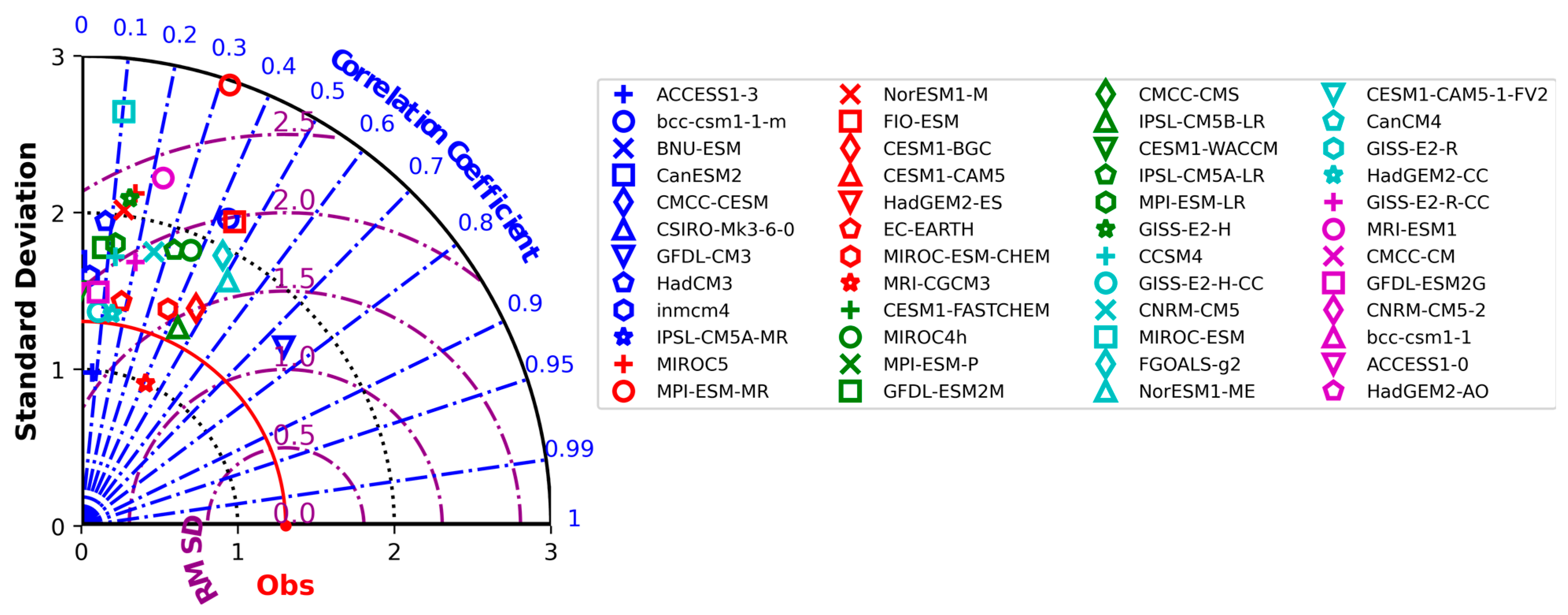
The establishment of the CNN is driven by the training dataset and validation dataset. Each dataset consists of input data (predictors) and labels data (predictand). Based on the historical simulations of NCDT during 1995–2004 (Figure 2), we selected six CMIP5 models (MPI-ESM-MR, MIROC5, GISS-E2-R-CC, FIO-ESM, CMCC-CMS, and ACCESS1-0) with relatively small deviations for training the CNN; the training period was 1852–1991. Note that most models showed relatively poor correlation coefficients, but we assumed that a few CMIP5 models would be able to capture the response of the tropical (or subtropical) SST forcing on East Asia [30,31,32,33]. The ERA5 reanalysis data (observation) during 1995–2017 were utilized as the validation dataset of the CNN. The ERA5 reanalysis data covers the period from 1950 to the present and has good evaluation applicability, especially in terms of the mean SLP and t2m [34]. Considering the high impacts of the SST and EAWM, which can be characterized by the Siberian-Mongolian high on NCDT, we selected monthly t2m and sea-level pressure (SLP) over the Northern Hemisphere (0°–360° E, 25° S–90° N) as predictors. Before inputting the predictors to CNN, it was necessary to preprocess the original data. In this process, because different datasets and different members of CMIP5 have inconsistent levels of resolution, the original predictors’ data were first gridded to a 5 × 5 grid, and then normalized by the standard deviation to unify different atmospheric elements to the same order of magnitude. Such processed data were eventually combined as input data. There is a four-year gap between the training dataset and validation dataset to prevent the atmospheric and oceanic memories in the training period from interfering with the validation period. There is no weighting among the six historical simulations of the CMIP5, and the total sample size of the training dataset is 840 (140 for each CMIP5 model). The models were trained with lead times of 1, 2, 3, …, and 12 months separately. For each month of lead time, we also trained the model for 4 times and obtained 4 ensemble members; the average of the output of the 4 ensemble members was calculated as prediction and for the final analysis.
In addition, to compare the CNN prediction skill, a typical traditional statistical model was set as a baseline: a Multiple Linear Regression model (MLR) was driven by the same training dataset. In the MLR, the dependent variable y can be calculated by the equation in which bi denotes the weight of each independent variable xi:
y = 1 n b i x i + b 0
where n denotes the number of independent variables and is calculated based on the longitude and latitude numbers of predictors. In this study, the MLR shared the same input and output used in the CNN. The value xi denotes the t2m and SLP standardized maps over 0°–360° and 25° S–90° N. The value y denotes the NCDT.
Finally, we compared the results of the CNN to the SEAS5 and the MLR model results. The forecast skill was computed as the correlation coefficient between the outputs of these models and the ERA5 Reanalysis.
To understand how the CNN can successfully predict NCDT for a specific lead time, we utilized a heat map [25] to analyze the CNN. The contributions of the predictors at each point to the predictand can be quantified by a heat map. The heat map value for the neuron of the output layer at grid point ( x ,   y ) (indicated as h x , y ) was calculated by the following equation:
h x , y = n = 1 N { tanh [ m = 1 M L ( W F , m , n x , y v L , m x , y ) + b F , n X L Y L ] W O , n } + b O X L Y L
where X L and Y L denote the dimensions of the feature map in the third convolutional layer. N (50 here) denotes the number of neurons in the fully connected layer, M L (50 here) denotes the number of feature maps in the last convolutional layer, W F , m , n x , y denotes the weight at the grid point ( x ,   y ) (used to link the mth feature map in the last convolutional layer L to the nth neuron in the fully connected layer F), v L , m x , y denotes the value of the m th feature map of the last convolutional layer L at grid point ( x ,   y ) , b F , n denotes the bias of the nth neuron in the fully connected layer F, W O , n denotes the weight (used to link the nth neuron in the fully connected layer F to the output layer O), and b O denotes the bias of the output layer O.
After the heat map analysis, a regression analysis was used to investigate whether the relationship between the NCDT and the predictors shown in the heat map was consistent with that in observations and to discuss the possible physical mechanism between the high-value area in the heat map and the NCDT. The regression equation can be calculated as:
y ˜ ( i ,     j ) = b 0 + b 1 x
where y ˜ ( i ,   j ) is the regressed value of y ( i , j ) onto x at grid ( i ,   j ) ; b 0 , b 1 can be calculated as follows, where m x ( m y ( i , j ) ) denotes the mean of the time series of x ( y ( i , j ) ), and n denotes the length of the time series.
{ b 1 = 1 n t = 1 n x t y t ,   ( i , j ) m x · m y ( i , j ) 1 n t = 1 n x t 2 m x 2 b 0 = m y ( i , j ) b 1 m x

2.2. Skill Metrics

The performances of the CNN, SEAS5, and MLR models were mainly evaluated by the Pearson correlation coefficient (CC), which can be calculated as follows:
CC ( y , y ˜ ) = i = 0 n ( y i m y ) ( y ˜ i m y ˜ ) i = 0 n ( y i m y ) 2 ( y ˜ i m y ˜ ) 2
where y ˜ i is the predicted value of ith sample and y i is the corresponding observation; n is the number of samples (the length of the time series); m y is the mean of the time series y , and m y ˜ is the mean of the time series y ˜ . Additionally, the root mean square error (RMSE), mean absolute error (MAE), and mean absolute percentage error (MAPE) are calculated as evaluation metrics:
RMSE ( y , y ˜ ) = 1 n i = 0 n 1 ( y i y ˜ i ) 2
MAE ( y , y ˜ ) = 1 n i = 0 n 1 | y i y ˜ i |
MAPE ( y , y ˜ ) = 1 n i = 0 n 1 | y i y ˜ i | max ( ε , | y i | )
where ε is an arbitrary, small, yet strictly positive number in order to avoid undefined results when y is zero.

2.3. Earth System Model

The third version of the Nanjing University of Information Science and Technology Earth System Model (NESM3.0) was used in this study [35,36,37]. The NESM3.0 includes atmosphere, ocean, sea ice, and land surface component models that are fully coupled by an explicit coupler. The atmosphere model has the resolution of T63L47. The resolution of the ocean model is 1°, with the meridional resolution refined to 1/3° over the equatorial region; the vertical resolution is 46 vertical layers, with the first 15 layers in the top 100 m. The NESM3.0 simulates not only reasonable climatology and East Asia winter monsoons, but also the key characteristics of decadal and multi-decadal variabilities [33,38,39,40]. Two experiments were conducted to examine the impact of the Northeast Pacific SST on North China winter temperature. The first model simulation was run using the observed SST anomalies (NESM_NEP), the second, using the climatological SST (NESM_CLIM) specified over the Northeast Pacific domain (170°–130° W, 10°–30° N) with a 1-day nudging timescale. For all the experiments, the model was integrated from 1950 to 2018 using external forces (greenhouse gases, solar constant, aerosol concentration, ozone, etc.) based on the sixth phase of the Coupled Model Intercomparison Project (CMIP6) protocols and data from the past 40 years (1979–2018). The initial conditions for integration were obtained from a historical run based on the CMIP6 protocols.

3. Results

3.1. Performance of CNN

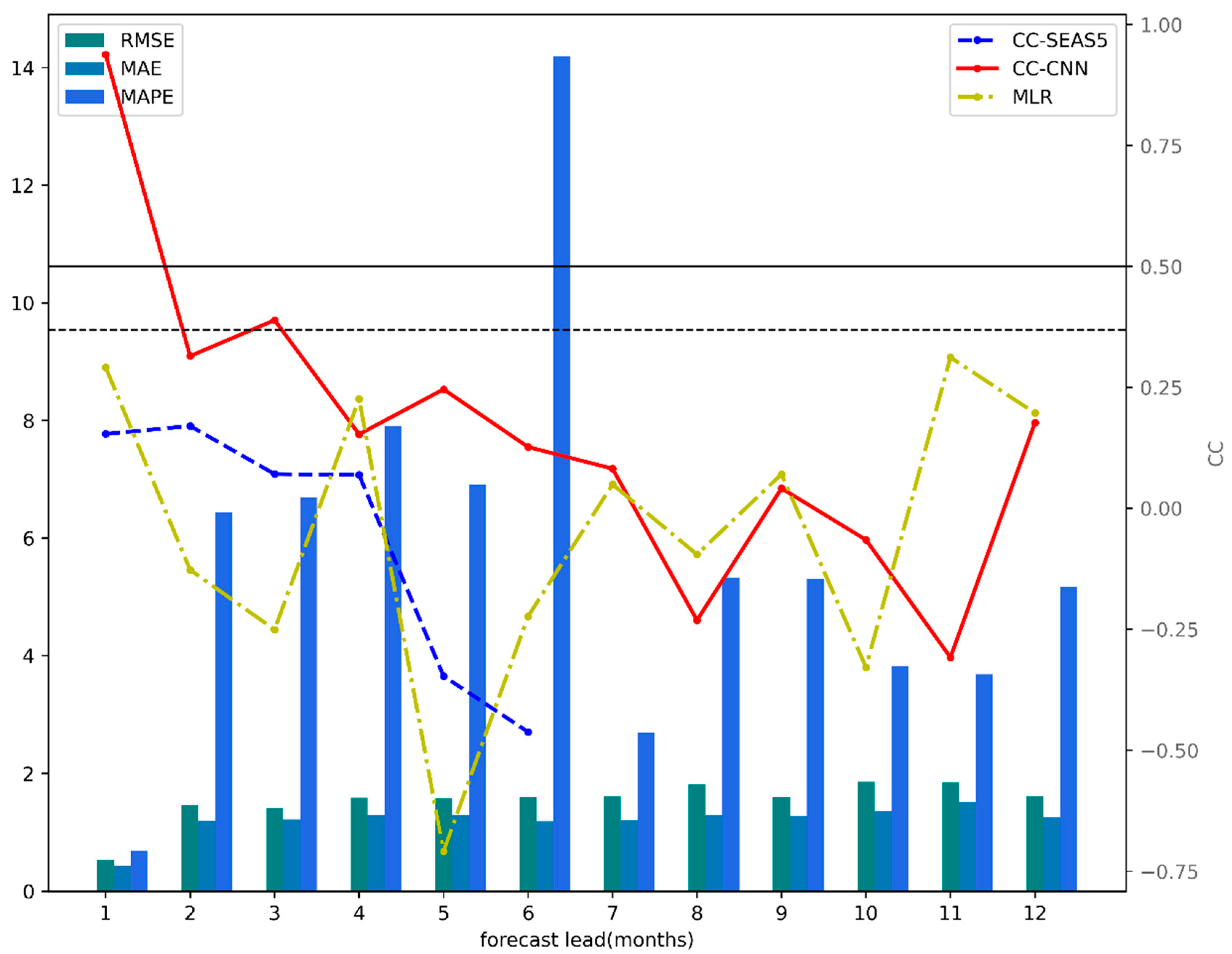
After training on a dataset based on CMIP5 historical simulations, the CNN showed improved prediction skill for the whole validation period (1995–2017) compared to that of the SEAS5 model (Figure 3). The SEAS5 is one of the best seasonal forecast systems in the world, providing forecasts within a 6-month lead time. The CNN showed a high level of prediction skill at a 1-month lead time with a correlation skill of 0.92 and maintained relatively high skill up to a 6-month lead time. The average prediction skill of CNN at 1–6 months was 0.33, outperforming the SEAS5 (−0.053).
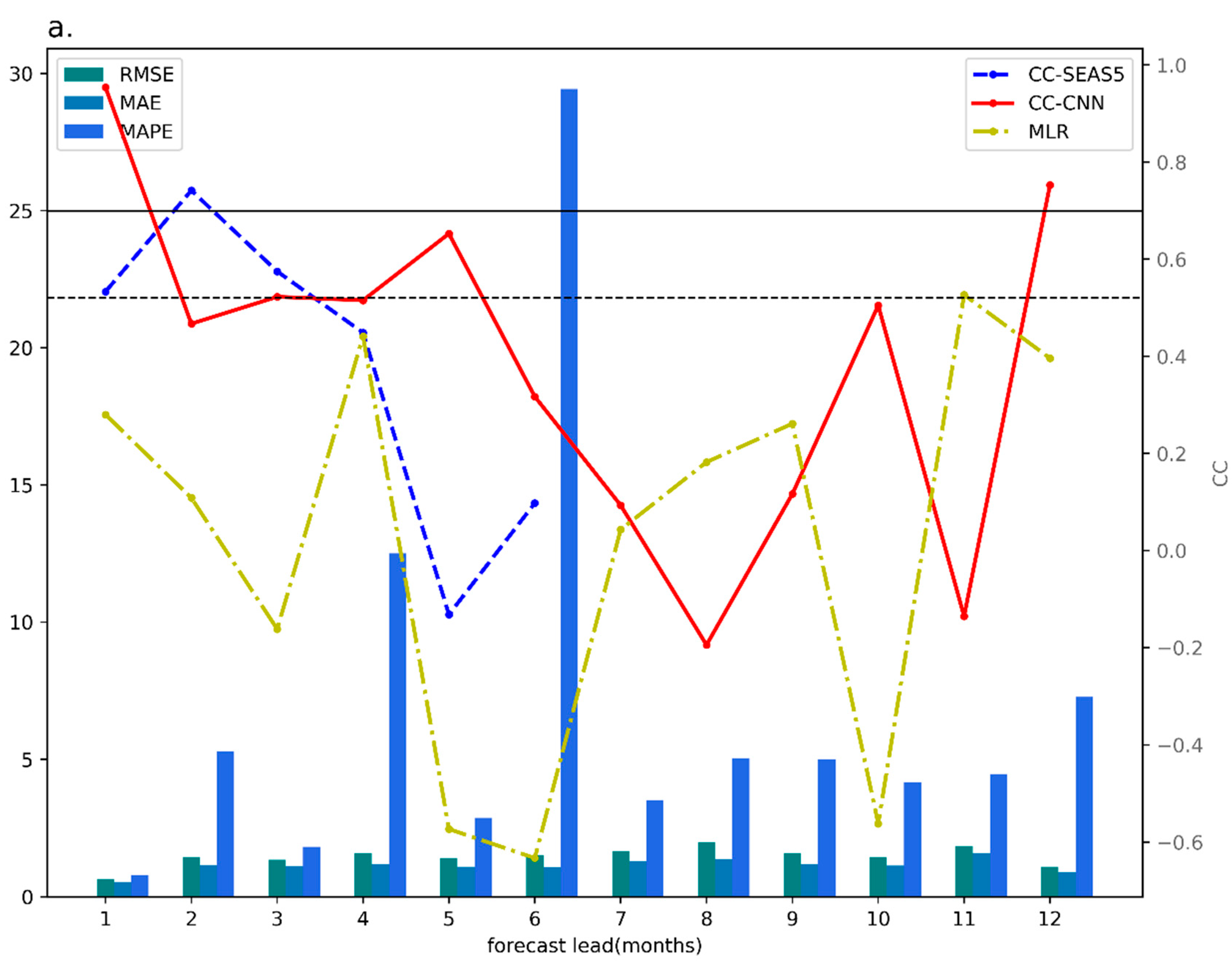
The CNN obtained its best performance level in the most recent 10 years (2008–2017, Figure 4a), showing high prediction skill at a 1-month lead time with a correlation skill of 0.95, and maintaining a relatively high level of prediction skill (except for a slight drop at the 2-month lead time) up to a lead time of 5 months. The prediction skill decreased from a 6-month lead time, and suddenly increased at a 10- or 12-month lead time. The high prediction skill at the 1-month lead time may be due to an autocorrelation between the November and December temperatures. The reason for the rapid increase in prediction skill at the 12-month lead time is not clear to us. We suspect that it may result from long-term climate variabilities (e.g., the ENSO, PDO, and AMO). In our comparison with SEAS5, we focused on the forecasting skills from 1- to 6-month lead times in this study. The prediction skill of the SEAS5 was relatively low (correlation skill of 0.53) for a 1-month lead time, with high correlation skills (up to 0.75) at the 2- and 3-month lead times. The prediction skill largely reduced to −0.13 at the 5-month lead time, implying no prediction skill after the 4-month lead time. The CNN has an advantage for a long lead time (>4 months) over the SEAS5. The average prediction skill at a 1–6-month lead time for the CNN was 0.57, outperforming the time of the SEAS5 (0.38). On the other hand, the MLR showed very low prediction skill for all lead times.
Notice that the sudden decrease in prediction skill of the SEAS5 and the difference in the prediction skill between the SEAS5 and the CNN reached its maximum at a 5-month lead time. Hence, we focused on the details of the results from a 5-month lead time.
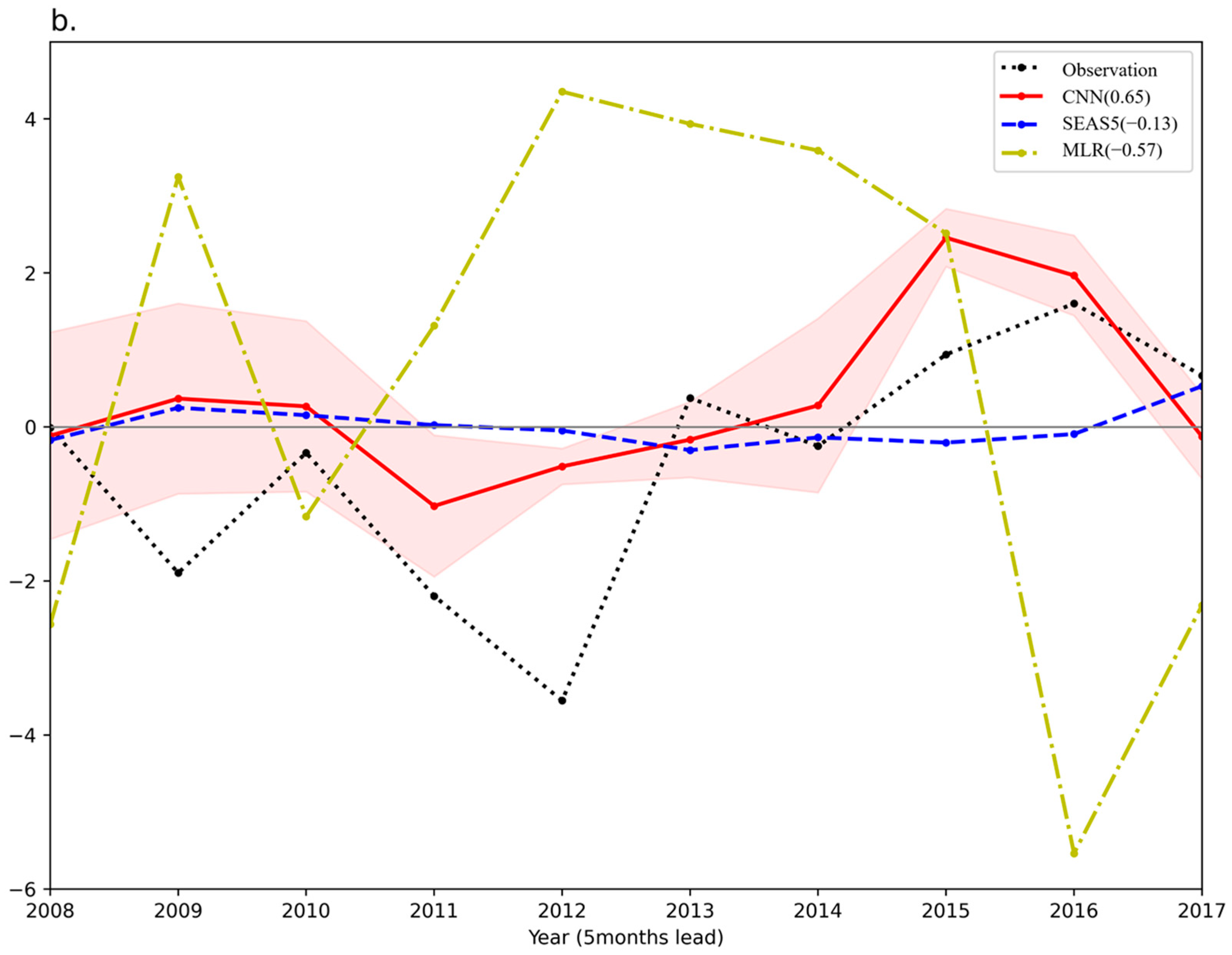
The NCDT index for the 5-month-lead forecast demonstrated that the CNN model reasonably predicted the NCDT amplitude (Figure 4b). The SEAS5 failed to capture the interannual variability of the NCDT, showing an inverse variation in contrast to the observation, and its magnitude was much smaller than the observed records. Additionally, a phase transition from relatively cold (2008–2013) to relatively warm (2013–2017) shown in observational NCDT was captured by the CNN. The MLR showed false amplitude for most years, and the amplitude of variance was relatively larger than the observation. The results show that the CNN model has the potential to make up for the weakness of the state-of-the-art dynamical models and traditional statistical models and to predict the NCDT with precision to some extent.

3.2. Possible Physical Interpretation

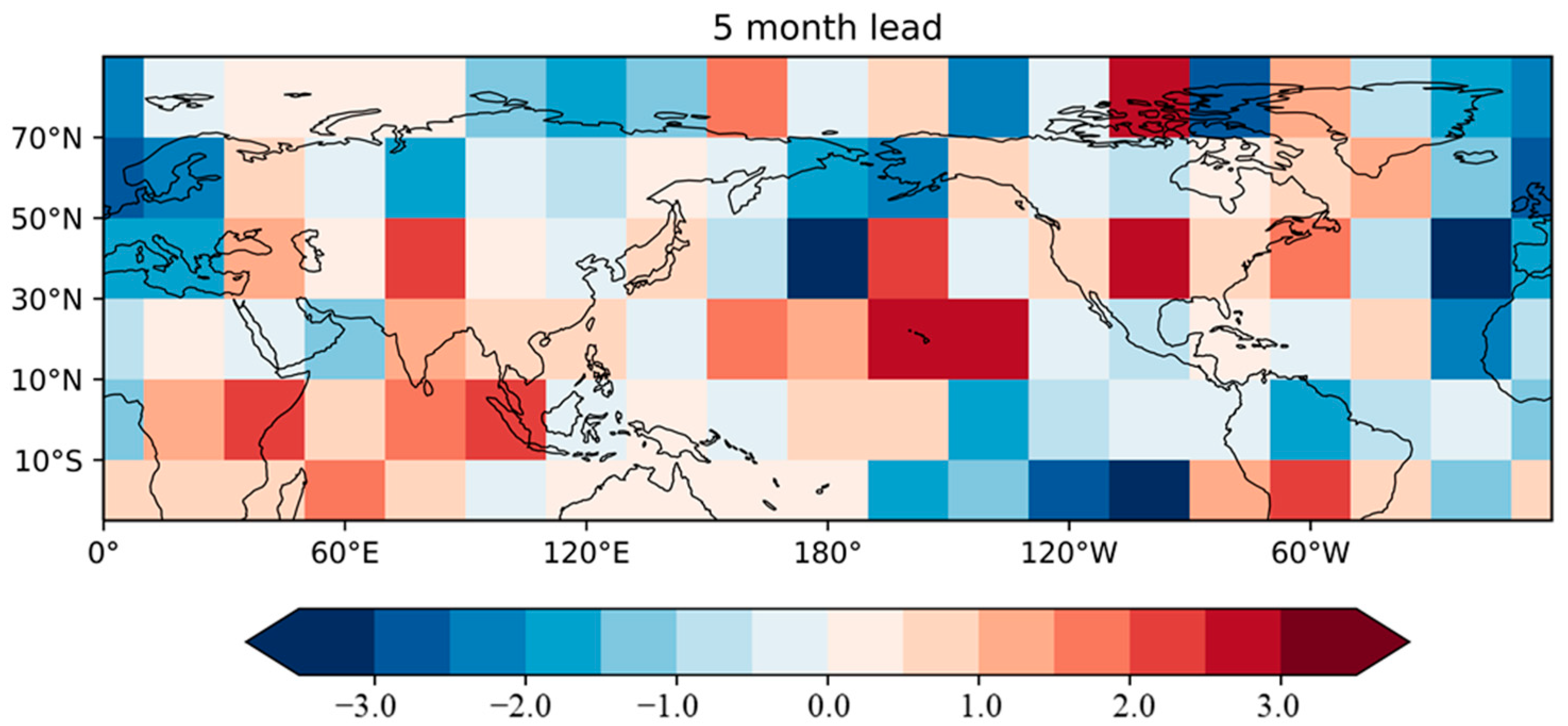
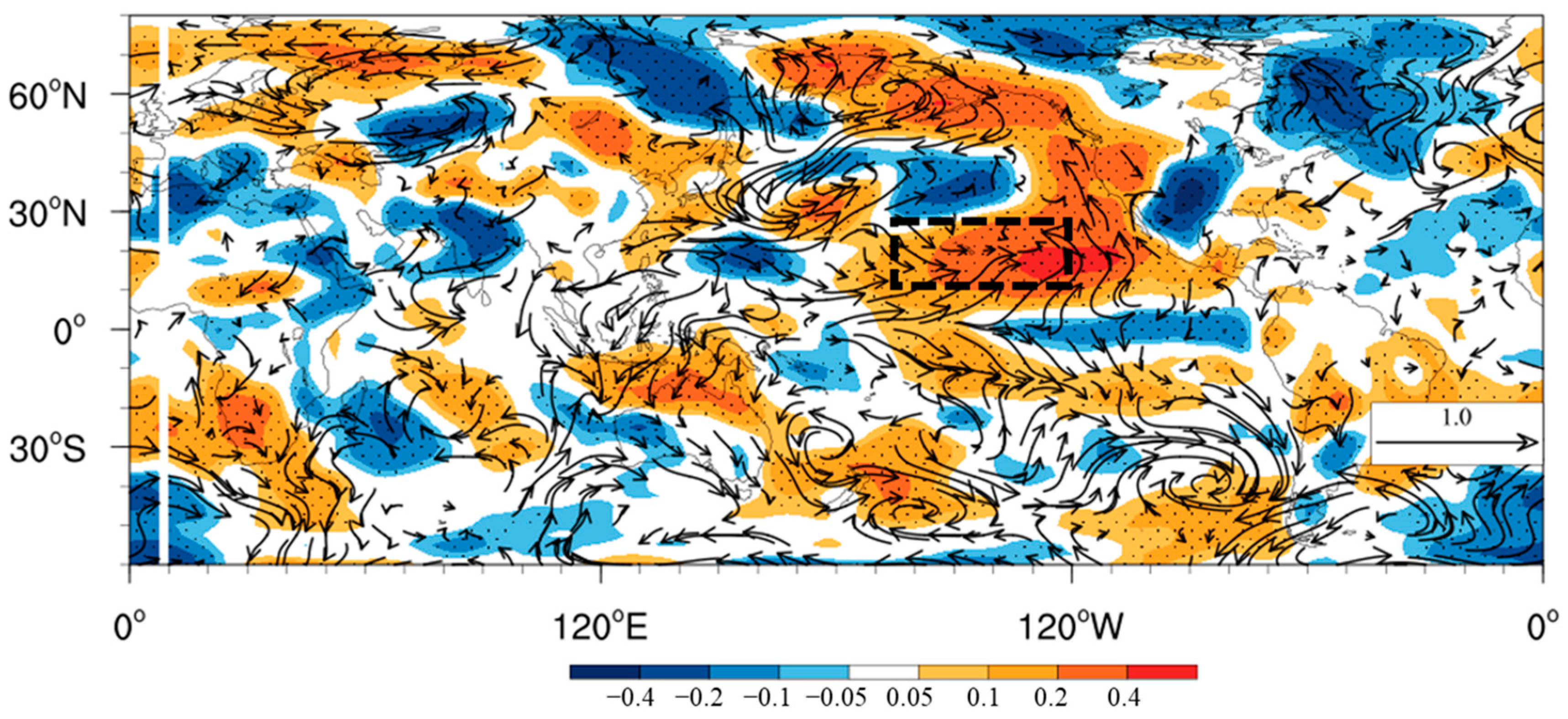
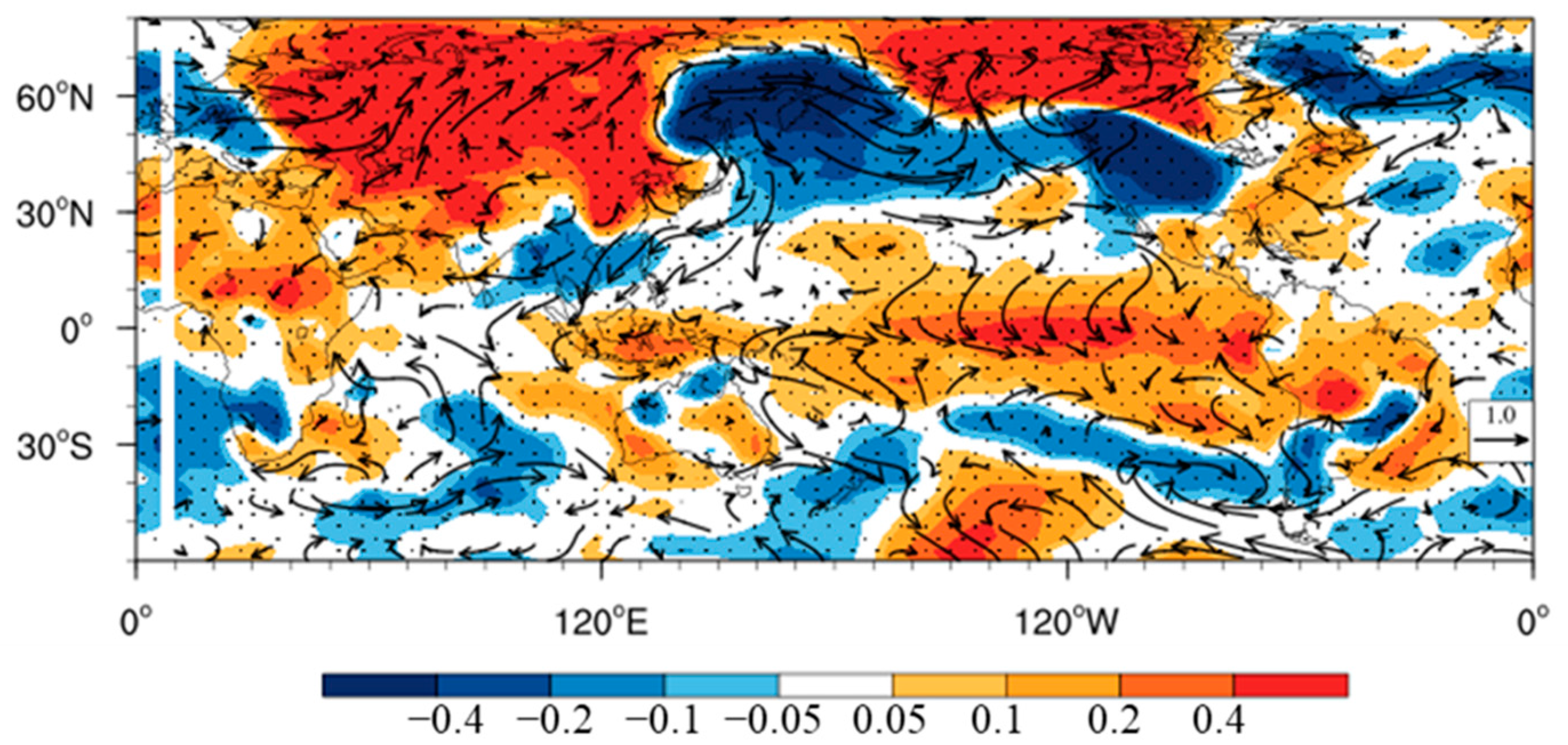
To understand how the CNN model could improve prediction skill for the NCDT with relatively long lead times, we conducted a heat map analysis for the 5-month-lead forecast during the validation periods (Figure 5). The heat map shows how much the predictors (SLP and t2m) at each grid point contributed to the NCDT; dark red (blue) over a specific region represents more positive (negative) contribution to the predictors. The heat map shows that the t2m or SLP anomalies over the subtropical Northeast Pacific, North Pacific, and eastern Beaufort Sea in July mainly contributed to the improved prediction of the NCDT. The SST signal over the Northeast Pacific (170°–130° W, 10°–30° N) highlighted by the CNN may be closely linked to the NCDT. We examined the relationship between the NCDT and July t2m and surface wind from the observations. Figure 6 shows the regressed July t2m onto the NCDT. The results show that the warming over North China in the winter season is related to the Northeast Pacific SST warming and to the cooling of the North Pacific and western America. Compared to the results of the heat map analysis, the Northeast Pacific warming in the boreal summer could be linked to the warming over North China in the boreal winter. We noted that it is difficult to find factors with long-term memory over the continental US. Thus, this topic will be discussed in a further study.
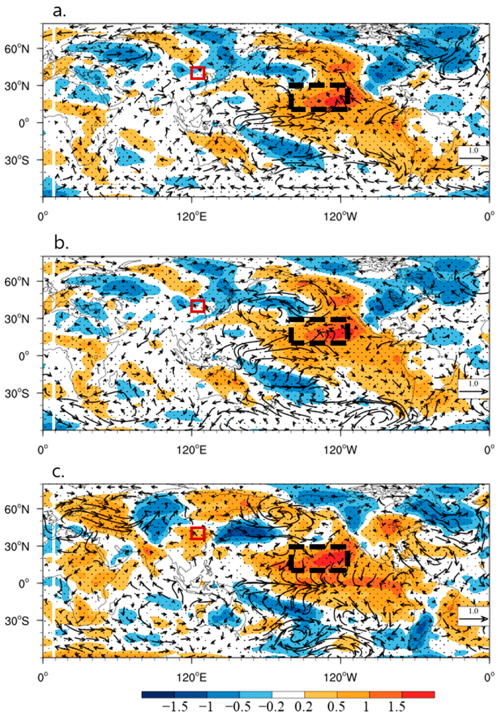
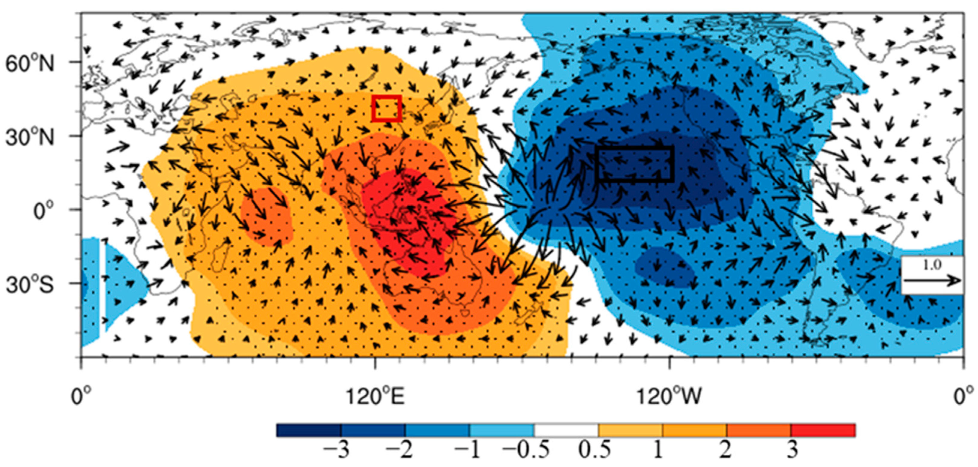
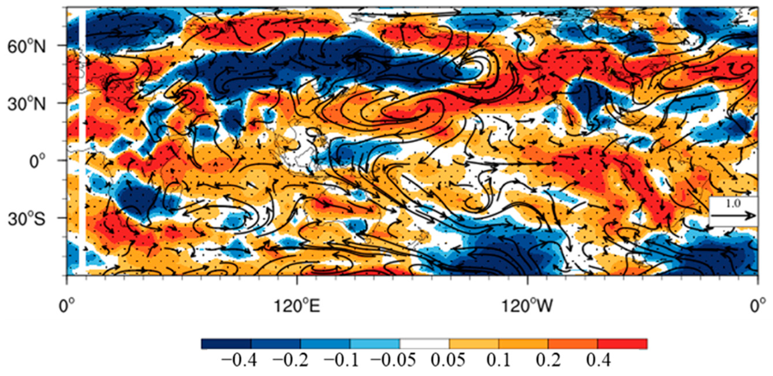
We explore how the Northeast Pacific SST in the boreal summer affects the t2m in December over the North China region using observed and reanalysis data next in Figure 7a, which shows the regressed July t2m and surface wind onto the July Northeast Pacific SST. There is a broad warming in the central astern Pacific. The warming in the North (South) Pacific extends to the Bering Sea (a region south of Chile). Corresponding westerly anomalies are seen in the western and central tropical Pacific, and cyclonic flows occur in the North Pacific. The poleward anomalies may further generate westerlies up to December over the western and central Pacific, inducing El Niño development (Figure 7c). The warming in the eastern Pacific generates an upward motion there and a sinking motion in the western Pacific (Figure 8). The sinking motion may induce anticyclonic flow and increase northward flow, generating warming in the East China Sea and North China (Figure 7c).
To investigate the relationship between the Northeast Pacific and the NCDT, we conduct two additional experiments: the NESM3.0 was integrated for 1950–2017 with the observed SST (NESM_NEP) or climatological SST (NESM_CLIM) over the Northeast Pacific. The simulation with the observed SST was able to capture the observed horizontal pattern (Figure 9); strong warming (cooling) occurs in the central and eastern tropical Pacific (North Pacific), and the corresponding westerlies in the equatorial Pacific and the cyclonic flows in the North Pacific are well simulated. The NESM3.0 simulation with climatological SST failed to reproduce the observed pattern (Figure 10). There is no warming over the Northeast Pacific; and strong warming does appear in the North Pacific, which is not seen in the observation. The equatorial westerlies are relatively weak; the corresponding El Niño signal is weak and shifted southeastward, inducing cooling (warming) in North (South) China. These results suggest that warming in the Northeast Pacific in the boreal summer could induce warming over North China in the boreal winter by developing an El Niño event.

4. Summary and Conclusions

In this study, we developed a CNN (Convolutional Neural Network)-based DL (Deep Learning) model for the seasonal forecast of the NCDT (North China December t2m). We used t2m and SLP (sea-level pressure) as predictors; the model was trained by six CMIP5 (the fifth phase of the Coupled Model Intercomparison Project) historical simulations. Forecasts of SEAS5 (ECMWF’s fifth generation seasonal forecast system) and MLR (Multi Linear Regression model) were utilized for comparison with the CNN. The CNN produces significantly improved prediction skill over the SEA5 and MLR, particularly in the range of a 5-month to 12-month lead time. In addition, the forecast of the CNN with the 5-month lead time depicted the fluctuations of the NCDT during the La Niña event in 2011 and the El Niño event in 2015. The Northeast Pacific SST anomalies in July were shown by a heat map analysis to make a strong contribution to the NCDT anomalies; further analysis supported this result. In July, warming in the Northeast Pacific may be favorable to an El Niño event in the coming winter by generating westerlies in the western and central Pacific. The warming by El Niño generates sinking (rising) motion over the western Pacific (eastern Pacific) and induces anticyclonic flows and northward transport in the Northwest Pacific, inducing warming in the North China region. The skill of the CNN with a 5-month lead time can be explained by such a reasonable mechanism, implying DL is a reliable tool in North China winter temperature seasonal forecast.
Though the results shown here are promising, the following points need further study. Only two predictors were selected here; it is necessary to input more different atmospheric and oceanic elements from different levels to the CNN, which may result in different results. Heat map analysis suggested a significant contribution from the North Pacific and Beaufort Sea; these regions may be linked to the NCDT, a claim which needs to be analyzed in further studies. The prediction skill of the CNN model depends on the validation period. When we increased the validation period from 1995 to 2017, though it still outperformed the SEAS5, the CNN skill score decreased (Figure 3), which may be attributed to a different background mean state. The decadal or multi-decadal variability can induce a different background climate, which may affect the model’s prediction skill. Original data from CMIP5 historical simulations were used to train the CNN; however, the quality of the CMIP5 data is quite low. Correcting the bias of the CMIP5 data may be a way to consider for bettering the performance of the DL model, and the DL has been proved to be a powerful tool for correcting the bias of numerical weather prediction models [41]. These issues will be discussed in our further study.

Author Contributions

Y.-M.Y. designed the model’s overall structure and the strategy; L.G. and Y.-M.Y. developed the model and analyzed the result; Y.-G.H. and J.-H.K. provided source code; Y.-M.Y. and L.G. drafted the original paper and Q.L. contributed to revising the paper. All authors have read and agreed to the published version of the manuscript.

Funding

This research was funded by the National Natural Science Foundation of China, grant number 42088101.

Data Availability Statement

Please contact Young-Min Yang ([email protected]) to obtain the source code and data for all model experiments.

Acknowledgments

We acknowledge the World Climate Research Programme’s Working Group on Coupled Modelling for their CMIP5 data. We acknowledge the ERA5 reanalysis and SEAS5 from Copernicus Climate Change Service (C3S). We thank two anonymous reviewers for providing constructive comments that helped us to improve our manuscript.

Conflicts of Interest

The authors declare no conflict of interest.

References

  1. China Meteorological Administration. China Climate Bulletin; China Meteorological Press: Beijing, China, 2013.
  2. Miao, Q.; Gong, Y.F.; Deng, R.J.; Wei, N. Impacts of the low-frequency oscillation over the extra-tropics of the Northern Hemisphere on the extreme low temperature event in Northeast China in the winter of 2012/2013. Chin. J. Atmos. Sci. 2016, 40, 817–830. (In Chinese) [Google Scholar]
  3. Zheng, F.; Yuan, Y.; Ding, Y.; Li, K.; Fang, X.; Zhao, Y.; Sun, Y.; Zhu, J.; Ke, Z.; Wang, J.; et al. The 2020/21 Extremely Cold Winter in China Influenced by the Synergistic Effect of La Niña and Warm Arctic. Adv. Atmos. Sci. 2021, 39, 546–552. [Google Scholar] [CrossRef]
  4. Wang, J.; Tang, K.; Feng, K.; Lin, X.; Lv, W.; Chen, K.; Wang, F. High Temperature and High Humidity Reduce the Transmission of COVID-19. SSRN Electron. J. 2020, 11, e043863. [Google Scholar] [CrossRef] [Green Version]
  5. Clark, R.T.; Bett, P.E.; Thornton, H.E.; Scaife, A.A. Skillful Seasonal Predictions for the European Energy Industry. Environ. Res. Lett. 2017, 12, 024002. [Google Scholar] [CrossRef]
  6. Wang, H.; Fan, K.; Sun, J.; Li, S.; Lin, Z.; Zhou, G.; Chen, L.; Lang, X.; Li, F.; Zhu, Y.; et al. A review of seasonal climate prediction research in China. Adv. Atmos. Sci. 2015, 32, 149–168. [Google Scholar] [CrossRef]
  7. Rasmusson, E.M.; Carpenter, T.H. Variations in Tropical Sea Surface Temperature and Surface Wind Fields Associated with the Southern Oscillation/El Niño. Mon. Weather Rev. 1981, 110, 148–162. [Google Scholar] [CrossRef]
  8. Yan, H.M.; Xiao, Z.N. The Numerical Simulation of the Indian Ocean SSTA Influence on Climatic Variations over Asian Monsoon Region. J. Trop. Meteor. 2000, 16, 18–27. (In Chinese) [Google Scholar]
  9. Chen, P.Y.; Ni, Y.Q.; Yin, Y.H. Diagnostic Study on the Impact of the Global Sea Surface Temperature Anomalies on the Winter Temperature Anomalies in Eastern China in Past 50 Years. J. Trop. Meteor. 2001, 17, 371–380. (In Chinese) [Google Scholar]
  10. Zhao, F.M.; Zhu, X.J.; Li, F.; Wang, Z.Q.; Gu, J.Y.; Wang, M.L. Relationship between SSTA in Japan Current Region and Temperature and Precipitation in China Winter. Meteor. Environ. Sci. 2007, 30, 28–31. (In Chinese) [Google Scholar]
  11. Zhu, Y.M.; Yang, X.Q. Relationships between Pacific Decadal Oscillation (PDO) and Climate Variabilities in China. Acta Meteor. Sin. 2003, 61, 641–654. (In Chinese) [Google Scholar]
  12. Li, S.L.; Wang, Y.M.; Gao, Y.Q. A review of the Researches on the Atlantic Multidecadal Oscillation (AMO) and Its Climate Influence. Trans. Atmos. Sci. 2009, 32, 458–465. (In Chinese) [Google Scholar]
  13. Wang, B.; Wu, Z.; Chang, C.-P.; Liu, J.; Li, J.; Zhou, T. Another Look at Interannual-to-Interdecadal Variations of the East Asian Winter Monsoon: The Northern and Southern Temperature Modes. J. Clim. 2010, 23, 1495–1512. [Google Scholar] [CrossRef] [Green Version]
  14. Lee, J.-Y.; Lee, S.-S.; Wang, B.; Ha, K.-J.; Jhun, J.-G. Seasonal prediction and predictability of the Asian winter temperature variability. Clim. Dyn. 2013, 41, 573–587. [Google Scholar] [CrossRef] [Green Version]
  15. Huang, F.; Gao, C.H. Interannual Variations of Winter Temperature in East Asia and Their Relationship with Sea Surface Temperature and Sea Ice Concentration. Period. Ocean Univ. China 2012, 42, 7–14. [Google Scholar]
  16. Chen, X.L.; Wu, H.B.; Ding, G.L.; He, X.X. Ensemble Canonical Correlation Prediction Method of Winter Temperature over China. J. Nanjing Inst. Meteorol. 2007, 30, 623–631. [Google Scholar]
  17. Johnson, S.J.; Stockdale, T.N.; Ferranti, L.; Balmaseda, M.A.; Molteni, F.; Magnusson, L.; Tietsche, S.; Decremer, D.; Weisheimer, A.; Balsamo, G.; et al. SEAS5: The new ECMWF seasonal forecast system. Geosci. Model Dev. 2019, 12, 1087–1117. [Google Scholar] [CrossRef] [Green Version]
  18. Baldi, P.; Sadowski, P.; Whiteson, D. Searching for exotic particles in high-energy physics with deep learning. Nat. Commun. 2014, 5, 4308. [Google Scholar] [CrossRef] [Green Version]
  19. Alipanahi, B.; Delong, A.; Weirauch, M.T.; Frey, B.J. Predicting the sequence specificities of DNA- and RNA-binding proteins by deep learning. Nat. Biotechnol. 2015, 33, 831–838. [Google Scholar] [CrossRef]
  20. Schütt, K.; Arbabzadah, F.; Chmiela, S.; Müller, K.R.; Tkatchenko, A. Quantum-chemical insights from deep tensor neural networks. Nat. Commun. 2017, 8, 6–13. [Google Scholar] [CrossRef] [Green Version]
  21. Reichstein, M.; Camps-Valls, G.; Stevens, B.; Jung, M.; Denzler, J.; Carvalhais, N. Deep learning and process understanding for data-driven Earth system science. Nature 2017, 566, 195–204. [Google Scholar] [CrossRef] [PubMed]
  22. Liu, Y.; Racah, E.; Correa, J.; Khosrowshahi, A.; Lavers, D.; Kunkel, K.; Collins, W. Application of deep convolutional neural networks for detecting extreme weather in climate datasets. arXiv 2016, arXiv:1605.01156. [Google Scholar]
  23. Racah, E.; Beckham, C.; Maharaj, T.; Ebrahimi Kahou, S.; Prabhat, M.; Pal, C. Extreme Weather: A large-scale climate dataset for semi-supervised detection, localization, and understanding of extreme weather events. Adv. Neural Inf. Process. Syst. 2017, 30, 3405–3416. [Google Scholar]
  24. Weyn, J.A.; Durran, D.R.; Caruana, R. Can Machines Learn to Predict Weather? Using Deep Learning to Predict Gridded 500-hPa Geopotential Height from Historical Weather Data. J. Adv. Model. 2019, 11, 2680–2693. [Google Scholar] [CrossRef]
  25. Ham, Y.G.; Kim, J.H.; Luo, J.J. Deep learning for multi-year ENSO forecasts. Nature 2019, 573, 568–572. [Google Scholar] [CrossRef]
  26. Choe, Y.J.; Yom, J.H. Improving accuracy of land surface temperature prediction model based on deep-learning. Spat. Inf. Res. 2020, 28, 377–382. [Google Scholar] [CrossRef]
  27. Jia, H.; Yang, D.; Deng, W.; Wei, Q.; Jiang, W. Predicting land surface temperature with geographically weighed regression and deep learning. Wiley Interdiscip. Rev. Data Min. Knowl. Discov. 2021, 11, e1396. [Google Scholar] [CrossRef]
  28. Lecun, Y.; Bengio, Y.; Hinton, G. Deep learning. Nature 2015, 521, 436–444. [Google Scholar] [CrossRef] [PubMed]
  29. Taylor, K.E.; Stouffer, R.J.; Meehl, G.A. An Overview of CMIP5 and the Experiment Design. Bull. Am. Meteorol. Soc. 2012, 93, 485–498. [Google Scholar] [CrossRef] [Green Version]
  30. Wei, K.; Xu, T.; Du, Z.; Gong, H.; Xie, B. How well do the current state-of-the-art CMIP5 models characterise the climatology of the East Asian winter monsoon? Clim. Dyn. 2014, 43, 1241–1255. [Google Scholar] [CrossRef]
  31. Wu, B.; Zhou, T. Relationships between ENSO and theEast Asian–western North Pacific monsoon: Observations versus 18 CMIP5 models. Clim. Dyn. 2016, 46, 729–743. [Google Scholar] [CrossRef]
  32. Yang, Y.M.; Wang, B.; Li, J. Improving seasonal prediction of east Asian summer rainfall using NESM3.0: Preliminary results. Atmosphere 2018, 9, 487. [Google Scholar] [CrossRef] [Green Version]
  33. Li, J.; Wang, B.; Yang, Y.M. Diagnostic metrics for evaluating model simulations of the East Asian monsoon. J. Clim. 2020, 33, 1777–1801. [Google Scholar] [CrossRef]
  34. Meng, X.G.; Guo, J.J.; Han, Y.Q. Preliminary assessment of ERA5 reanalysis data. J. Mar. Meteorol. 2018, 38, 91–99. [Google Scholar]
  35. Yang, Y.M.; Wang, B. Improving MJO simulation by enhancing the interaction between boundary layer convergence and lower tropospheric heating. Clim. Dyn. 2019, 52, 4671–4693. [Google Scholar] [CrossRef]
  36. Yang, Y.-M.; Wang, B.; Cao, J.; Ma, L.; Li, J. Improved historical simulation by enhancing moist physical parameterizations in the climate system model NESM3.0. Clim. Dyn. 2020, 54, 3819–3840. [Google Scholar] [CrossRef]
  37. Yang, Y.-M.; Cho, J.-A.; Moon, J.-Y.; Kim, K.-Y.; Wang, B. Improved boreal summer intraseasonal oscillation simulations over the Indian Ocean by modifying moist parameterizations in climate models. Clim. Dyn. 2021, 57, 2523–2541. [Google Scholar] [CrossRef]
  38. Yang, Y.M.; An, S.I.; Wang, B.; Park, J.H. A global-scale multidecadal variability driven by Atlantic multidecadal oscillation. Natl. Sci. Rev. 2020, 7, 1190–1197. [Google Scholar] [CrossRef] [Green Version]
  39. Yang, Y.M.; Lee, J.Y.; Wang, B. Dominant process for northward propagation of boreal summer intraseasonal oscillation over the Western North Pacific. Geophys. Res. Lett. 2020, 47, e2020GL089808. [Google Scholar] [CrossRef]
  40. Yang, Y.-M.; Park, J.-H.; An, S.-I.; Wang, B.; Luo, X. Mean sea surface temperature changes influence ENSO-related precipitation changes in the mid-latitudes. Nat. Commun. 2021, 12, 1495. [Google Scholar] [CrossRef]
  41. Han, L.; Chen, M.; Chen, K.; Chen, H.; Zhang, Y.; Lu, B.; Qin, R. A deep learning method for bias correction of ECMWF 24–240 h forecasts. Adv. Atmos. Sci. 2021, 38, 1444–1459. [Google Scholar] [CrossRef]
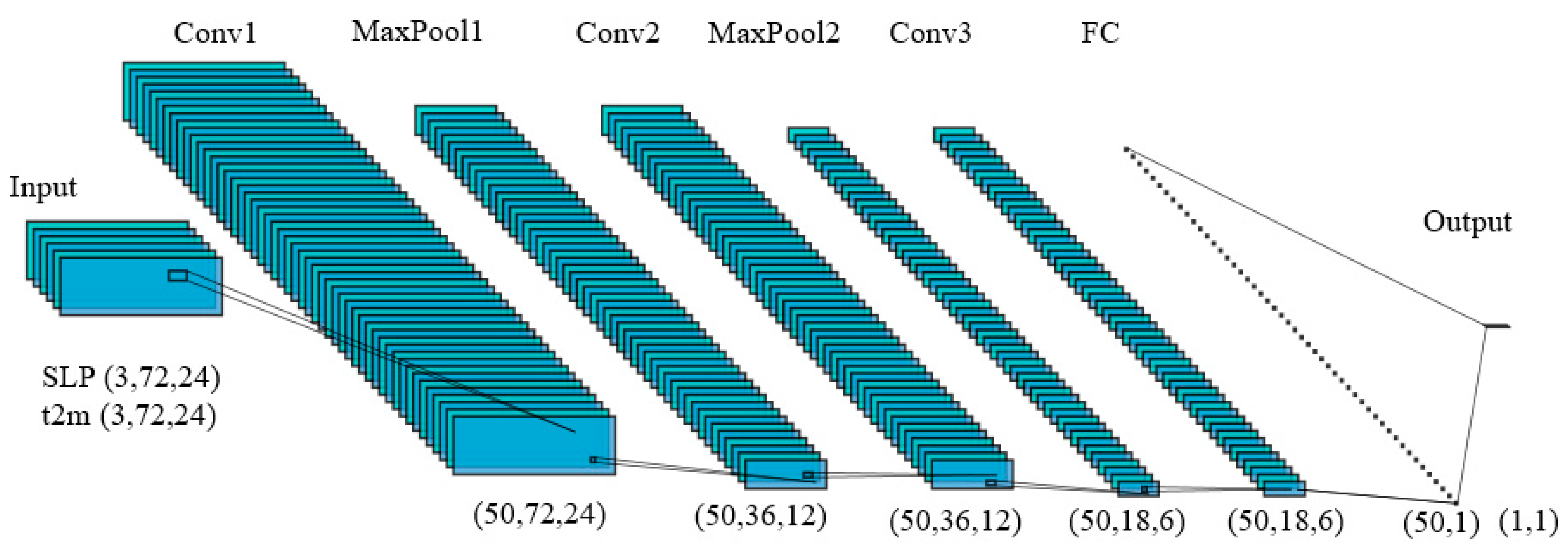
Figure 1. Schematic of the CNN used in this study. The CNN contained one input layer (predictor), three convolution layers (Conv1, Conv2, and Conv3), two max-pooling layers (MaxPool1 and MaxPool2), one fully connected layer (FC), and one output layer (NCDT). The number of filters in convolution and hidden layers was set as 50. The variables of the input layer corresponded to the t2m and SLP (sea-level pressure) standardized maps (0°–360° E and 25° S–90° N).
Atmosphere 13 00702 g001
Figure 2. Taylor diagrams of December t2m anomalies for the CMIP5 models as compared to the observations (red dot, obtained from ERA5 reanalysis) over the North China region (110°–120° E, 35°–45° N). Ten years (1995–2004) of data were used for the analysis.
Atmosphere 13 00702 g002
Figure 3. Correlation skills of the predicted NCDT from CNN (red solid line), SEAS5 (blue dotted line), and MLR (yellow dash-dotted line); RMSE (teal bar), MAE (dark blue bar), and MAPE (sapphire-blue bar) between the predicted NCDT from CNN and observation during 1995–2017. The correlation skills above the black solid (dotted) line are significant at the level of 0.01 (0.05).
Atmosphere 13 00702 g003
Figure 4. (a) Same as Figure 3, but for 2008–2017. (b) Time series of observed NCDT (black dotted line) and its 5-month-lead prediction of CNN (red solid line; ensemble distributions are shaded by red), SEAS5 (blue solid line), and MLR (yellow dash-dotted line). Correlation skills are indicated in parentheses.
Atmosphere 13 00702 g004aAtmosphere 13 00702 g004b
Figure 5. The heat map of the CNN from the 5-month lead time. Positive (negative) values represent how predictors contribute to the prediction of a positive (negative) NCDT.
Atmosphere 13 00702 g005
Figure 6. Regressed July t2m (shading; K) and surface wind (vector; m s−1) anomalies onto NCDT from the observations. The black dotted box denotes the location of the Northeast Pacific. Stippling indicates significance at the 95% level from Student’s t-test. Black vectors are significant regressed surface wind anomalies at the 90% level from Student’s t -test.
Atmosphere 13 00702 g006
Figure 7. Regressed global t2m anomalies (shading; K) and surface wind anomalies (vector; m s−1) in (a) July, (b) September, and (c) December onto Northeast Pacific SST anomalies in July from the observation. Stippling indicates significant regressed SST anomalies at the 95% level from Student’s t -test. Black vectors are significant regressed surface wind anomalies at the 90% level from Student’s t -test. The black dotted (red solid) box denotes the Northeast Pacific (North China).
Atmosphere 13 00702 g007
Figure 8. Regressed DJF global 200-hPa velocity potential (shading; m2 s−1) and divergent flow (vector; m s−1) onto Northeast Pacific SST anomalies in July from the observation. Stippling indicates significant regressed velocity potential anomalies at the 95% level from Student’s t-test. Black vectors are significantly regressed 200-hPa divergent wind anomalies at the 95% level from Student’s t-test.
Atmosphere 13 00702 g008
Figure 9. Regressed global t2m anomalies (shading; K) and surface wind anomalies (vector; m s−1) in December onto Northeast Pacific SST anomalies in July from NESM3.0 with observed SST in the Northeast Pacific. Stippling indicates significant regressed SST anomalies at the 95% level from Student’s t-test. Black vectors are significant regressed surface wind anomalies at the 95% level from Student’s t-test.
Atmosphere 13 00702 g009
Figure 10. Same as Figure 8, but from NESM3.0 with climatological SST in the Northeast Pacific.
Atmosphere 13 00702 g010
Publisher’s Note: MDPI stays neutral with regard to jurisdictional claims in published maps and institutional affiliations.