Abstract
The ambient formation of secondary particulate matter (ambient FSPM) is commonly recognized as the major cause of severe PM2.5 air pollution in China. We present observational evidence showing that the ambient FSPM was too weak to yield a detectable contribution to extreme PM2.5 pollution events that swept northern China between 11 and 14 January 2019. Although the Community Multiscale Air Quality (CMAQ) model (v5.2) reasonably reproduced the observations in January 2019, it largely underestimated the concentrations of the PM2.5 during the episode. We propose a novel mechanism, called the “in-fresh-stack-plume non-precipitation-cloud processing of aerosols” followed by the evaporation of semi-volatile components from the aerosols, to generate PM2.5 at extremely high concentrations because of highly concentrated gaseous precursors and large amounts of water droplets in fresh cooling combustion plumes under poor dispersion conditions, low ambient temperature, and high relative humidity. The recorded non-precipitation-cloud processing of the aerosols in fresh stack combustion plumes normally lasts 20–30 s, but it prolongs as long as 2–5 min under cold, humid, and stagnant meteorological conditions and expectedly causes severe PM2.5 pollution events. Regardless of the presence of the natural cloud in the planetary boundary layer during the extreme events, the fast conversion of air pollutants in water droplets and the generation of the PM2.5 through the non-precipitation-cloud processing of aerosols always occur in fresh combustion plumes. The processing of aerosols is detectable using a nano-scan particle sizer assembled on an unmanned aerial vehicle to monitor the particle formation in stack plumes. In-fresh-stack-plume processed aerosols under varying meteorological conditions need to be studied urgently.
1. Introduction
As a result of great efforts to reduce air pollutant emissions in China, a large drop in the mass concentration of atmospheric particles with diameters smaller than 2.5 µm (PM2.5) has been reported in inland and coastal atmospheres in comparison with the observations since 2013 [1,2,3,4,5,6,7,8,9,10,11,12,13]. For instance, the reported annual average mass concentration of the PM2.5 in Beijing was 42 µg m−3 in 2019 and it decreased by approximately 50% relative to the value in 2013 (http://www.xinhuanet.com/politics/2020-01/03/c_1125419813.htm, accessed on 23 March 2022). However, severe PM2.5 air pollution events, with 24 h averages of mass concentration exceeding 200 µg m−3, still occur in northern China, including Beijing [10,14,15]. Surprisingly, severe PM2.5 pollution events continued to occur amid the peak period of the COVID-19 outbreak in 2020 [16,17]. Many hypotheses on the formation of secondary particulate matter (FSPM) in ambient air—referred to as “ambient FSPM” in this paper—have been suggested to interpret the severe events over the past decade [1,3,5,6,7,16,17,18,19,20,21,22]. The ambient FSPM is physically detectable in clean or slightly polluted atmospheres [23,24,25,26]. However, whether the mechanisms can yield a significant contribution to severe PM2.5 pollution events is controversial [1,13,16,17,18,19,20,21,22].
In addition to the ambient FSPM, the primary particulate matter emitted from stack combustion sources has also been recognized as an important contributor to the ambient PM2.5 [2,3,4,27,28,29,30,31]. To explore the contribution of the ambient FSPM to severe PM2.5 air pollution, we introduce a metric, that is, PM2.5/CO. CO is chemically stable in ambient air at the ground level and is an ideal indictor of the accumulation extent [3,29], although CO may not be necessarily derived from the same sources of PM2.5. A combination of the mass concentrations of the PM2.5 and the ratios of the PM2.5/CO allowed us to reasonably identify the contribution of accumulating and/or mixing the primary particulate matter to largely increase the PM2.5 [29] and then examining whether the contribution of the ambient FSPM to a largely increased PM2.5 is negligible or not. In addition, we highlight three technical terms, that is, (1) ambient FSPM, (2) primary particulate matter which has been generated prior to being released to ambient air, and (3) FSPM in fresh stack combustion plumes, which we refer to as the “in-fresh-stack-plume non-precipitation-cloud processing of aerosols” that lasts for dozens of seconds to several minutes with the rapid cooling of water vapor in seconds, the fast chemical conversion of chemicals in droplets, and the evaporation of water droplets to generate the PM2.5 afterward (see Figure 1a–d, Supplementary Materials Videos S1–5, and Feng et al. [27]). The FSPM in the fresh stack combustion plumes cannot be treated as the primary particulate matter while it is also largely different from the ambient FSPM. Although several studies in the literature reported the formation and dispersion of primary and secondary pollutants [32,33,34,35], the rapid cooling of water vapor and in-fresh-stack-plume non-precipitation-cloud processing of aerosols have never been considered. Figure 2a–h show how the PM2.5 and PM2.5/CO change under two contrasting conditions, that is, accumulation and dilution, in the presence or absence of the two formation mechanisms. The details are provided in Materials and Methods.

Figure 1.
(a) Schematic of in-fresh-stack-plume non-precipitation-cloud processing of aerosols; (b) contour plot of particle number concentration scanned by a nano-scan particle sizer mounted on an unmanned aerial vehicle flying through fresh combustion plumes (2) and ambient air (1, 3); (c,d) photos taken for the measurements.
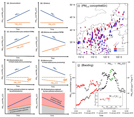
Figure 2.
Theoretical analysis of PM2.5 and PM2.5/CO change under two conditions, that is, accumulation and dilution, in the presence or absence of ambient FSPM and in-fresh-stack-plume non-precipitation-cloud processing of aerosols (a–h); red shadow and grey shadow represent the presence of ambient FSPM and that of evaporation of semi-volatile species, respectively, in (g,h); geographical distribution of 24 h average mass concentrations of PM2.5 over northern China on 12 (red bars) and 13 (blue bars) January 2019 (i); time series of hourly average mass concentrations of PM2.5 and PM2.5/CO ratios in µg m−3/mg m−3 (j) and their correlation on 9–13 January 2019 in Baoding; three colors of full markers in (j) represent different time data with almost invariant PM2.5/CO, and empty markers represent the remaining data.
With the above-mentioned technical terms in mind, an extreme PM2.5 pollution event that occurred on 11–14 January 2019 in the inland and coastal atmospheres across northern China provides an ideal example to explore the cause of severe PM2.5 pollution events in present-day China. In addition, the measurements and simulations during other periods were also used to facilitate the analysis.
2. Materials and Methods
2.1. Data Sources
The hourly average mass concentrations of air pollutants were obtained from air quality monitoring networks in China, where thousands of air quality monitoring sites have been established in hundreds of cities. The data for each day can also be downloaded from https://www.iqair.com/china, accessed on 23 March 2022; however, the web-based raw data have no quality control and need to be processed before analysis. Note that the hourly average of each air pollutant in Baoding reflects the mean value of its concentrations at tens of local stations; the same is true in the case of Langfang (Figure S1). Local time is used in this study, for example, the hourly average mass concentration of a pollutant at 01:00 represents the average from 01:00 to 01:59, and this definition is applied for the whole study. The meteorological data in Tiantan (39.875° N, 116.434° E) and Wanliu (39.993° N, 116.315° E), including ambient temperature (T), relative humidity (RH), wind speed (WS), wind direction (WD), and precipitation, can be obtained from http://data.cma.cn/data/detail/dataCode/A.0012.0001.html (accessed on 23 March 2022) after registration. The real-time aerosol chemical species (including organic, SO42−, NO3−, and NH4+) in PM2.5 at an urban site in Beijing (39.974° N, 116.371° E, marked as U-site in Supplementary Materials Figure S2) were measured from 30 December 2018 to 15 January 2019 using a PM2.5 time-of-flight aerosol chemical speciation monitor (ToF-ACSM), and the data have been published by Lei et al. [36]. The closest air monitoring station, i.e., Aoti (40.003° N, 116.407° E) was ~5 km from the urban site (Supplementary Materials Figure S2).
Data collected at three sites in Qingdao, a coastal megacity, were used for the analysis in this study (Supplementary Materials Figure S3). Site 1 and Site 2 were situated at a new high-technique zone within ~1 km. At Site 1, various instruments were housed in a research lab. The sample inlets were directly connected to ambient air outside the window, and the sampling height was approximately 15 m above the ground level. A fast mobility particle size (FMPS 3091, TSI) downstream of a dryer (TSI) operating at 1 s intervals is used to measure the concentration of atmospheric particles from 5.6 to 560 nm. In addition, the condensation particle counter (CPC 3785, TSI) was used to measure the total particle number concentration. Electricity-free sampling tubes (TSI) with a length of ~2 m were used for the particle measurements. Details about the instruments used in this study can be found in Zhu et al. [37]. A multiple log-normal function was used to fit the number particle size distribution [37]. The geometric median mode diameter (GMMD) of the fitted accumulation mode at 100–300 nm was used for analysis. Kelvin effects are expected to be negligible in the size range and they should have a larger growth rate than those in particles beyond 300 nm because of the mass transfer effect. An additional stainless-steel sampling tube was connected to a URG-9000D Ambient Ion Monitor-Ion chromatography (AIM-IC, Thermofisher, Waltham, MA, USA) installed with a PM2.5 cyclone operating at a rate of 3 L/min. The AIM-IC reported semi-continuous concentrations of chemically reactive gases including atmospheric ammonia and SO2 together with their particulate partners in 1 h time resolution. The AIM-IC included an ICS-1100 Ion Chromatograph (Thermofisher, Waltham, MA, USA), which was equipped with an analytical column (Ion Pac CS17A (Thermofisher, Waltham, MA, USA) (2 × 250 mm) for cations and Ion Pac AS11-HC (Thermofisher, Waltham, MA, USA) (2 × 250 mm) for anions) and a guard column (CG17A (2 × 50 mm) for cations and AG11-HC (Thermofisher, Waltham, MA, USA) (2 × 50 mm) for anions). More detailed information on AIM-IC analysis can be found in our previous study [38].
A local air quality monitoring station is situated at Site 2. All criteria air pollutants are regularly measured according to the standard protocol adopted for air quality monitoring networks in China. However, the data need access permission. All meteorological data, including T, RH, WS, WD, and precipitation, were also obtained from the sampling site. Site 3 is approximately 30 km away from Site 1 and Site 2. The planetary boundary layer (PBL) height and the extinction of aerosol coefficients are obtained by a micropulse Lidar (EV-Lidar-CAM, Beijing Everise Technology Ltd., http://www.everisetech.com.cn/, accessed on 23 March 2022) deployed on the roof of a fourth-floor building at Site 3. The instrument measured the aerosol back-scattered signal from 105 m up to 10 km every 2 min, with a vertical resolution of 15 m. The extinction coefficients were obtained based on the Fernal method [39]. This instrument operates at a wavelength of 532 nm with a single output energy of 10 μJ and a repetition rate of 2500 Hz.
A nano-Scan Particle Sizer (SMPS, Model 3910, TSI corporation, Upper Marlboro, MD, USA) was assembled on an unmanned aerial vehicle (UAV) developed in 2017 (PloughUAV Corporation, Shanghai, China) to monitor particle formation in stack plumes. The measurements were performed in the morning and afternoon on December 22, 2017 (300 m height stacks in Shanghai, 31.460° N, 121.421° E) in Shanghai, China. Each cruise lasted for approximately 15 min, including lifting, suspending measurements, and landing. The other UAV (Phantom-4, DJI Corporation, Shenzhen, China) with a camera was used to record the flying process with the UAV carrying the SMPS. The SMPS data are uncorrected because sampling efficiencies are still under investigation.
2.2. Scenario Analysis
Scenario A, as shown in Figure 2a: Supposing that ambient FSPM and FSPM in fresh stack combustion plumes are too weak to yield a detectable contribution to PM2.5 in mass concentration, it is evident that PM2.5 comes mainly from primary anthropogenic sources. Under poor dispersion conditions, primary anthropogenic air pollutants, including PM2.5 and CO, may accumulate to a high level, thereby increasing the concentrations of both species with time. However, the ratio of PM2.5/CO remained constant with the accumulation effect of both species to be canceled out. Note that the CO was just an indicator of accumulation and may not necessarily come from the same sources of PM2.5 and the precursors.
Scenario B, as shown in Figure 2b: When the polluted air is diluted solely by clean air (assuming that the clean air has negligible levels of PM2.5 and CO), the concentrations of PM2.5 would decrease with time. However, PM2.5/CO remained constant with the dilution effect of both species to be canceled out.
Scenario C, as shown in Figure 2c: Supposing that ambient FSPM occurs concurrently with the accumulation of primary anthropogenic air pollutants, both the concentrations of PM2.5 and ratios of PM2.5/CO would increase with time.
Scenario D, as shown in Figure 2d: Supposing that ambient FSPM occurred concurrently with the dilution of highly concentrated primary anthropogenic air pollutants by the clean air, the ratios of PM2.5/CO always increase. The concentrations of PM2.5 generally decrease with time, except on occasions where the rates of ambient FSPM equal or exceed the dilution rate of PM2.5 (not shown).
Scenario E, as shown in Figure 2e: Supposing that the aerosols are mainly derived from FSPM in fresh stack combustion plumes and accumulate under poor dispersion conditions, the concentrations of PM2.5 observed at the downwind site, where water droplets in the plumes have been completely dissipated, would increase with time. The ratios of PM2.5/CO at the same site may remain constant or decrease with time, depending on the evaporation extent of semi-volatile species from PM2.5.
Scenario F, as shown in Figure 2f: Supposing that the aerosols are mainly derived from FSPM in fresh stack combustion plumes and have accumulated to a high extent. The aerosols at high concentrations are diluted by the clean air, and the concentrations of PM2.5 always decrease with time. The ratios of PM2.5/CO may remain constant or decrease with time, depending on the evaporation extent of semi-volatile species from PM2.5.
Scenario G, as shown in Figure 2g: Supposing that the less polluted ambient air (or clean air) is replaced by the polluted plume, both the concentrations of PM2.5 and the ratios of PM2.5/CO would increase with time. In this scenario, an excellent linear correlation between PM2.5 and PM2.5/CO usually exists. Further, assuming the occurrence of ambient FSPM at various formation rates, the ratios of PM2.5/CO would be distributed in the red shadowed area. Assuming the occurrence of evaporation of semi-volatile species from PM2.5 at various evaporation rates, the ratios of PM2.5/CO would be distributed in the gray shadowed area.
Scenario H, as shown in Figure 2h: Supposing that the polluted plume is replaced by a less polluted plume (or clean air), both the concentrations of PM2.5 and the ratios of PM2.5/CO would decrease with time. Further, assuming the occurrence of ambient FSPM at various formation rates, the ratios of PM2.5/CO would be distributed in the red shadowed area. Assuming the occurrence of evaporation of semi-volatile species from PM2.5 at various evaporation rates, the ratios of PM2.5/CO would be distributed in the gray shadowed area.
In ambient air, one above-mentioned scenario may sometimes dominate. In these cases, the accumulation, dilution, replacement, and ambient FSPM can be easily identified. In general, a combination of different scenarios may affect the ratios of PM2.5/CO. In these cases, the ratios should be analyzed cautiously.
2.3. Meteorological and Air Quality Model
The Weather Research and Forecasting (WRF) Model (v3.9) was used to generate meteorological fields for air quality modeling in this study. The meteorological modeling system includes two domains: Domain 1, a mother domain containing 164 × 97 grid cells at a 36 km spatial resolution for China, and Domain 2, a sub-domain containing 142 × 220 grid cells at a 12 km resolution for eastern China (Supplementary Materials Figure S4). The Community Multiscale Air Quality (CMAQ) model (v5.2) was applied for the simulation of concentrations of air pollutants in January 2019 with the episodic events [40]. The model’s vertical resolution included 14 layers from the surface to the tropopause, with the first layer height about 35 m above ground level. The CB05TUCl chemical mechanism was chosen to simulate the gas-phase chemistry, while the aerosol module version 6 (AERO6) was chosen to simulate the particulate-phase chemistry. The 2017 Multi-resolution Emission Inventory for China (MEIC) was used in this study. The initial and boundary conditions for Domain 1 were generated from the GEOS-Chem global chemistry model, and those for Domain 2 were extracted from Domain 1. In this study, the one month was simulated using an initial one-week spin-up period to minimize the influence of initial conditions. More details are provided in the Supporting Information.
Two parameters, i.e., normalized mean bias (NMB) and normalized mean error (NME), were used to evaluate the performance of the CMAQ modeling results. The two parameters were defined as:
where Si is the modeled atmospheric concentration of PM2.5, Oi is the observed atmospheric concentration of PM2.5, is the sum of difference between Si and Oi, n is the data number. Based on the US EPA recommended evaluation standards, the modeled concentrations are accepted with NMB ≤ ±30% and NME below 75% [41].
3. Results
3.1. Evidence for Negligible FSPM during Severe PM2.5 Air Pollution in Inland Atmospheres
An extreme PM2.5 pollution event on 11–14 January 2019 swept over northern China, ~2000 km in length and ~300 km in width (Figure 2i), and it affected approximately 400 million people. The maximum 24 h average PM2.5 mostly exceeded 200 µg m−3, and the increased PM2.5 concentrations started to be observed as early as 9 January (Figure 2j and Supplementary Materials Figure S5a–b) in some cities. Beijing was the most vulnerable, with the recorded hourly average of the PM2.5 exceeding 500 µg m−3 over 4–10 h at various urban sites (Figure 3a,d, and Supplementary Materials Figure S6a–i), the maximum 24 h average exceeding 270 µg m−3. We started the analysis from Beijing, followed by the analysis of observations made in the neighboring cities of Langfang and Baoding as well as the coastal megacity of Qingdao, to explore the formation mechanism of the PM2.5 during this extreme pollution event. The observations at the Tiantan site in Beijing were selected for illustration, where large increases in the PM2.5 were observed during three separate periods on 11–14 January 2019 (Figure 3a). However, the ambient FSPM was too weak to be detectable, as evidenced below and corresponded to various scenarios above-mentioned:
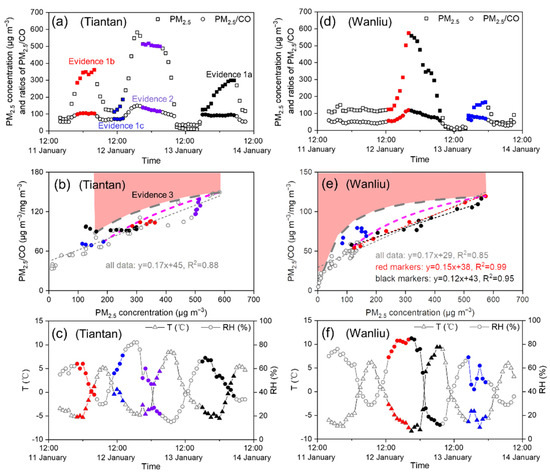
Figure 3.
Time series of hourly average mass concentrations of PM2.5 and PM2.5/CO ratios in µg m−3/mg m−3 (a), and their correlation (b) and time series of the hourly average of T and RH (c) on 9–13 January 2019 in Tiantan; (d–f) correspond to (a–c), respectively, with the location changed to Wanliu; different colors of full markers (a–f) represent data measured at different times; empty markers represent the remaining data; gray dashed line represents the theoretical dilution curve using the approach presented in the text during the decreasing period, red shallow area represents the theoretical dilution area in the presence of ambient FSPM, pink line represents the theoretical mixing curve during the increasing period as discussed in the text.
(1) Evidence 1a: The hourly averages of the PM2.5 increased by 137% from 18:00 on 13 January (PM2.5 = 126 µg m−3 at 18:00–18:59) to 05:00 on 14 January (PM2.5 = 299 µg m−3 at 05:00–05:59), with almost invariant ratios of the PM2.5/CO around 93 ± 2 µg m−3/mg m−3 (median value ± standard deviation, 2/93 ≈ 2.2%; see the black markers in Figure 3a). This indicates that the largely increased levels of the PM2.5 were probably caused solely by the accumulation of air pollutants. At 2–7 h immediately before the increase in the PM2.5 (that is, 12:00–16:00 on 13 January), the hourly averages of the PM2.5 and the ratios of the PM2.5/CO stood on a relatively low and stable platform and fluctuated narrowly around 11 ± 0.8 µg m−3 (average value ± standard deviation) and 37 ± 3 µg m−3/mg m−3, respectively. It took 2 h for the ratio to jump from the low platform (37 ± 3) to the high platform (93 ± 2), with a clear 1 h transition at 17:00 on 13 January (PM2.5/CO = 54 µg m−3/mg m−3). The extreme increase in the rate of the ratios solely during these 2 h (but not before or after) clearly reflects a rapid replacement process of the cleaner ambient air by the polluted air mass rather than by any detectable contribution from the ambient FSPM. In the replacement process, an excellent correlation was observed between the two variables, that is, PM2.5/CO = 0.54 × PM2.5 + 29, R2 = 0.998 (p < 0.05) when the data at 16:00 (start), 17:00 (middle), and 18:00 (end) were used.
(2) Evidence 1b: A similar process recurred from 22:00 on 11 January to 04:00 on 12 January (red marker in Figure 3a) when the PM2.5/CO stood on the platform of 104 ± 3 µg m−3/mg m−3 (3/104 = 2.8%) with an increase in the hourly average of the PM2.5 by 27%, that is, from 285 to 362 µg m−3. The increase in the PM2.5 was also probably determined solely by accumulation. At 3–7 h before the accumulation (from 16:00 to 19:00 on 11 January), the hourly averages of the PM2.5 and the ratios of the PM2.5/CO stood on a low platform, narrowly fluctuating around 75 ± 5 µg m−3 and 54 ± 1 µg m−3/mg m−3 (1/54 = 1.9%), respectively. The PM2.5/CO took 3 h to jump on the higher platform of 104 ± 3 µg m−3/mg m−3, but no detectable ambient FSPM can be observed before 19:00 and after 22:00 on 11 January. The replacement alone was responsible for the excellent correlation between two variables, that is, PM2.5/CO = 0.22 × PM2.5 + 40, R2 = 0.94 (p < 0.05) when the data at 19:00 (start), 20:00 (middle), 21:00 (middle), and 22:00 (end) were used.
The meteorological conditions for the time periods examined in Evidence 1a and 1b (Figure 3c) were a higher ambient relative humidity (RH > 60%) and a lower ambient temperature (T < −4 °C). The wind speed fluctuated approximately 1 m·s−1 (Supplementary Materials Figure S7a–b), favoring the accumulation of air pollutants. In addition, no precipitation was recorded between 11 and 14 January (Supplementary Materials Figure S7c).
(3) Evidence 1c: When similar meteorological conditions recurred in the late afternoon on 12 January (Figure 3c and Supplementary Materials Figure S7a–d) with an even higher ambient RH lasting for a longer time, a longer process including the accumulation, replacement, and evaporation of the PM2.5 was observed from 11:00 on 12 January to 08:00 on 13 January. The accumulation was first observed from 11:00 to 14:00 on 12 January (blue markers in Figure 3a), leading to a large increase in the PM2.5 by 63%, that is, from 114 to 186 µg m−3. However, the PM2.5/CO fluctuated narrowly around 71 ± 2 µg m−3/mg m−3 (2/71 = 2.8%).
(4) Evidence 2: The observation commenced at 21:00 on 12 January and ended at 03:00 on 13 January (purple markers in Figure 3a). During this period, the hourly averages of the PM2.5 fluctuated narrowly around 507 ± 6 µg m−3 (6/507≈1%), indicating no detectable ambient FSPM. In contrast, the ratios of the PM2.5/CO decreased by 16%, that is, from 139 to 116 µg m−3/mg m−3 with CO accumulation. On the PM2.5 platform, the decreasing ratios of the PM2.5/CO were likely caused by a fraction of semi-volatile species evaporating from the PM2.5 under the condition of decreased ambient RH (Figure 3c), and the evaporation effect seemingly canceled out the accumulation effect of the PM2.5.
(5) Evidence 3: We further plotted a theoretical dilution curve in Figure 3b (gray dashed line), assuming that the most polluted plume (that is, PM2.5 = 583 µg m−3 and PM2.5/CO = 149 µg m−3/mg m−3 observed at 19:00 on 12 January) was physically diluted by the moderately polluted plume at the end of the dilution (that is, PM2.5 = 158 µg m−3 and PM2.5/CO = 88 µg m−3/mg m−3 observed at 08:00 on 13 January) in the absence of ambient FSPM and new emissions. Assuming that the ambient FSPM took place during the dilution period, the predicted values would be distributed throughout the red shadowed area in Figure 3b above the theoretical dilution curve. This is untrue, and the null hypothesis, that is, the detectable contribution from the ambient FSPM to the increased PM2.5, was thus rejected. The theoretical replacing curve during the increasing period is also presented in Figure 3b (pink dashed line with two endpoints at the maximum PM2.5 and PM2.5/CO, and the smaller values obtained at 14:00 on 12 January). The observed values generally stood on the curve, allowing us to reject the null hypothesis.
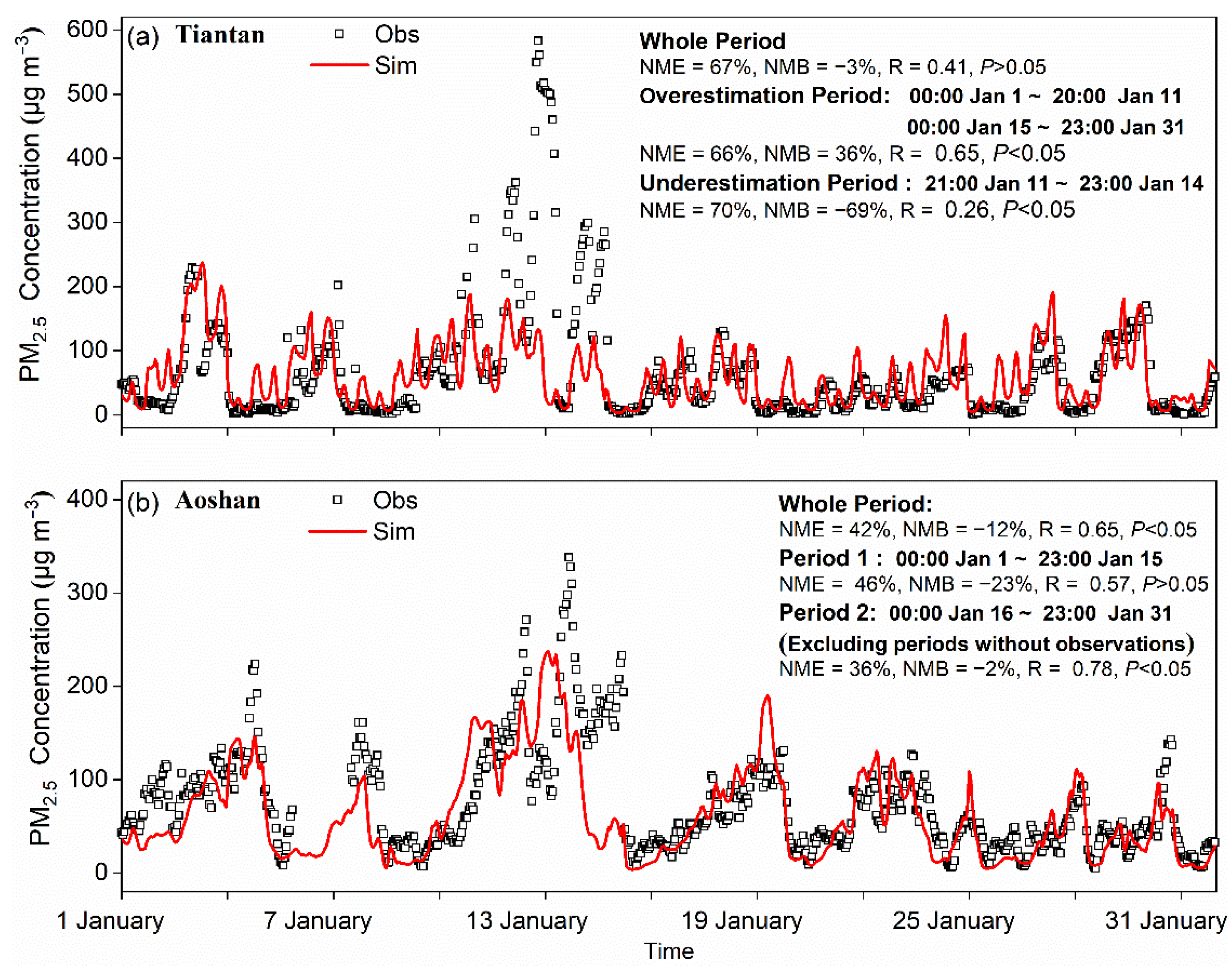
(6) Evidence 4: The CMAQ modeling results were further compared with the observations at the Tiantan site on 1–31 January 2019 (Figure 4a). The NME and NMB were 67 and −3%, respectively, indicating that the modeling performance was acceptable according to the US EPA recommended evaluation standards [41]. However, the modeling results were clearly classified into two periods, i.e., an overestimation period covering from 00:00 on 1 January to 20:00 on 11 January and from 00:00 on 15 January to 23:00 on 31 January of 2019 (NME = 66% and NMB = 36%), and an underestimation period covering from 21:00 on 11 January to 18:00 on 14 January of 2019 (NME = 70% and NMB = −69%). Combining the positive NMB during the overestimation period and the largely negative NMB during the underestimation period allows to infer missing mechanisms of the fast formation of the PM2.5 during the underestimation period [13,14,15,16,18], when the missing mechanisms overwhelmingly determined the concentrations of the PM2.5. The similar comparison results can be obtained in Qingdao (Figure 4b), and we will return to this later.
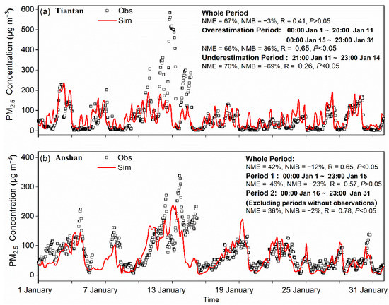
Figure 4.
The comparison of measured and simulated concentrations of PM2.5 at Tiantan in Beijing and Aoshan in Qingdao during January 2019.
(7) Additional evidence: On 12–13 January, at the Wanliu site in Beijing, a negligible contribution from the ambient FSPM to the largely increased PM2.5 was also confirmed during the pollution event (Figure 3d–f) and is further discussed in Supporting Information. The negligible contribution from the ambient FSPM can be confirmed during the events when the analysis was applied to the measurements at other sites in Beijing, shown in Supplementary Materials Figure S6a–e.
The negligible contribution from the ambient FSPM to the largely increased PM2.5 was confirmed in Langfang (~50 km south of Beijing; Supplementary Materials Figure S5a–b) and the analysis was detailed in Supporting Information. The contribution from the ambient FSPM to the significant increase in the PM2.5 was also too weak to be detectable in Baoding (~140 km southwest of Beijing, Figure 2j) on 9–13 January. The maximum value (PM2.5 = 507 µg m−3) occurred at 08:00 on 12 January in Baoding, which was 12–13% smaller than the maximum values observed at the Taintan and Wanliu sites in Beijing 11–12 h later. The PM2.5/CO corresponding to the maximum concentration of the PM2.5 in Baoding was only 77 µg m−3/mg m−3 and approximately half of the values at the two sites in Beijing. The events in Baoding are further detailed as below.
The hourly averages of the PM2.5 increased largely by 408% from 13:00 on 9 January (PM2.5 = 49 µg m−3) to 07:00 on 11 January (PM2.5 = 249 µg m−3) with the ratios of the PM2.5/CO, which fluctuated around 60 ± 6 µg m−3/mg m−3 (6/60 = 10%), with no increasing trend. The ratios of the PM2.5/CO even narrowed at approximately 61 ± 4 µg m−3/mg m−3 (4/61 = 6.6%, red markers in Figure 2j), excluding the data measured at 05:00–13:00 on 10 January. After 07:00 on 11 January, with a several-hour transition, the ratios of the PM2.5/CO reached a higher level (black markers) and fluctuated narrowly at approximately 87 ± 4 µg m−3/mg m−3 (4/87 = 4.6%). On the higher level, the hourly averages of the PM2.5 increased largely by 85% (from 267 to 495 µg m−3) and then decreased by 26% (from 495 to 361 µg m−3). The increase and decrease in the hourly average of the PM2.5 are probably caused by the accumulation effect and the dilution effect, with a negligible contribution from the ambient FSPM. When the concentration of the PM2.5 increased by 15% from 04:00 (PM2.5 = 441 µg m−3) to 08:00 on 12 January (PM2.5 = 506 µg m−3), the ratios of the PM2.5/CO stood on another platform and fluctuated narrowly around 76 ± 2 µg m−3/mg m−3 (2/76 = 2.6%, green markers). The increase in the hourly average of the PM2.5 was also probably caused by the accumulation alone. Overall, the switch of the three platforms, but with invariant ratios of the PM2.5/CO inside each, should reflect the replacement of different plumes. Based on the analysis of a negligible increase in the PM2.5/CO driven by the ambient FSPM in Baoding, the negligible ambient FSPM was also expected during the long-range transport of the polluted air masses from Baoding to downwind zones.
To examine whether the contribution from the ambient FSPM to the largely increased PM2.5 has always been too weak to be detectable in northern China, the observational results on 13–14 January in Qingdao, approximately 500 km southeast of Beijing (see maps in Supplementary Materials Figures S1 and S3), were studied (Figure 5a–g).
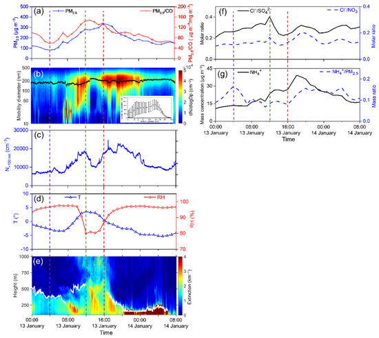
Figure 5.
Temporal variations in different variables on 13–14 January 2019 in Qingdao, China: (a) time series of hourly average mass concentrations of PM2.5 and PM2.5/CO ratios in µg m−3/mg m−3; (b) contour plot of particle number concentration (dN/dlogDp), and particle size distribution during 4:00–12:00 on 13 January, black line represents GMMD of accumulation mode; (c) time series of N>100 nm; (d) time series of T and RH; (e) planetary boundary layer height (white line) and extinction of aerosols based on the radar signal; (f) time series of molar ratios of SO42−/Cl− and NO3−/Cl−; and (g) time series of NH4+ concentrations in PM2.5 and ratios of mass NH4+/PM2.5.
3.2. Evidence for Negligible FSPM during Severe PM2.5 Air Pollution in Coastal Atmospheres
On 13 January, the hourly averages of the PM2.5 increased by 243% from 04:00 (purple dashed line, PM2.5 = 82 µg m−3) to 12:00 (green dashed line, PM2.5 = 281 µg m−3; Figure 5a) in Qingdao. At the same period, the ratios of the PM2.5/CO increased by 148%. However, the geometric median mode diameter (GMMD) of the accumulation mode particle (>100 nm) number concentration fitted by log-normal functions exhibited a stepwise change, that is, it fluctuated narrowly around 175 ± 8 nm from 00:00 to 07:41, stepping down to a platform around 158 ± 8 nm from 07:42 to 11:08, and returning to a platform around 178 ± 12 nm from 11:09 to 12:59 (black line in Figure 5b). A lack of detectable growth in the size of the accumulation mode particles allowed us to confirm that there was no detectable gas–particle condensation formation of particle matter [19,22]. Alternatively, the number concentration of atmospheric particles with diameters larger than 100 nm (N>100 nm) increased (Figure 5c) with increasing mass concentrations of the PM2.5. The two variables exhibited a moderately good correlation (R2 = 0.81, p < 0.01; Supplementary Materials Figure S8a). The good correlation together with a lack of the detectable accumulation mode particle growth in size strongly suggested that the accumulation solely caused the largely increased levels of the PM2.5.
The particles primarily emitted from coal combustion in China reportedly consist of appreciable chloride salts as well as sulfate and nitrate salts [28,42,43]. Similar to biomass burning and sea-salt aerosols, chloride is expected to be replaced by secondarily formed nitrate and sulfate in aerosol aging processes [44,45] and chloride depletion would consequently lead to a decrease in the molar ratios of Cl−/SO42− and/or Cl−/NO3−. However, both the ratios of the Cl−/SO42− and Cl−/NO3− increased with increasing concentrations of Cl−, SO42−, and NO3− during the PM2.5 increasing period (Figure 5a,f), allowing us to reject the null hypothesis of a detectable contribution from ambient FSPM to largely increase the PM2.5. Moreover, the mass ratios of the NH4+/PM2.5 exhibited a decreasing trend during the PM2.5 increasing period (Figure 5a, g). This implies that there is an increasing contribution from non-ammonium aerosols, for example, carbonaceous species, which are mainly derived from primary combustion emissions [3,36,42].
During the period of the PM2.5 increase from 04:00–12:00, the PM2.5 exhibits an excellent correlation with the PM2.5/CO, that is, [PM2.5/CO] = 0.42 × [PM2.5] + 25, R2 = 0.98, p < 0.01 (Supplementary Materials Figure S8b) as the slightly polluted plume was replaced by the heavily polluted plume. From 13:00 to 16:00, the PM2.5/CO decreased by 9% (that is, from 149 to 136 µg m−3/mg m−3), while the concentration of the PM2.5 increased by 22% (that is, from 277 to 338 µg m−3). The GMMD of the accumulation mode (Figure 5b) slightly decreased by ~30 nm with increasing N>100 nm (Figure 5c) during this period. This indicates that the accumulation was accompanied by the evaporation of semi-volatile species from the particles to some extent, supported by decreasing ratios of Cl−/SO42− and Cl−/NO3−, similar to Scenario E in Figure 2e. This was caused by the increase in the mixing layer based on the observed radar signals (Figure 5e) and meteorological conditions (Figure 5d and Supplementary Materials Figure S9a–c).
The CMAQ modeling results were also evaluated against the observations at the Aoshan site in Qingdao on 1–31 January 2019 (Figure 4b). The calculated NMB and NME indicated an acceptable modeling performance according to the US EPA recommended evaluation standards [41]. However, a worsened modeling performance accompanied by increased PM2.5 concentrations can be found during the first-half period than in the second-half period, i.e., NME = 46 %, NMB = −23 %, and R = 0.57 (first-half period) versus NME = 36 %, NMB = −2 %, and R = 0.78 (second-half period). An even worsened modeling performance and larger underestimation of the PM2.5 concentrations occurred during the period from 04:00 on 13 January to 05:00 on 15 January with an NMB as low as −49 %, when high concentrations of the PM2.5 were observed. Missing mechanisms of the fast formation of the PM2.5 may also overwhelmingly determine the concentrations of the PM2.5 during the short period.
Overall, the ambient FSPM is confirmed to be too weak to contribute to largely increased PM2.5 during severe PM2.5 pollution events at various locations on different days in northern China. To meet the law of mass conservation, a mechanism that can generate mass concentrations of PM2.5 exceeding the observations was required to interpret the event by considering evaporation and dispersion of PM2.5 in the ambient air.
4. Discussion
4.1. Impractical Conversion Rate of SO2 to SO42− Absence of Non-Precipitation Cloud during the Events
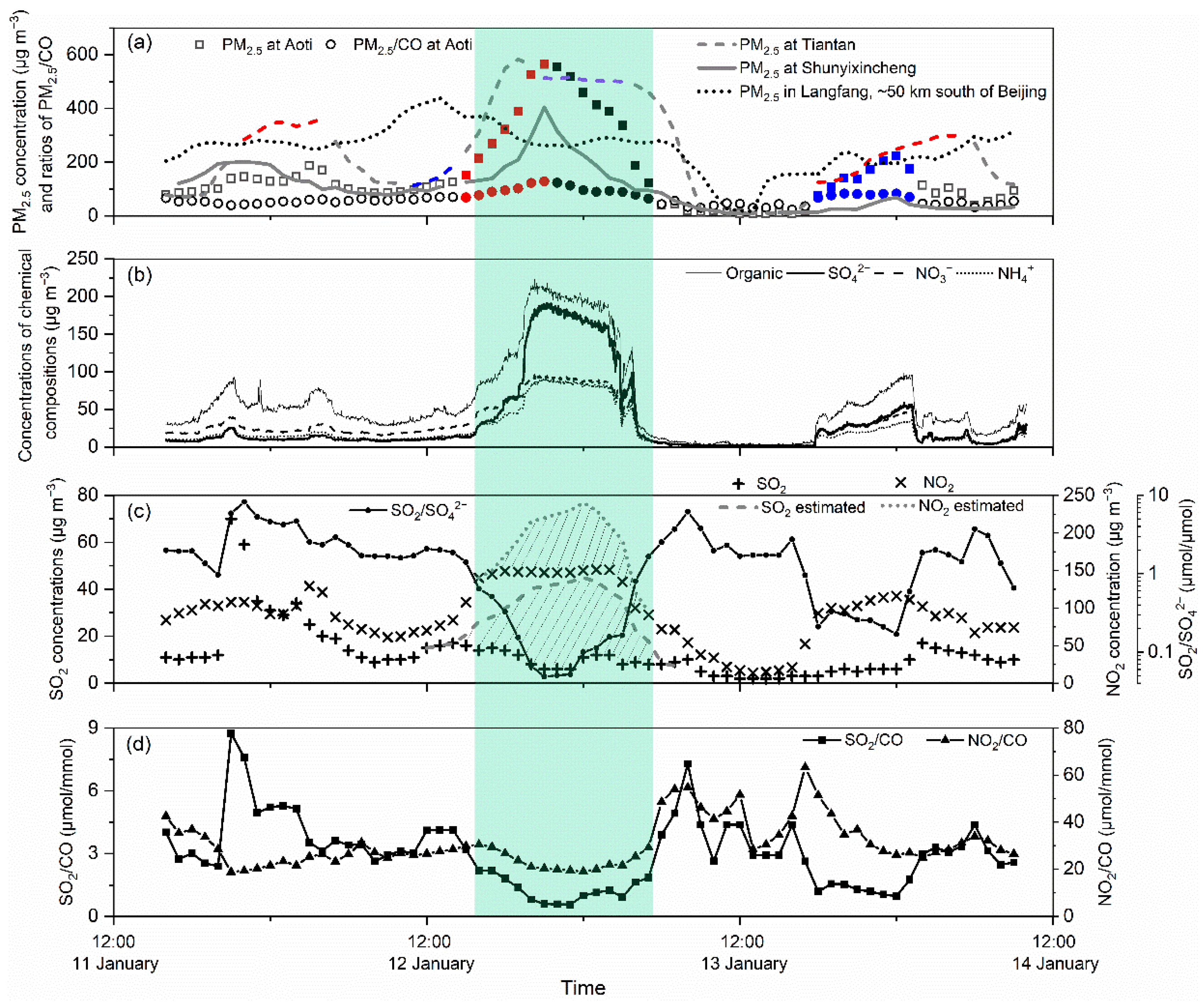
To study the chemical formation of secondary ions such as SO42−, NO3−, and NH4+ in the PM2.5, the chemical components in the PM2.5 measured at the U-site and the routine air quality observations at the nearby Aoti site were combined during the events (Figure 6a–d). At the Aoti site, the PM2.5 concentrations increased from 118 ± 9 µg m−3 at 12:00–14:00 to 548 ± 20 µg m−3 at 20:00–22:00 on 12 January when the concentrations of the SO42−, NO3−, NH4+, and organics in the PM2.5 at the U-site increased by 169, 66, 72, and 159 µg m−3, respectively (Figure 6a–b). The large increase in the SO42− concentrations led to the mass ratio of (SO42− + NO3− + NH4+) to organics that were as high as 1.6 ± 0.2 from 16:00 on 12 January to 05:00 on 13 January (blue shadow in Figure 6b), contrasting to 1.1 ± 0.2 from 16:00 on 11 January to 09:00 on 14 January by excluding the blue shadow period. Thus, we further calculated the conversion rate of SO2 to SO42− during the blue shadow period. Suppose that no ambient conversion of SO2 to SO42− occurred, the ratios of the SO2/CO should be constant through the blue shadow period. Thus, the ratios of the SO2/CO at the initial few hours, i.e., 4.1 ± 0.0 µg m−3/mg m−3 at 12:00–14:00 on 12 January, were combined with the CO concentrations measured afterward to estimate the theoretically accumulated SO2 concentration absent of secondary conversions (dashed line in Figure 6c). The difference between the dashed line and the observed concentrations of SO2 (black cross) can be the assumed converted amount of SO2 to SO42− and the conversion rate of the SO2 was as high as 55% per hour during the increasing period from 12:00–14:00 to 20:00–22:00 on 12 January. Even with such high conversion rates, the converted SO2 can only account for ~30% of the increased SO42− concentrations in the PM2.5 during the increasing period. In this case, an additional hypothesis was required to interpret the lack of the mass conservation between the increased concentrations of SO42− in the PM2.5 and the theoretically converted SO2, i.e., (1) the ratio of the SO2/CO near the SO2 sources should be larger than 4.1 ± 0.0 µg m−3/mg m−3; (2) when the SO2 transported from the sources to the observational site, a large fraction of sticky SO2 has been scavenged through atmospheric deposition; (3) however, it is not the case for the SO42− in the PM2.5 because of its smaller deposition velocity. In the absence of the non-precipitation-cloud processing conversion of the SO2, such high conversion rates were practically impossible according to previously reported results in combustion plumes [46,47,48,49]. The same analysis can be applied to the conversion of NO2 to particulate NO3− as shown in Figure 6c. The 11% conversion of NO2 to NO3− per hour during the increasing period was also practically impossible absent of the non-precipitation-cloud processing conversion of NO2.
Figure 6.
Temporal variations in different variables on 11–14 January 2019 at the Aoti site: (a) time series of hourly average mass concentrations of PM2.5 at the Aoti site in comparison with those observed at the Tiantan and Shunyixincheng site, and in Langfang, and PM2.5/CO ratios in µg m−3/mg m−3 at the Aoti site; (b) time series of organic, SO42–, NO3–, and NH4+ concentrations in PM2.5 at the U-site; (c) time series of SO2 or theoretically accumulated SO2 (gray short dotted line) and NO2 or theoretically accumulated NO2 (gray short dashed line) concentrations and molar ratios of SO2/SO42−, the upper and lower shadow area represents the theoretically converted amounts of NO2 and SO2 to NO3− and SO42−, respectively; (d) time series of molar ratios of SO2/CO and NO2/CO.
In addition, the different temporal variation patterns of the PM2.5 mass concentration at various sites in Beijing (Figure 6a) suggested that the local sources rather than the long-range transport of air pollutants caused the event. The analysis was also supported by the spatial heterogeneity of the PM2.5/CO during the blue shadow period. For example, the PM2.5/CO corresponding to the maximum concentration of the PM2.5 reached 149 µg m−3/mg m−3 at the Tiantan site and occurred at 19:00 on 12 January (Figure 3a). One hour later, the maximum PM2.5/CO of 120 µg m−3/mg m−3 occurred at the Wanliu site (Figure 3d). Two hours later, the maximum PM2.5/CO simultaneously occurred at the Aoti (128 µg m−3/mg m−3) and Shunyixincheng (104 µg m−3/mg m−3), although there was 38 km between the two sites. Although the long-range transport from the south, e.g., Langfang, to Beijing cannot be completely excluded, the maximum value of the PM2.5 in Langfang was only 438 µg m−3 and occurred at 13:00 on 12 January. The PM2.5/CO corresponding to the maximum concentration of the PM2.5 in Langfang was 117 µg m−3/mg m−3, which was almost the same as the corresponding maximum value of 120 µg m−3/mg m−3 at the Wanliu site. However, the maximum value was 24% smaller than that observed at the Tiantan site in Beijing.
4.2. Hypothesis for In-Fresh-Stack-Plume Non-Precipitation-Cloud Processing of Aerosols
Figure 1a shows that the in-fresh-stack-plume non-precipitation-cloud processing of aerosols includes several processes: (1) the rapid cooling of water vapor immediately after the plume leaves the stack, leading to the formation of water droplets similar to a non-precipitation cloud (Figure 1d); (2) highly concentrated air pollutants would experience non-precipitation-cloud processing of aerosols, including the fast chemical conversion of air pollutants in droplets, and the evaporation of droplets to generate aerosols with largely decreasing liquid water content afterward [46,47,48,49,50,51,52,53]; (3) freshly processed aerosols would experience further evaporation, with the plumes to be diluted, if the aerosols include semi-volatile species such as NH4NO3 and small molecular weight organics [42]. The Hoppel effect is the direct result of the non-precipitation-cloud processing of secondary aerosols [50], leading to an accumulation mode (100–200 nm) of particle number concentration and a trough at 50–100 nm in the particle number concentration spectra (Figure 1b). No measurements in the stack plumes during the extreme events were available in this study. The non-precipitation-cloud processing of aerosols in the stack plumes can clearly be seen during the observations shown in Figure 1b, the data of which were measured by an unmanned aerial vehicle equipped with a particle sizer flying through the in-fresh-stack-plume non-precipitation cloud (Figure 1c–d). In the ambient air near the ground level during the unmanned aerial vehicle observational period, the Aitken mode particles dominated the particle number size spectra with the GMMD of Aitken mode particles at 50–60 nm (Figure 1b). In the stack plumes, the accumulation mode particles dominated the particle number size spectra with a trough in 50–100 nm. More details on the unique measurement can be found in Supporting Information.
The non-precipitation-cloud processing rate of secondary aerosols, for example, sulfate aerosols, is commonly assumed to be approximately two orders of magnitude faster than that in ambient air without the processing of aerosols [52]. The in-fresh-stack-plume non-precipitation-cloud processing of aerosols should have an even higher formation rate of secondary aerosols than in ambient air because of the high concentrations of air pollutants in plumes. For example, the lower limit values of SO2 were 200, 100, and 50 mg·m−3 for coal burning, oil burning, and gas-fired boilers, respectively, based on the emission standards of air pollutants in China (GB13271-2014). The three limit values were 200, 200, and 150 mg·m−3 for NOx. The limit values of SO2 and NOx in the plumes were approximately three to four orders of magnitude higher than their concentrations in the ambient air in northern China [8,15,18,42]. Thus, assuming that the production rates of particulate chemicals via in-fresh-stack-plume non-precipitation clouds are three to four orders of magnitude higher than those of ambient air, it can be roughly estimated that 1 min of processing would generate aerosols equal to that generated via ambient FSPM continuing for tens of hours to several days, particularly considering the role of NO2 in chemical reactions [16,17,22]. The lifetime of non-precipitation cloud droplets in fresh stack plumes seems critical to determine the amount of processed aerosols, but the processing needs further evaluation to be included in air quality models.
Based on our observations, the cloud droplets from community house-heating stacks normally survive 20–30 s under wind speeds of 2–4 m s−1 (Supplementary Materials Video S1). The lifetime of the non-precipitation cloud droplets depends on the amount of water vapor released from the stacks and the ambient conditions. High ambient RH, low ambient temperature, and stagnant weather conditions would prolong the lifetime of in-fresh-stack-plume cloud droplets from dozens of seconds to five minutes (Supplementary Materials Videos S2–4, the lifetime was counted manually and from the plume emitted from the outlet to the disappearance), generate extremely high concentrations of PM2.5 within minutes, and largely increase the PM2.5/CO ratios through fast conversion of air pollutants therein. However, the lifetime was only approximately 15 s at high wind speed and low RH (Supplementary Materials Video S5).
5. Implications
In the literature, all novel hypotheses to be proposed are based on two key issues: (1) the fast conversion of chemicals was required to generate high concentrations of the PM2.5 during the extreme events, (2) but no natural cloud was present in the planetary boundary layer and thereby no rapid generation of the PM2.5 through the cloud processing of aerosols was expected [1,3,5,6,7,16,17,18,19,20,21,22]. The fast conversion was thereby conventionally called the “missing formation mechanism”. The non-precipitation-cloud processing of aerosols, however, always occurs in fresh combustion plumes during the extreme events. In addition, the non-precipitation-cloud processing of aerosols can be largely enhanced under high ambient RH, low ambient temperature, and stagnant weather conditions with the prolonged lifetime of water droplets in fresh plumes. To prevent extreme PM2.5 pollution events in the future, environment-friendly measures are needed to reduce the water vapor released from stacks in China.
Supplementary Materials
The following are available online at https://www.mdpi.com/article/10.3390/atmos13050673/s1, Figure S1: Map of Beijing, Langfang, Baoding, and Qingdao in China; Figure S2: Map of Wanliu, Aoti, Tiantan, Shunyixincheng, and U-site in Beijing; Figure S3: Map of three sampling sites, (1) Pilot National Laboratory for Marine Science and Technology (Qingdao), (2) a local air quality monitoring station at Aoshan, (3) an air quality monitoring supersite in Qingdao; Figure S4: The two domains of meteorological modeling system: Domain 1, a mother domain containing 164 × 97 grid cells at a 36 km spatial resolution for China, and Domain 2, a sub-domain containing 142 × 220 grid cells at a 12 km resolution for eastern China; Figure S5: Time series of hourly averages and the ratios of PM2.5/CO in µg m−3/mg m−3 (a) and their correlation (b) on 9–13 January 2019 in Langfang, different color represents specific periods. Red full markers represent data from 21:00 on 9 January to 10:00 on 10 January; pink full markers represent data from 14:00 on 10 January to 01:00 on 11 January; orange full markers represent data from 03:00–12:00 and 14:00–15:00 on 11 January; blue half markers represent data from 18:00 on 11 January to 07:00 on 12 January; green half markers represent data from 19:00 on 12 January to 06:00 on 13 January; empty markers represent the data measured other times; Figure S6: Time series of hourly average mass concentrations of PM2.5 measured at nine additional sites in Beijing on 11–14 January 2019; Figure S7: Time series of hourly averages of WS, WD, precipitation, and low cloud percentage at the stations close to Tiantan (a–d) and close to Wanliu (e,f) in Beijing on 11–14 January 2019; Figure S8: Correlations of N>100 and ratios of PM2.5/CO in µg m−3/mg m−3 with hourly average mass concentrations of PM2.5; N>100 nm (a) and PM2.5/CO (b), gray full markers represent data during the decreasing period of PM2.5 from 16:00 on 13 January to 04:00 on 14 January; gray dash line represents the theoretical dilution curve using the approach presented in the text, red shallowed area represents the theoretical dilution area in the presence of ambient FMSP; red full markers represent data during the increasing period of PM2.5 at 04:00–12:00 on 13 January; pink dash line represents the theoretical mixing curve; empty markers represent the data measured at other times; Figure S9: Time series of hourly averages of WS, WD, and precipitation recorded at Aoshan monitoring station in Qingdao; Figure S10: The mean size distributions of particle number concentrations measured by SMPS mounted on UAV in IDSPs and ambient air; Video S1: The video was taken on 24 November 2020 in Qingdao, China. The cloud droplets from community house-heating stacks normally survive approximately 20–30 s. The 3 h average RH, wind speed, and T were 54%, 1.7 m/s, and 4 ℃, respectively, after observing the plume; Video S2: The video was taken on 2 December 2020 in Qingdao, China. The cloud droplets from community house-heating stacks normally survive approximately 40–50 s. The weather was rainy and the 3 h average RH, wind speed, and T were 92%, 1.7 m/s, and 2 ℃, respectively, after observing the plume; Video S3: The video was taken on 27 December 2020 in Qingdao, China. The cloud droplets from community house-heating stacks normally survive approximately 1 min 50 s. The 3 h average RH, wind speed, and T were 87 %, 1.0 m/s, and 8 ℃, respectively, after observing the plume; Video S4: The video was taken on 28 December 2020 in Qingdao, China. The cloud droplets from community house-heating stacks normally survive approximately 5 min. The 3 h average RH, wind speed, and T were 89 %, 1.0 m/s, and 7 ℃, respectively, after observing the plume; Video S5: The video was taken on 25 November 2020 in Qingdao, China. The cloud droplets from community house-heating stacks survive approximately 15 s. The 3 h average RH, wind speed, and T were 42%, 1.3 m/s, and 8 ℃, respectively, after observing the plume; Video S6: A nano-Scan Particle Sizer on an Unmanned Aerial Vehicle developed in 2017 was used to monitor the particle formation in fresh stack combustion plumes.
Author Contributions
Conceptualization, X.Y.; data curation, Y.S. (Yanjie Shen), H.M. and X.Y.; formal analysis, Y.S. (Yanjie Shen), H.M. and X.Y.; funding acquisition, X.Y.; investigation, Y.S. (Yanjie Shen), H.M. and X.Y.; methodology, Y.S. (Yanjie Shen), H.M. and X.Y.; project administration, X.Y.; resources, Y.S. (Yanjie Shen) and H.M.; software, Y.S. (Yanjie Shen), H.M. and X.Y.; supervision, X.Y.; validation, Y.S. (Yanjie Shen), H.M. and X.Y.; visualization, X.Y.; writing—original draft, Y.S. (Yanjie Shen), H.M. and X.Y.; writing—review and editing, Y.S. (Yanjie Shen), H.M., X.Y., Z.P., Y.S. (Yele Sun), J.Z., Y.G., L.F., X.L. and H.G. All authors have read and agreed to the published version of the manuscript.
Funding
This research was funded by the National Natural Science Foundation of China, grant number 41776086, and the National Key Research and Development Program of China, grant number 2016YFC0200500.
Institutional Review Board Statement
Not applicable.
Informed Consent Statement
Not applicable.
Data Availability Statement
Not applicable.
Conflicts of Interest
The authors declare no conflict of interest. The funders had no role in the design of the study; in the collection, analyses, or interpretation of data; in the writing of the manuscript; or in the decision to publish the results.
References
- An, Z.; Huang, R.J.; Zhang, R.; Tie, X.; Li, G.; Cao, J.; Zhou, W.; Shi, Z.; Han, Y.; Gu, Z.; et al. Severe haze in northern China: A synergy of anthropogenic emissions and atmospheric processes. Proc. Natl. Acad. Sci. USA 2019, 116, 8657–8666. [Google Scholar] [CrossRef] [PubMed] [Green Version]
- Cai, S.; Wang, Y.; Zhao, B.; Wang, S.; Chang, X.; Hao, J. The impact of the “Air Pollution Prevention and Control Action Plan” on PM2.5 concentrations in Jing-Jin-Ji region during 2012–2020. Sci. Total Environ. 2017, 580, 197–209. [Google Scholar] [CrossRef] [PubMed]
- Chan, C.K.; Yao, X. Air pollution in mega cities in China. Atmos. Environ. 2008, 42, 1–42. [Google Scholar] [CrossRef]
- Chang, W.; Zhan, J.; Zhang, Y.; Li, Z.; Xing, J.; Li, J. Emission-driven changes in anthropogenic aerosol concentrations in China during 1970–2010 and its implications for PM2.5 control policy. Atmos. Res. 2018, 212, 106–119. [Google Scholar] [CrossRef]
- Chen, Z.; Chen, D.; Wen, W.; Zhuang, Y.; Kwan, M.-P.; Chen, B.; Zhao, B.; Yang, L.; Gao, B.; Li, R.; et al. Evaluating the “2 + 26” regional strategy for air quality improvement during two air pollution alerts in Beijing: Variations in PM2.5 concentrations, source apportionment, and the relative contribution of local emission and regional transport. Atmos. Chem. Phys. 2019, 19, 6879–6891. [Google Scholar] [CrossRef] [Green Version]
- Elser, M.; Huang, R.-J.; Wolf, R.; Slowik, J.G.; Wang, Q.; Canonaco, F.; Li, G.; Bozzetti, C.; Daellenbach, K.R.; Huang, Y.; et al. New insights into PM2.5 chemical composition and sources in two major cities in China during extreme haze events using aerosol mass spectrometry. Atmos. Chem. Phys. 2016, 16, 3207–3225. [Google Scholar] [CrossRef] [Green Version]
- Ji, D.; Li, L.; Wang, Y.; Zhang, J.; Cheng, M.; Sun, Y.; Liu, Z.; Wang, L.; Tang, G.; Hu, B.; et al. The heaviest particulate air-pollution episodes occurred in northern China in January, 2013: Insights gained from observation. Atmos. Environ. 2014, 92, 546–556. [Google Scholar] [CrossRef]
- Lachatre, M.; Fortems-Cheiney, A.; Foret, G.; Siour, G.; Dufour, G.; Clarisse, L.; Clerbaux, C.; Coheur, P.-F.; Van Damme, M.; Beekmann, M. The unintended consequence of SO2 and NO2 regulations over China: Increase of ammonia levels and impact on PM2.5 concentrations. Atmos. Chem. Phys. 2019, 19, 6701–6716. [Google Scholar] [CrossRef] [Green Version]
- Si, Y.; Yu, C.; Zhang, L.; Zhu, W.; Cai, K.; Cheng, L.; Chen, L.; Li, S. Assessment of satellite-estimated near-surface sulfate and nitrate concentrations and their precursor emissions over China from 2006 to 2014. Sci. Total Environ. 2019, 669, 362–376. [Google Scholar] [CrossRef]
- Sun, Y.L.; Wang, Z.F.; Du, W.; Zhang, Q.; Wang, Q.Q.; Fu, P.Q.; Pan, X.L.; Li, J.; Jayne, J.; Worsnop, D.R. Long-term real-time measurements of aerosol particle composition in Beijing, China: Seasonal variations, meteorological effects, and source analysis. Atmos. Chem. Phys. 2015, 15, 10149–10165. [Google Scholar] [CrossRef] [Green Version]
- Wang, Y.; Zhang, Q.Q.; He, K.; Zhang, Q.; Chai, L. Sulfate-nitrate-ammonium aerosols over China: Response to 2000–2015 emission changes of sulfur dioxide, nitrogen oxides, and ammonia. Atmos. Chem. Phys. 2013, 13, 2635–2652. [Google Scholar] [CrossRef] [Green Version]
- Zhao, X.J.; Zhao, P.S.; Xu, J.; Meng, W.; Pu, W.W.; Dong, F.; He, D.; Shi, Q.F. Analysis of a winter regional haze event and its formation mechanism in the North China Plain. Atmos. Chem. Phys. 2013, 13, 5685–5696. [Google Scholar] [CrossRef] [Green Version]
- Zheng, B.; Zhang, Q.; Zhang, Y.; He, K.B.; Wang, K.; Zheng, G.J.; Duan, F.K.; Ma, Y.L.; Kimoto, T. Heterogeneous chemistry: A mechanism missing in current models to explain secondary inorganic aerosol formation during the January 2013 haze episode in North China. Atmos. Chem. Phys. 2015, 15, 2031–2049. [Google Scholar] [CrossRef] [Green Version]
- Li, M.; Wang, T.; Xie, M.; Li, S.; Zhuang, B.; Huang, X.; Chen, P.; Zhao, M.; Liu, J. Formation and Evolution Mechanisms for Two Extreme Haze Episodes in the Yangtze River Delta Region of China During Winter 2016. J. Geophys. Res. Atmos. 2019, 124, 3607–3623. [Google Scholar] [CrossRef]
- Yang, Y.; Liu, X.; Qu, Y.; Wang, J.; An, J.; Zhang, Y.; Zhang, F. Formation mechanism of continuous extreme haze episodes in the megacity Beijing, China, in January 2013. Atmos. Res. 2015, 155, 192–203. [Google Scholar] [CrossRef]
- Chang, Y.; Huang, R.J.; Ge, X.; Huang, X.; Hu, J.; Duan, Y.; Zou, Z.; Liu, X.; Lehmann, M.F. Puzzling haze events in China during the coronavirus (COVID-19) shutdown. Geophys Res. Lett. 2020, 47, e2020GL088533. [Google Scholar] [CrossRef] [PubMed]
- Wang, J.; Li, J.; Ye, J.; Zhao, J.; Wu, Y.; Hu, J.; Liu, D.; Nie, D.; Shen, F.; Huang, X.; et al. Fast sulfate formation from oxidation of SO2 by NO2 and HONO observed in Beijing haze. Nat. Commun. 2020, 11, 2844. [Google Scholar] [CrossRef]
- Cheng, Y.; Zheng, G.; Wei, C.; Mu, Q.; Zheng, B.; Wang, Z.; Gao, M.; Zhang, Q.; He, K.; Carmichael, G.; et al. Reactive nitrogen chemistry in aerosol water as a source of sulfate during haze events in China. Sci. Adv. 2016, 2, e1601530. [Google Scholar] [CrossRef] [Green Version]
- Guo, S.; Hu, M.; Zamora, M.L.; Peng, J.; Shang, D.; Zheng, J.; Du, Z.; Wu, Z.; Shao, M.; Zeng, L.; et al. Elucidating severe urban haze formation in China. Proc. Natl. Acad. Sci. USA 2014, 111, 17373–17378. [Google Scholar] [CrossRef] [Green Version]
- Huang, R.J.; Zhang, Y.; Bozzetti, C.; Ho, K.F.; Cao, J.J.; Han, Y.; Daellenbach, K.R.; Slowik, J.G.; Platt, S.M.; Canonaco, F.; et al. High secondary aerosol contribution to particulate pollution during haze events in China. Nature 2014, 514, 218–222. [Google Scholar] [CrossRef] [Green Version]
- Moch, J.M.; Dovrou, E.; Mickley, L.J.; Keutsch, F.N.; Cheng, Y.; Jacob, D.J.; Jiang, J.; Li, M.; Munger, J.W.; Qiao, X.; et al. Contribution of hydroxymethane sulfonate to ambient particulate matter: A potential explanation for high particulate sulfur during severe winter haze in Beijing. Geophys. Res. Lett. 2018, 45, 11969–11979. [Google Scholar] [CrossRef] [Green Version]
- Wang, G.; Zhang, R.; Gomez, M.E.; Yang, L.; Levy Zamora, M.; Hu, M.; Lin, Y.; Peng, J.; Guo, S.; Meng, J.; et al. Persistent sulfate formation from London Fog to Chinese haze. Proc. Natl. Acad. Sci. USA 2016, 113, 13630–13635. [Google Scholar] [CrossRef] [PubMed] [Green Version]
- Guo, T.; Guo, Z.; Wang, J.; Feng, J.; Gao, H.; Yao, X. Tracer-based investigation of organic aerosols in marine atmospheres from marginal seas of China to the northwest Pacific Ocean. Atmos. Chem. Phys. 2020, 20, 5055–5070. [Google Scholar] [CrossRef]
- Man, H.; Zhu, Y.; Ji, F.; Yao, X.; Lau, N.T.; Li, Y.; Lee, B.P.; Chan, C.K. Comparison of daytime and nighttime new particle growth at the HKUST supersite in Hong Kong. Environ. Sci. Technol. 2015, 49, 7170–7178. [Google Scholar] [CrossRef] [PubMed]
- Shen, Y.; Wang, J.; Gao, Y.; Chan, C.K.; Zhu, Y.; Gao, H.; Petaja, T.; Yao, X. Sources and formation of nucleation mode particles in remote tropical marine atmospheres over the South China Sea and the Northwest Pacific Ocean. Sci. Total Environ. 2020, 735, 139302. [Google Scholar] [CrossRef] [PubMed]
- Yao, X.; Lau, N.T.; Fang, M.; Chan, C.K. Real-Time observation of the Transformation of Ultrafine Atmospheric Particle Modes. Aerosol Sci. Technol. 2005, 39, 831–841. [Google Scholar] [CrossRef]
- Feng, L.; Yang, T.; Wang, D.; Wang, Z.; Pan, Y.; Matsui, I.; Chen, Y.; Xin, J.; Huang, H. Identify the contribution of elevated industrial plume to ground air quality by optical and machine learning methods. Environ. Res. Commun. 2020, 2, 021005. [Google Scholar] [CrossRef]
- Li, Z.; Jiang, J.; Ma, Z.; Fajardo, O.A.; Deng, J.; Duan, L. Influence of flue gas desulfurization (FGD) installations on emission characteristics of PM2.5 from coal-fired power plants equipped with selective catalytic reduction (SCR). Environ. Pollut. 2017, 230, 655–662. [Google Scholar] [CrossRef]
- Wei, Y.; Chen, H.; Sun, H.; Zhang, F.; Shang, X.; Yao, L.; Zheng, H.; Li, Q.; Chen, J. Nocturnal PM2.5 explosive growth dominates severe haze in the rural North China Plain. Atmos. Res. 2020, 242, 105020. [Google Scholar] [CrossRef]
- Lonsdale, C.R.; Stevens, R.G.; Brock, C.A.; Makar, P.A.; Knipping, E.M.; Pierce, J.R. The effect of coal-fired power-plant SO2 and NOx control technologies on aerosol nucleation in the source plumes. Atmos. Chem. Phys. 2012, 12, 11519–11531. [Google Scholar] [CrossRef] [Green Version]
- Lee, S.W.; Herage, T.; Dureau, R.; Young, B. Measurement of PM2.5 and ultra-fine particulate emissions from coal-fired utility boilers. Fuel 2013, 108, 60–66. [Google Scholar] [CrossRef]
- Brock, C.A.; Washenfelder, R.A.; Trainer, M.; Ryerson, T.B.; Wilson, J.C.; Reeves, J.M.; Huey, L.G.; Holloway, J.S.; Parrish, D.D.; Hübler, G.; et al. Particle growth in the plumes of coal-fired power plants. J. Geophys. Res. 2002, 107, D12. [Google Scholar] [CrossRef]
- Marris, H.; Deboudt, K.; Augustin, P.; Flament, P.; Blond, F.; Fiani, E.; Fourmentin, M.; Delbarre, H. Fast changes in chemical composition and size distribution of fine particles during the near-field transport of industrial plumes. Sci. Total. Environ. 2012, 427, 126–138. [Google Scholar] [CrossRef]
- Mylläri, F.; Asmi, E.; Anttila, T.; Saukko, E.; Vakkari, V.; Pirjola, L.; Hillamo, R.; Laurila, T.; Häyrinen, A.; Rautiainen, J.; et al. New particle formation in the fresh flue-gas plume from a coal-fired power plant: Effect of flue-gas cleaning. Atmos. Chem. Phys. 2016, 16, 7485–7496. [Google Scholar] [CrossRef] [Green Version]
- Arya, S.P. Modeling and Parameterization of Near-Source Diffusion in Weak Winds. J. Appl. Meteorol. 1995, 34, 1112. [Google Scholar] [CrossRef]
- Lei, L.; Sun, Y.; Ouyang, B.; Qiu, Y.; Xie, C.; Tang, G.; Zhou, W.; He, Y.; Wang, Q.; Cheng, X.; et al. Vertical distributions of primary and secondary aerosols in urban boundary layer: Insights into sources, chemistry, and interaction with meteorology. Environ. Sci. Technol. 2021, 55, 4542–4552. [Google Scholar] [CrossRef]
- Zhu, Y.; Sabaliauskas, K.; Liu, X.; Meng, H.; Gao, H.; Jeong, C.-H.; Evans, G.J.; Yao, X. Comparative analysis of new particle formation events in less and severely polluted urban atmosphere. Atmos. Environ. 2014, 98, 655–664. [Google Scholar] [CrossRef]
- Teng, X.; Hu, Q.; Zhang, L.; Qi, J.; Shi, J.; Xie, H.; Gao, H.; Yao, X. Identification of major sources of atmospheric NH3 in an urban environment in Northern China during wintertime. Environ. Sci. Technol. 2017, 51, 6839–6848. [Google Scholar] [CrossRef]
- Fernald, F.G. Analysis of atmospheric lidar observations: Some comments. Appl. Opt. 1984, 23, 652–653. [Google Scholar] [CrossRef]
- Liu, X.; Chang, M.; Zhang, J.; Wang, J.; Gao, H.; Gao, Y.; Yao, X. Rethinking the causes of extreme heavy winter PM2.5 pollution events in northern China. Sci. Total Environ. 2021, 794, 148637. [Google Scholar] [CrossRef]
- US-EPA. Guidance on the Use of Models and Other Analyses for demonstrating attainment of Air Quality Goals for Ozone, PM2.5 and Regional Haze; EPA-454/B-07-002; U.S. Environmental Protection Agency: Research Triangle Park, NC, USA, 2007.
- Sun, Y.; Jiang, Q.; Wang, Z.; Fu, P.; Li, J.; Yang, T.; Yin, Y. Investigation of the sources and evolution processes of severe haze pollution in Beijing in January 2013. J. Geophys. Res. Atmos. 2014, 119, 4380–4398. [Google Scholar] [CrossRef]
- Wu, B.; Tian, H.; Hao, Y.; Liu, S.; Liu, X.; Liu, W.; Bai, X.; Liang, W.; Lin, S.; Wu, Y.; et al. Effects of wet flue gas desulfurization and wet electrostatic precipitators on emission characteristics of particulate matter and its ionic compositions from four 300 MW level ultralow coal-fired power plants. Environ. Sci. Technol. 2018, 52, 14015–14026. [Google Scholar] [CrossRef] [PubMed]
- Liu, X.; Van Espen, P.; Adams, F.; Cafmeyer, J.; Maenhaut, W. Biomass burning in Southern Africa: Individual particle characterization of atmospheric aerosols and savanna fire samples. J. Atmos. Chem. 2000, 36, 135–155. [Google Scholar] [CrossRef]
- Wu, B.; Bai, X.; Liu, W.; Lin, S.; Liu, S.; Luo, L.; Guo, Z.; Zhao, S.; Lv, Y.; Zhu, C.; et al. Non-negligible stack emissions of noncriteria air pollutants from coal-fired power plants in China: Condensable particulate matter and sulfur trioxide. Environ. Sci. Technol. 2020, 54, 6540–6550. [Google Scholar] [CrossRef] [PubMed]
- Ding, X.; Li, Q.; Wu, D.; Wang, X.; Li, M.; Wang, T.; Wang, L.; Chen, J. Direct observation of sulfate explosive growth in wet plumes emitted from typical coal-fired stationary sources. Geophys. Res. Lett. 2021, 48, e2020GL092071. [Google Scholar] [CrossRef]
- Dittenhoefer, A.C.; De Pena, R.G. Sulfate aerosol production and growth in coal-operated power plant plumes. J. Geophys. Res. Ocean. 1980, 85, 4499–4506. [Google Scholar] [CrossRef]
- Green, J.R.; Fiddler, M.N.; Holloway, J.S.; Fibiger, D.L.; McDuffie, E.E.; Campuzano-Jost, P.; Schroder, J.C.; Jimenez, J.L.; Weinheimer, A.J.; Aquino, J.; et al. Rates of wintertime atmospheric SO2 oxidation based on aircraft observations during clear-sky conditions over the Eastern United States. J. Geophys. Res. Atmos. 2019, 124, 6630–6649. [Google Scholar] [CrossRef]
- Luria, M.; Imhoff, R.E.; Valente, R.J.; Parkhurst, W.J.; Tanner, R.L. Rates of conversion of sulfur dioxide to sulfate in a scrubbed power plant plume. J. Air Waste Manag. Assoc. 2001, 51, 1408–1413. [Google Scholar] [CrossRef] [Green Version]
- Hoppel, W.A.; Frick, G.M.; Fitzgerald, J.W. Deducing droplet concentration and supersaturation in marine boundary layer clouds from surface aerosol measurements. J. Geophys. Res. Atmospheres 1996, 101, 26553–26565. [Google Scholar] [CrossRef]
- Leng, C.-B.; Roberts, J.E.; Zeng, G.; Zhang, Y.-H.; Liu, Y. Effects of temperature, pH, and ionic strength on the Henry’s law constant of triethylamine. Geophys. Res. Lett. 2015, 42, 3569–3575. [Google Scholar] [CrossRef]
- Seinfeld, J.H.; Pandis, S.N. Atmospheric Chemistry and Physics: From Air Pollution to Global Climate, 3rd. ed.; Wiley: New York, NY, USA, 1997. [Google Scholar]
- Yao, X.; Zhang, L. Chemical processes in sea-salt chloride depletion observed at a Canadian rural coastal site. Atmos. Environ. 2012, 46, 189–194. [Google Scholar] [CrossRef]

Publisher’s Note: MDPI stays neutral with regard to jurisdictional claims in published maps and institutional affiliations. |
© 2022 by the authors. Licensee MDPI, Basel, Switzerland. This article is an open access article distributed under the terms and conditions of the Creative Commons Attribution (CC BY) license (https://creativecommons.org/licenses/by/4.0/).