Abstract
A high-resolution simulation with the Weather Research and Forecasting (WRF) model is performed to investigate the characteristics of the horizontal kinetic energy (HKE) spectra of an eastward-moving southwest vortex (SWV) generated in Sichuan Province, China, during 16–19 June 2011. The results indicate that the evolution of the SWV can be divided into the development, mature, and decay stages. In the troposphere, the HKE spectrum reproduces the typical atmospheric spectrum, with a slope of approximately −3 for wavelengths greater than 300 km and −5/3 for wavelengths between 300 and 30 km in each stage. The average scale of spectral transition is around 300 km. However, the HKE spectrum in the lower stratosphere shows a −5/3 slope at mesoscales and has no clear spectral transition. During the mature stage of the SWV, the HKE increases prominently for wavelengths between 300 and 30 km. Moreover, the relative contribution of the rotational kinetic energy (RKE) and the divergent kinetic energy (DKE) was investigated. It shows that the RKE spectrum dominates the DKE spectrum for wavelengths greater than 300 km in the lower troposphere, while in the upper troposphere the magnitudes of RKE and DKE are comparable over all scales. However, in the lower stratosphere, the DKE is an order of magnitude larger than the RKE, contributing more to the total HKE spectrum.
1. Introduction
Rainstorm occurrence can be regarded as a process involving the propagation, accumulation, and release of atmospheric energy. The transformation of different forms of energy in the atmosphere and the transfer of energy at different scales are directly related to the development of rainstorm systems and changes in rainstorm intensity [1]. Many previous studies have examined the mechanism of rainstorms from an energy perspective [2,3,4,5]. The mesoscale vortex system typically generated in southwest China in the lower troposphere below 700 hPa is known as the southwest vortex (SWV). The SWV, characterized by a horizontal scale of 300–500 km on weather charts at 700 and 850 hPa, is an important weather system that directly causes severe regional rainstorms, and its eastward movement also produces heavy precipitation in the Yangtze River Basin [6]. The development of SWV is closely related to the transformation and transmission of energy. The distribution of the kinetic energy spectra of the SWV is essential in elucidating the development mechanisms of the SWV and rainstorms.
Researchers have been intrigued to conduct observational and theoretical studies of atmospheric mesoscale kinetic energy spectra for decades. The horizontal kinetic energy (HKE) spectrum displays spectral segments of a −3 slope at the synoptic scale and a −5/3 slope at the mesoscale over wavelengths of <500 km [7,8]. In early studies, there were two different views of the theoretical interpretation of the mesoscale HKE spectrum, involving a downscale energy cascade of weakly nonlinear inertial gravity waves [9], or an upscale energy cascade of strongly nonlinear quasi-two-dimensional stratified turbulence [10]. The former mechanism has been confirmed in theoretical studies including quasi-geostrophic (QG) [11], surface QG [12], and anisotropic three-dimensional stratified [13] turbulence. Using the third-order structure function law of Kolmogorov [14], Koch et al. [15] investigated the relationship between gravity waves and turbulence. The results are consistent with Kolmogorov theory applicable to the inertial subrange, namely, that the sense of the energy cascade is predominantly due to gravity wave activity affecting the transfer of HKE from the large to small scales at which turbulence occurred. Lu and Koch [16] analyzed the same dataset and identified a narrow region at 0.7–1.0 km horizontal wavelength where an inverse energy cascade resulted from the upscale transfer of HKE associated with Kelvin–Helmholtz instability and the nonlinear development of small-scale gravity waves, which led to the generation of turbulence. Regarding strongly convective systems such as rainstorms, the feedback effect of latent heating of condensation means that the enhancement of mesoscale energy by an upscale energy cascade cannot be ignored. Decaying convective clouds and thunderstorm anvil outflows provide such small-scale energy sources [17].
High-resolution numerical simulations provide favorable means of elucidating the evolution of energy spectra. With the rapid development of numerical models, the global atmospheric models [18] and the regional models [19] have successfully reproduced the mesoscale energy spectrum and its spectral transition characteristics. Much research is based on the idealized simulation of weather systems such as the baroclinic wave [20,21,22,23], Meiyu front [24], convective cloud [25], and tropical cyclone (TC) [26], describing the different characteristics of related mesoscale energy spectra. In an idealized baroclinic wave simulation with moist convection, Sun et al. [27] found a distinct transition of the HKE spectrum at a scale of ~400 km, while the HKE spectrum in their dry experiment retained a mesoscale slope of −3 in the upper troposphere. However, the HKE spectrum for an idealized TC has an arc-like shape in the troposphere and a quasi-linear shape in the stratosphere with a −5/3 slope for wavelengths of <500 km [26]. Convective systems can also generate mesoscale HKE spectra with a −5/3 slope at all altitudes, from the troposphere to the lower stratosphere [25]. These studies suggest that different weather systems have different spectral transition characteristics and spectral slopes. Moreover, the contributions of rotational kinetic energy (RKE) and divergent kinetic energy (DKE) spectra to the total HKE spectrum were also analyzed in these studies. These studies concluded with the general result that the HKE spectrum is dominated by the RKE spectrum in the troposphere due to convective vortices, while in the lower stratosphere the magnitude of DKE is greater than that of RKE, with gravity waves being the primary signals there [25,26]. Hamilton et al. [28] used a high-resolution model to investigate the mesoscale HKE spectrum and found that the evolution of the tropospheric HKE spectrum is related to mesoscale activity accompanied by changes in precipitation intensity.
The HKE spectrum has been increasingly recognized by model developers as an effective tool for testing the performance of numerical models. Skamarock [19] used the HKE spectrum to evaluate the effective resolution of the Weather Research and Forecasting (WRF) model and found that its effective resolution is seven times the horizontal grid distance. Zheng et al. [3] evaluated the HKE spectral characteristics of the Global/Regional Assimilation Prediction System (GRAPES) model and found that it replicates well the mesoscale −5/3 spectrum, with its effective resolution being five times the horizontal grid distance. These complex numerical models of the atmosphere enable analyses of the dynamic mechanisms that generate the mesoscale −5/3 kinetic energy spectrum.
In this study, the WRF model was used to simulate an eastward-moving SWV and its accompanying rainstorm process. The distribution and evolution of the HKE spectrum were investigated using the results of high-resolution simulations. The SWV process and the numerical simulation are introduced in Section 2, and the characteristics of the HKE spectrum in different stages of the SWV are analyzed in Section 3. A discussion is presented in Section 4. Finally, the conclusions are given in Section 5.
2. Numerical Simulation
2.1. Overview of the Southwest Vortex
During the 2011 Meiyu season in China, a rainstorm occurred within the Yangtze River Basin, and the rainfall area moved eastward with the eastward movement of a SWV. Figure 1 shows the distribution of the geopotential-height field, wind field at 700 hPa, and 12 h accumulated precipitation at 12 h intervals from 0000 UTC 17 to 0000 UTC, 19 June 2011. The observed precipitation data represent an hourly gridded precipitation dataset from automated station measurements in China and CMORPH (the Climate Prediction Center Morphing Technique) analysis, with a horizontal resolution of 0.1° × 0.1°. The National Centers for Environmental Prediction (NCEP) reanalysis dataset provided the wind and geopotential-height fields with a horizontal resolution of 1° × 1°.
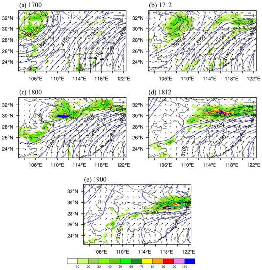
Figure 1.
Geopotential heights (solid blue lines, unit: gpm), wind vectors (unit: m s−1) at 700 hPa, and 12 h accumulated precipitation (shading, unit: mm) at (a) 0000 UTC, 17 June, (b) 1200 UTC, 17 June, (c) 0000 UTC, 18 June, (d) 1200 UTC, 18 June, and (e) 0000 UTC, 19 June 2011.
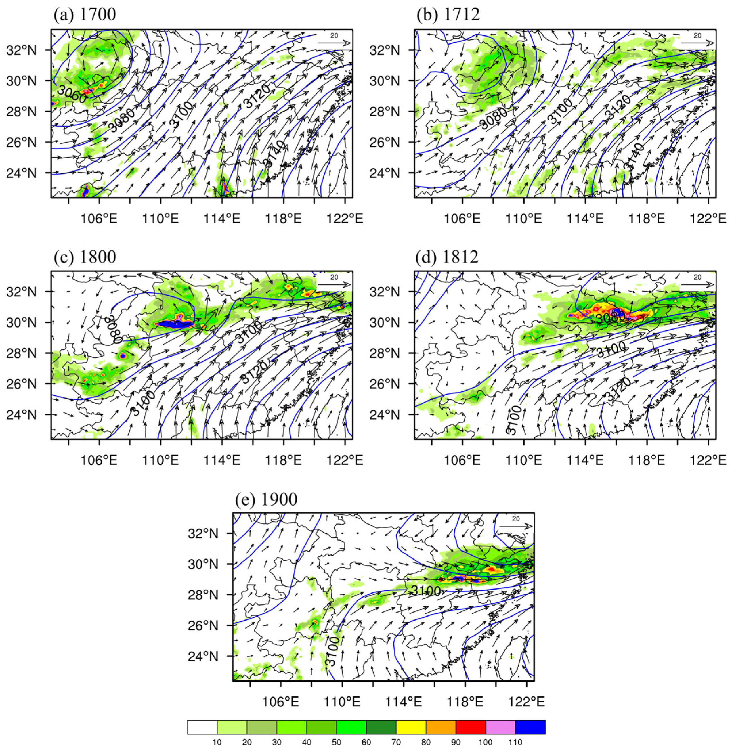
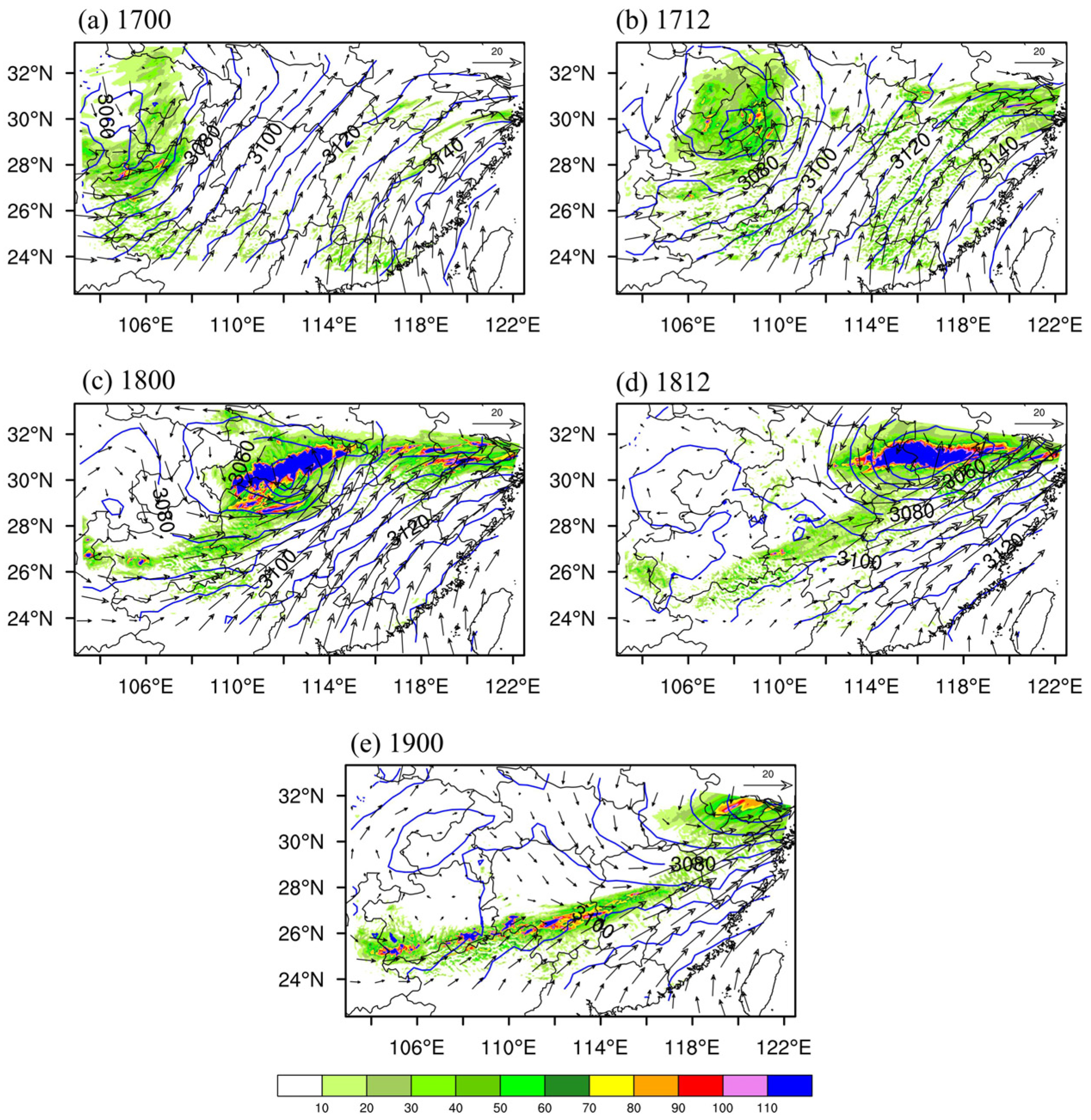
At 0000 UTC, 17 June (Figure 1a), an SWV was generated in the eastern part of the Sichuan Basin with the vortex system centered at . The southeast coast of China was dominated by the Western Pacific subtropical high, and there was a southwesterly wind between the SWV and the subtropical high, with rainfall on the southern and northern sides of the SWV. At 1200 UTC, 17 June (Figure 1b), the SWV moved eastward with the circulation character remaining largely unchanged, and with rainfall occurring in the east of the SWV and banded rainfall appearing to the north of the subtropical high. At 0000 UTC, 18 June (Figure 1c), the SWV continued to move eastward to Hubei Province, with strong wind shear on the eastern side of the SWV and the northern side of the subtropical high. A band of rainfall occurred along the shear line. A northeast–southwest rain belt appeared on the southwestern side of the SWV. At 1200 UTC, 18 June (Figure 1d), the SWV moved to the east of 114 °E, north of the subtropical high, which shifted southward. Strong wind shear formed in the area southward of the SWV and immediately northward of the subtropical high, with a band of rainfall strengthening along the shear line. At 0000 UTC, 19 June (Figure 1e), as the SWV continued to move eastward over the East China Sea, the rainfall on its southern side moved slightly southward, appearing mainly on the southern side of the SWV after 1200 UTC, 18 June. The circulation underwent an adjustment with the eastward movement of the SWV. The shear on the east side of the SWV combined with shear on the northern side of the subtropical high. The pattern of the rainfall also changed from a circular area to a banded distribution.
2.2. Numerical Experiment
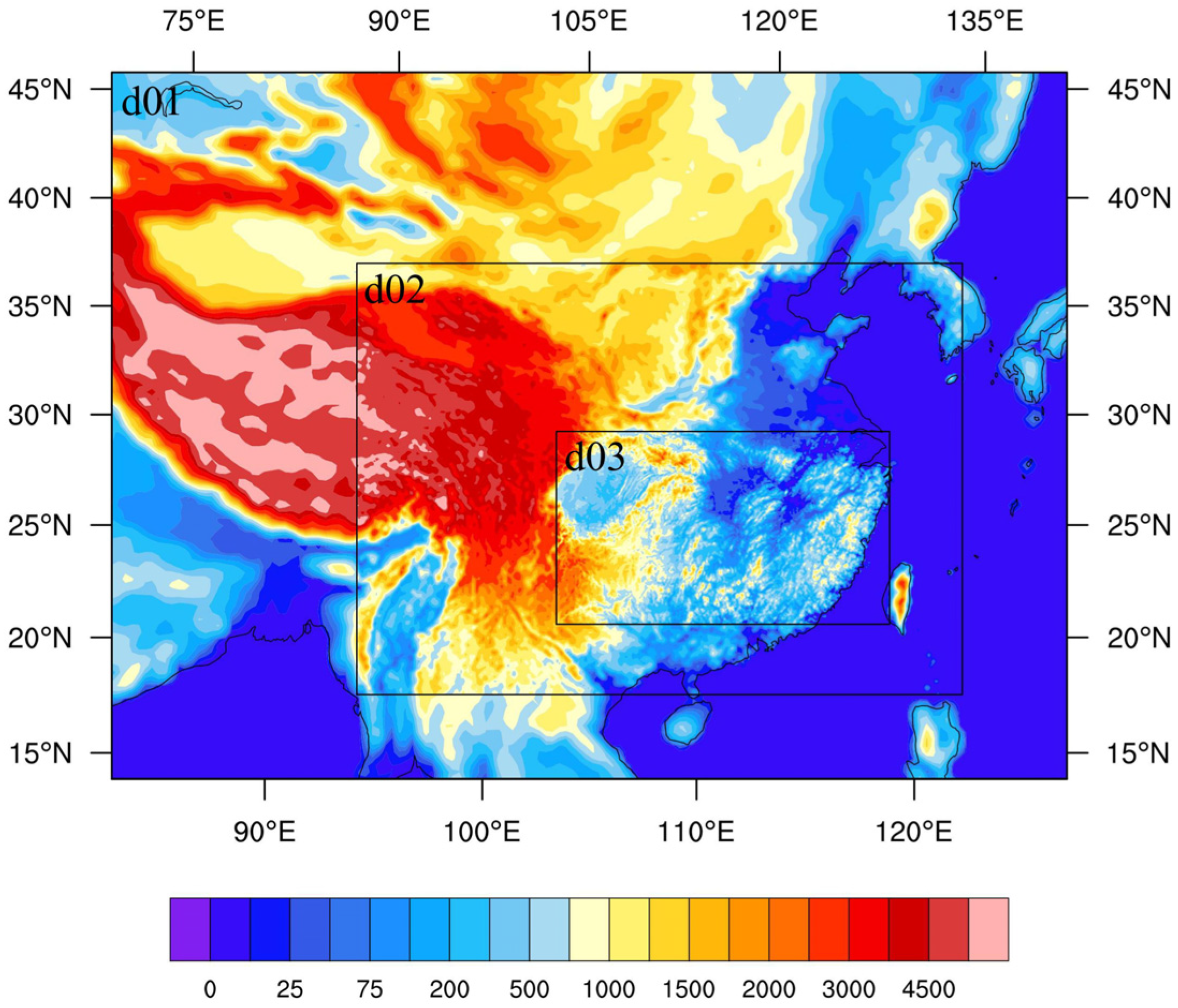
A two-way nested numerical experiment with three domains was performed using the WRF model version 3.6 to simulate the evolution of a SWV. The domains had 30 vertical layers from the surface to 50 hPa, and horizontal grid spacing of 36 km, 12 km, and 4 km with 107 × 144, 195 × 273, and 261 × 450 grid points in horizontal domains, respectively, as shown in Figure 2. Physical parameterization schemes included the Morrison double-moment microphysics scheme, the rapid radiative transfer model for general circulation models (RRTM) longwave radiation transfer scheme [29], the Dudhia shortwave-radiation transfer scheme [30], and the Kain–Fritsch cumulus parameterization scheme [31]. Initial and lateral boundary conditions were derived from the NCEP reanalysis dataset with a horizontal grid spacing of 1° × 1°. The model was integrated for 60 h from 1200 UTC, 16 June to 0000 UTC, 19 June, with hourly output in the innermost nested domain. The time steps for the integration of the model from the outer to inner domain were 180 s, 60 s, and 20 s.

Figure 2.
Model domains. Shading denotes the topography (units: m).
Figure 3 shows simulation results for the geopotential-height field, wind field at 700 hPa, and 12 h accumulated precipitation per 12 h from 0000 UTC, 17 June to 0000 UTC, 19 June in the innermost nested domain. The simulation of the SWV, subtropical high, and precipitation are fundamentally consistent with the actual situation (Figure 1), although with slightly heavier precipitation. In terms of precipitation range and vortex structure, the SWV scale is ~300 km.
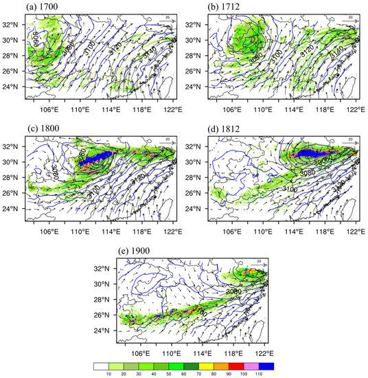
Figure 3.
As in Figure 1, except for the geopotential heights (solid blue lines, unit: gpm), wind vectors (unit: m s−1) at 700 hPa, and 12 h accumulated precipitation (shading, unit: mm) of the WRF model output at (a) 0000 UTC, 17 June, (b) 1200 UTC, 17 June, (c) 0000 UTC, 18 June, (d) 1200 UTC, 18 June, and (e) 0000 UTC, 19 June 2011.
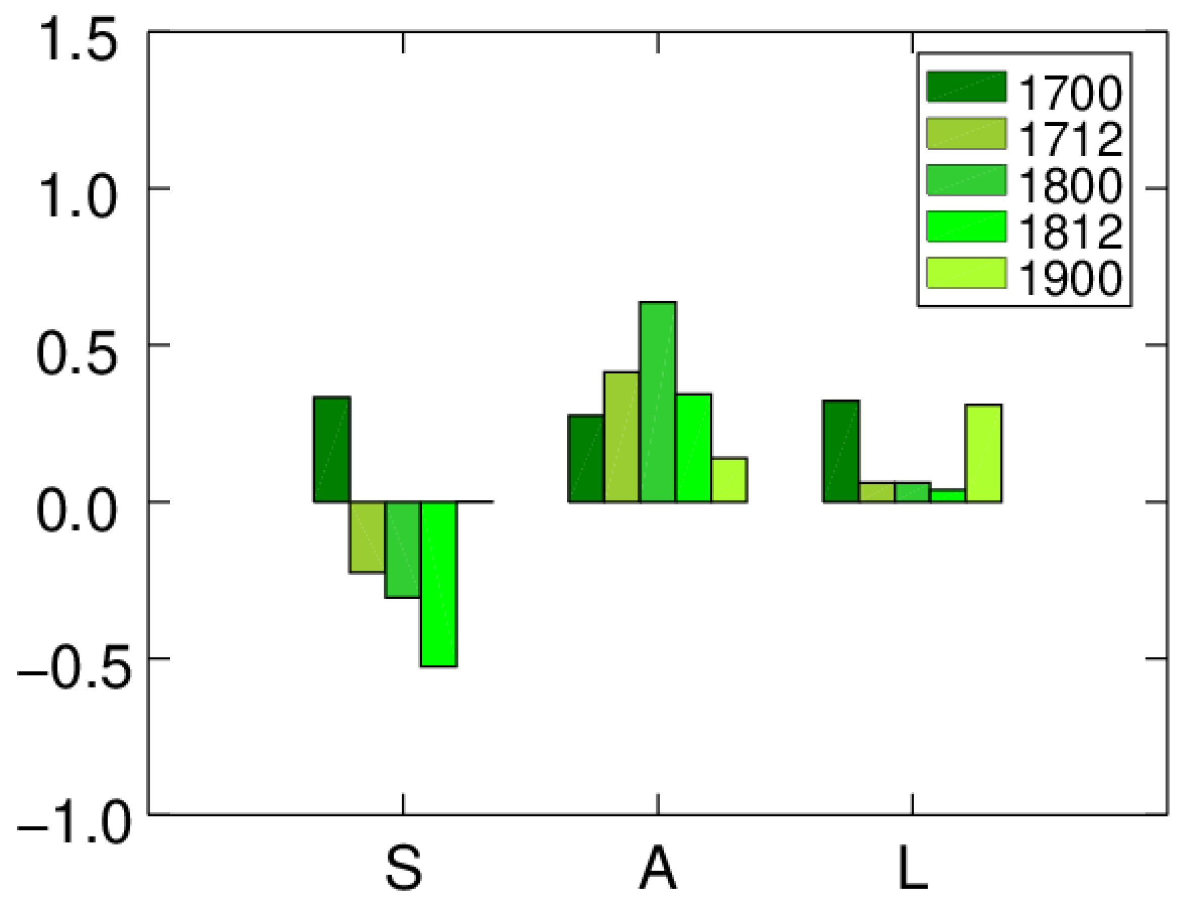
Using the quantitative verification method considering aspects of the structure, amplitude, and location of precipitation forecast (SAL) [32], the 12 h accumulated precipitation per 12 h from 0000 UTC, 17 June to 0000 UTC, 19 June was verified (Figure 4). For the SAL evaluation method, the value L has the most important indicative function, with lower values of L often indicating higher probability of accurate rain prediction; the value A is secondary, and the value S has relatively little indicative function. The values of L from 0000 UTC, 17 June, to 0000 UTC, 19 June, are <0.5, while those at 1200 UTC, 17 June; 0000 UTC, 18 June; and 1200 UTC, 18 June, are ~0.1, indicating that the simulation results reflect the location of the observed precipitation accurately. Values of A from 0000 UTC, 17 June, to 0000 UTC, 19 June, are positive and <0.6, implying that the simulated precipitation is somewhat stronger than that observed. The value of S at 0000 UTC, 17 June, is positive, while being negative at other times, with absolute values of <0.5. Overall, the SAL scores indicate that the distribution and intensity of the simulated precipitation are in good agreement with observations.

Figure 4.
The score of 12 h accumulated precipitation from 0000 UTC, 17 June, to 0000 UTC, 19 June.
The simulation results are thus sufficiently credible for use in analyzing the characteristics of the HKE spectrum during eastward movement of the SWV. Based on variations in circulation and precipitation, the evolution of the SWV can be divided into three stages: the development stage from 1200 UTC, 16 June, to 1200 UTC, 17 June; the mature stage from 1200 UTC, 17 June, to 0600 UTC, 18 June; and the decay stage from 0600 UTC, 18 June, to 0000 UTC, 19 June.
3. Analysis of Horizontal Kinetic Energy Spectra
3.1. The Mathematical Expressions for Horizontal Kinetic Energy
HKE spectra were computed using the two-dimensional discrete cosine transform (DCT) of horizontal velocity at each vertical height level [24,33]. Let and be the DCT of field and , respectively, where is the horizontal wave vector. The HKE spectrum at a given time and vertical level is then
where the dependence on and is suppressed for clarity.
The total horizontal wavenumber is defined as
Spectra were constructed as a function of by angular averaging over wavenumber bands on the plane, with being the central radius of the bands [20]:
where , N = min (Ni, Nj), Ni is the number of zonal grid points, and Nj is the number of meridional grid points. is the wavelength.
3.2. Evolutions of Horizontal Kinetic Energy Spectra
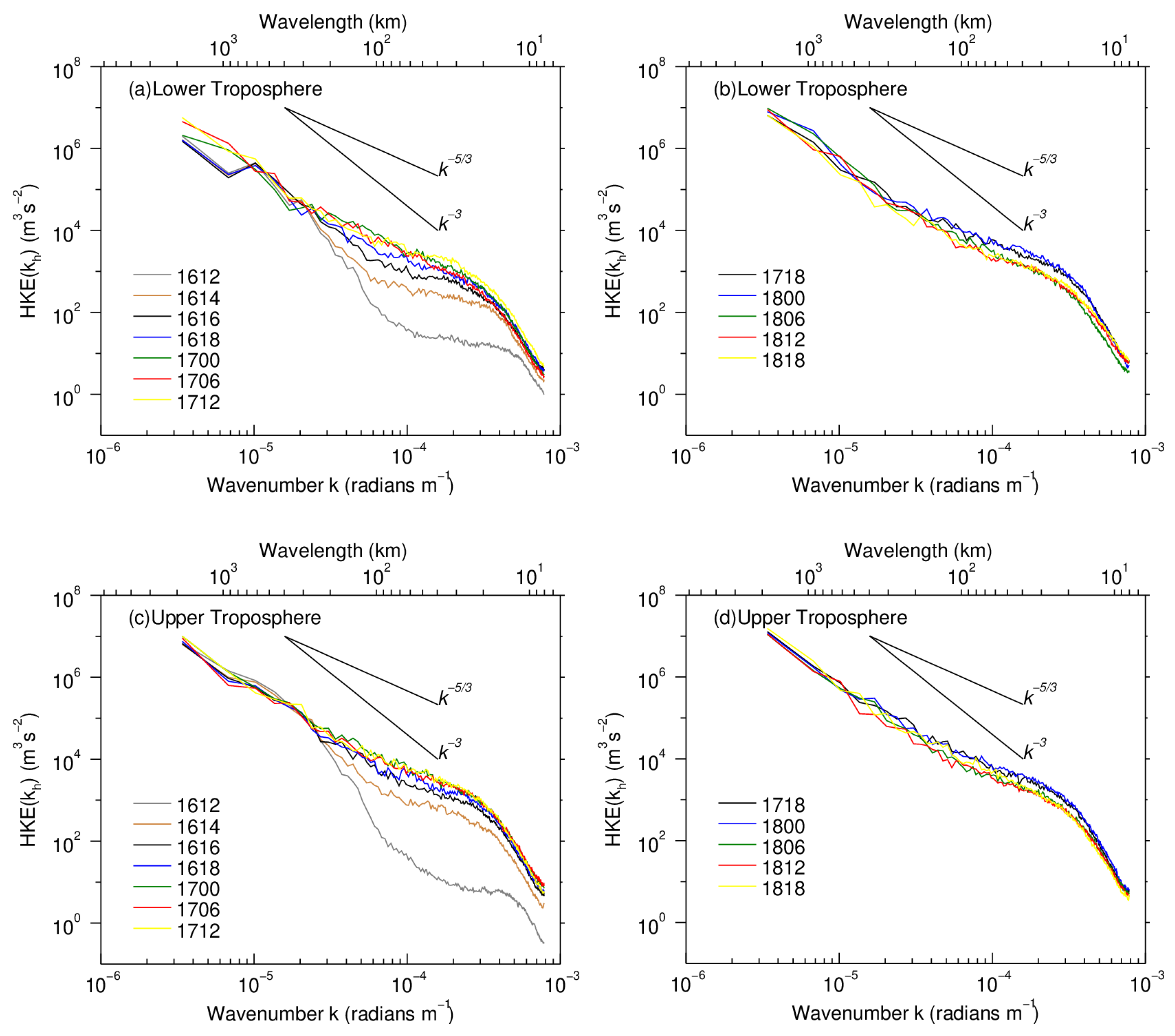
Figure 5 shows the time evolutions of the HKE spectra from 1200 UTC, 16 June, to 1800 UTC, 18 June, in the lower troposphere ( = 5 km), upper troposphere ( = 12 km), and lower stratosphere ( = 20 km), respectively. Because the dissipation term in the WRF model uses the explicit sixth-order diffusion scheme, perturbations smaller than seven times the horizontal grid distance are poorly resolved and are considered unreliable [19]. For data with a horizontal resolution of 4 km, the spectra fall off rapidly for , corresponding to wavelengths of <30 km. Therefore, we focus on the well-resolved horizontal wavelengths of >30 km.

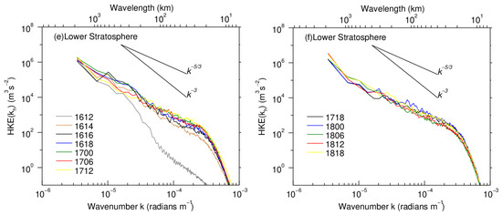
Figure 5.
Horizontal kinetic energy (HKE) spectra from 1200 UTC, 16 June, to 1800 UTC, 18 June, in the (a,b) lower troposphere ( = 5 km), (c,d) upper troposphere (12 km), and (e,f) lower stratosphere (20 km). Spectra were plotted every 2 h until 1800 UTC, 18 June (corresponding to gray, brown, and black lines in the left column, respectively), and every 6 h thereafter. Spectra in the left column pertain to the development stage of the SWV; and those in the right column to the mature and decay stages, with black and blue lines representing spectra from 1800 UTC, 17 June, to 0000 UTC, 18 June (mature stage); and green, red, and yellow lines spectra from 0600 UTC, 18 June, to 1800 UTC, 18 June (decay stage). Reference lines correspond to −3 and −5/3 slopes.
Overall, HKE decreases rapidly with increasing wavenumber at different times and heights, but there are also differences between spectra. During the development stage, the initial HKE spectra at 1200 UTC, 16 June (gray lines in left column, Figure 5), drop sharply at all heights because of model spin-up. The HKE spectra then grow rapidly in the mesoscale range for at each height, while spectra for display relatively little variation with time. After 6 h, the spectral shape at each height remains relatively stable. The time required for spin-up adjustment varies with height, from about 6 h in the lower troposphere (Figure 5a) to 4 h in the upper troposphere (Figure 5c) and only 2 h in the lower stratosphere (Figure 5e). This indicates that the greater the height, the shorter the spin-up time. The evolution of the HKE spectrum at three heights is analyzed below.
During the development stage in the lower troposphere (Figure 5a), the HKE spectra (gray, brown, black, and blue lines in Figure 5a) show a distinct peak at (), indicating initial energy injection at this scale. After 0000 UTC, 17 June (green line in Figure 5a), the peak disappears and HKE increases on both sides at . This suggests that the energy injected at this scale may be consumed through upscale or downscale. After 6 h, the HKE spectrum has already successfully reproduced the −3 slope for () and the −5/3 slope for (). The scale of the spectral transition is approximately 300 km, comparable with the scale of the SWV. This is consistent with the results of Wang et al. [26], in which the scale of the spectral transition also corresponded to that of the TC being simulated. With intensification of the SWV and precipitation, HKE develops on various scales, with growth at the mesoscale for being more significant. HKE at 1200 UTC, 17 June (yellow line in Figure 5a), has much higher values for (). During the mature stage, HKE increases at the mesoscale, with HKE spectra converging over all scales (Figure 5b) and with spectral shape displaying a transition at , where the slope is about −5/3 for and −2.1 for . This indicates that the HKE spectrum falls off more slowly with increasing wavenumber at larger scales. In this stage, HKE (black and blue lines in Figure 5b) for is higher than that at other times. During the decay stage (after 0600 UTC, 18 June), HKE (green, red, and yellow lines in Figure 5b) decreases at all scales, especially at the mesoscale for , distinctly below that at 0000 UTC, 18 June, and 1800 UTC, 17 June (blue and black lines in Figure 5b, respectively). This indicates that the evolution of the HKE spectrum in the lower troposphere is closely related to the development of the SWV.
Compared with the lower troposphere, the spectral slope also changes in the upper troposphere. Although the spectral transition of the HKE spectrum is slightly unclear (Figure 5c,d), the spectral transition still occurs near . The spectral slope is close to −5/3 for and −3 for , similar to spectral characteristics in the lower troposphere. During the mature stage (Figure 5d), the HKE spectra more or less coincide for all scales. The HKE at 1800 UTC, 17 June, and 0000 UTC, 18 June (black and blue lines in Figure 5d, respectively), have higher values for . In the decay stage (Figure 5d), the HKE spectrum (green, red, and yellow lines in Figure 5d) for is lower than that in the mature stage, consistent with its distribution in the lower troposphere (Figure 5b).
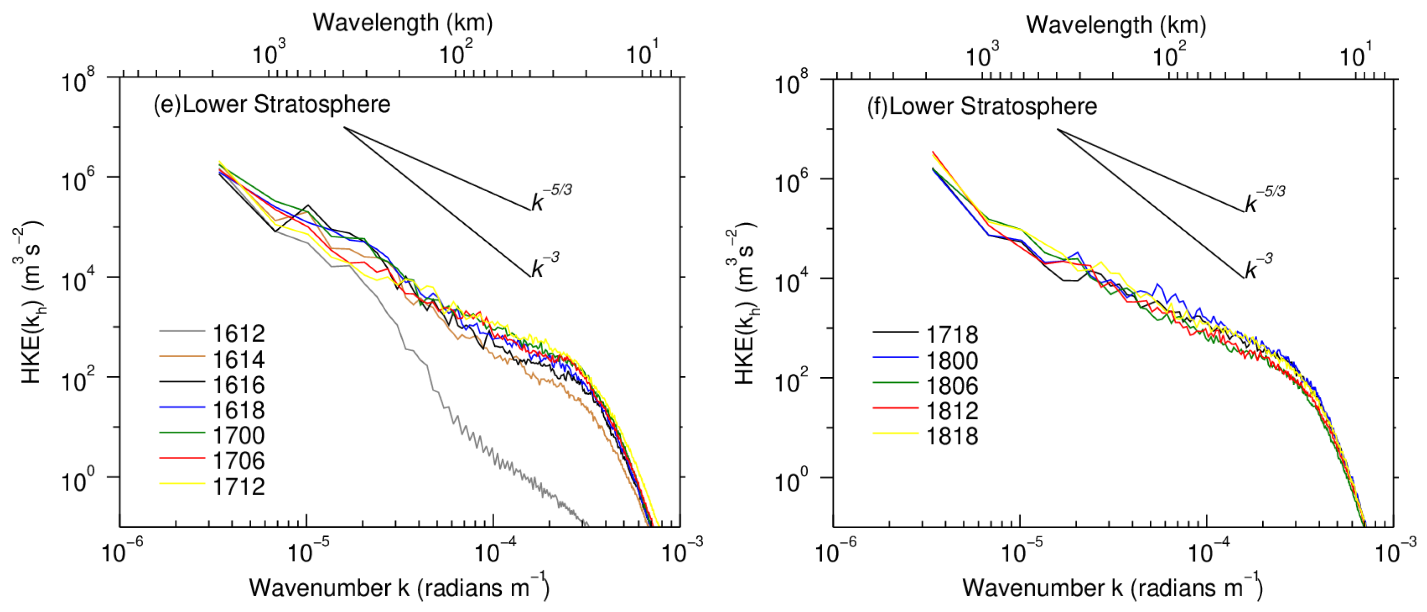
In the lower stratosphere (Figure 5e,f), the HKE spectra at 1400 UTC and 1600 UTC, 16 June (brown and black lines in Figure 5e), also have peaks at , similar to HKE spectra in the lower troposphere (Figure 5a). Compared with those in the troposphere, changes of HKE spectra in the lower stratosphere become more obvious with time, indicating that the intensity of the SWV has a greater influence on the stratospheric HKE spectrum. During the development stage, the HKE spectrum has no clear transition and approaches a quasi −5/3 slope for ; while with intensification of the SWV, the HKE spectrum gradually swells near . This is similar to the HKE spectra of TC in the lower stratosphere [34], where the swell is at (corresponding to the cyclone scale). During the mature and decay stages (Figure 5f), the spectral shape still has a −5/3 slope for , and the HKE spectra at 0000 UTC and 0600 UTC, 18 June (blue and green lines in Figure 5f), have peaks at . For , the HKE at 0000 UTC, 18 June (blue line in Figure 5f), is notably higher than at other times. Furthermore, with the intensification (decay) of the SWV, the HKE in the lower stratosphere for tends to increase (decrease), while that for decreases (increases). This may be due to the presence of an energy injection at and the energy cascade between larger and smaller scales. However, the spectral shapes in Wang et al. [26] and Zheng et al. [34] remain relatively stable and flat throughout the intensification of TC. Differences in HKE spectra in the lower stratosphere between the SWV and TC may be caused by differences in system structure and background circulation.
3.3. Rotational and Divergent Kinetic Energy Spectra
The processes of convergence and divergence, which play key roles in rainstorm development, are important signals of gravity wave activity. Decomposing the HKE spectrum into DKE and RKE spectra is a common method of elucidating the formation of HKE spectra [35]. This decomposition clearly shows the contributions of equilibrium flow and inertial gravity waves to the HKE spectrum [20]. The RKE and DKE spectra can be expressed as follows:
where is the vertical vorticity and is the horizontal divergence. The horizontal wavenumber spectra and are defined analogously to .
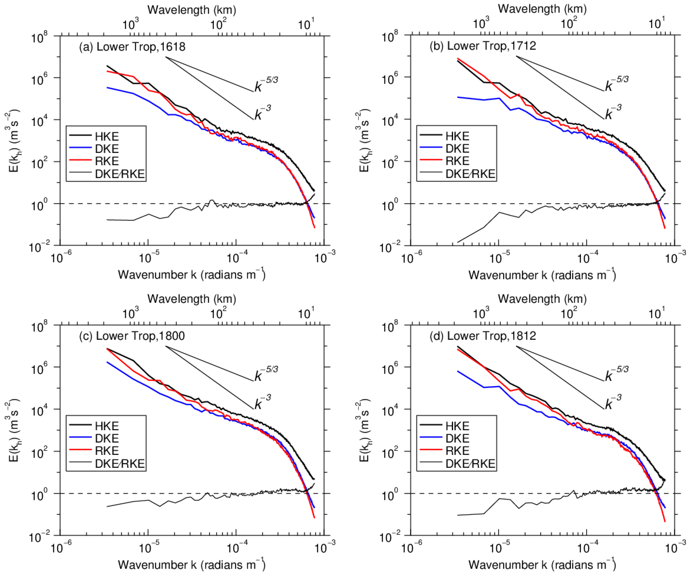
Figure 6 shows HKE, RKE, and DKE spectra and the DKE/RKE ratio averaged vertically over the lower troposphere during different SWV stages. In each stage, the magnitude of RKE is much greater than that of DKE for , while for , the RKE and DKE have the same order of magnitude. The DKE/RKE ratio increases as the wavelength decreases. The RKE spectrum develops a slope of approximately −3 for and −5/3 for , with a spectral transition at around 300 km. The DKE spectrum has no apparent spectral transition and develops a −5/3 slope over the whole mesoscale for . It is clear that in the lower troposphere, the total HKE spectrum is dominated by the RKE spectrum for ; while the RKE spectrum declines to almost the same extent as the DKE spectrum for , accounting for the −5/3 slope of the total HKE spectrum. This is consistent with the fact that the SWV is dominated by rotational motion in the lower troposphere and is similar to the results of Waite et al. [21] and Wang et al. [26].
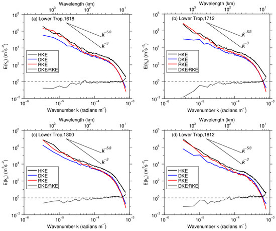
Figure 6.
Horizontal wavenumber spectra of HKE (thick black line), rotational kinetic energy (RKE, thick red line), and divergent kinetic energy (DKE, thick blue line), averaged vertically over the lower troposphere at (a) 1800 UTC, 16 June, (b) 1200 UTC, 17 June, (c) 0000 UTC, 18 June, and (d) 1200 UTC, 18 June. The DKE/RKE ratio (thin black line) is also plotted. Reference lines correspond to −3 and −5/3 slopes.
During the mature stage (Figure 6b,c), the DKE and RKE spectra grow at the same time, with the former gradually approaching the RKE spectrum for , although the magnitude of RKE is still greater than that of DKE. This indicates that as the SWV grows, the divergent motion in the lower troposphere strengthens with the generation of convective precipitation. During the decay stage (Figure 6d), the DKE spectrum drops over all scales; the RKE spectrum has no apparent variations at scales of but falls off at smaller scales (). The magnitude of DKE is thus slightly greater than that of RKE at smaller scales (), indicating that the SWV intensity has an important influence on the DKE spectrum over all scales, and on the RKE spectrum at smaller scales.
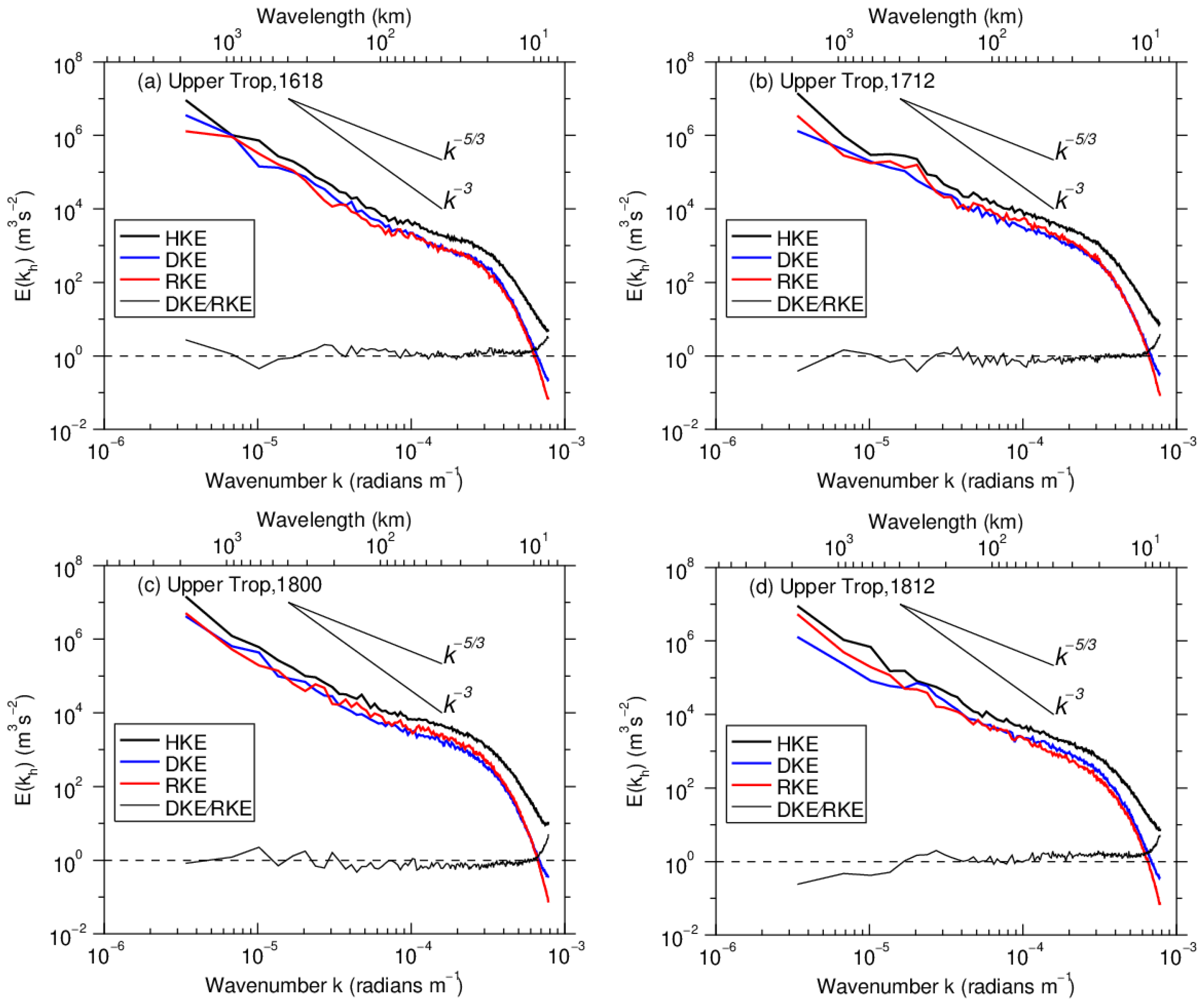
In the upper troposphere (Figure 7), during different stages of the SWV, the RKE and DKE spectra are comparable over all scales, with a ratio of ~1. For , the magnitude of RKE is slightly smaller than that of DKE during the development and decay stages of the SWV (Figure 7a,d); during the mature stage (Figure 7b,c), its magnitude is slightly greater than that of DKE. This demonstrates that the enhancement of the SWV is closely related to enlargement of the RKE spectrum at the mesoscale. Similar to the total HKE spectrum, the RKE and DKE spectra also have spectral transitions. However, with the development of the SWV, the scale of the spectral transition first increases then decreases, from ~100 km at 1800 UTC, 16 June (Figure 7a), to ~300 km at 1200 UTC, 17 June (Figure 7b), and 0000 UTC, 18 June (Figure 7c), before decreasing to 200 km at 1200 UTC, 18 June (Figure 7d).
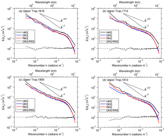
Figure 7.
As in Figure 6, except for the horizontal wavenumber spectra of HKE (thick black line), RKE (thick red line), and DKE (thick blue line), averaged vertically over the upper troposphere at (a) 1800 UTC, 16 June, (b) 1200 UTC, 17 June, (c) 0000 UTC, 18 June, and (d) 1200 UTC, 18 June. The DKE/RKE ratio (thin black line) is also plotted. Reference lines correspond to −3 and −5/3 slopes.
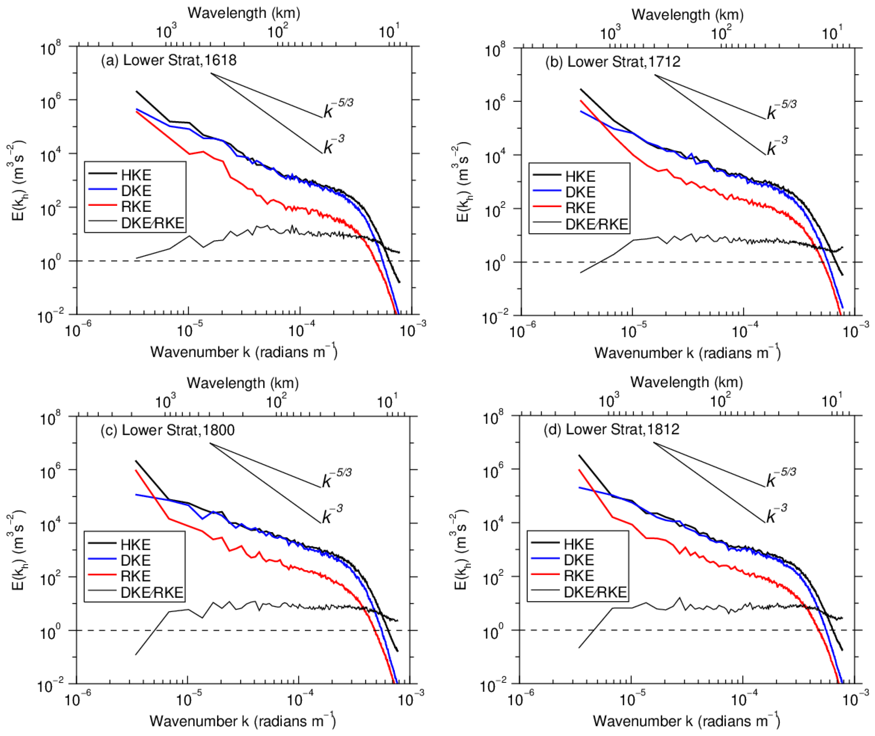
In the lower stratosphere (Figure 8), the RKE and DKE spectra are obviously different from those in the troposphere (Figure 6 and Figure 7). The DKE is almost an order of magnitude larger than the RKE, and the HKE spectrum is largely dominated by the DKE spectrum. This is due to the rotational motion of the SWV, which is significant in the troposphere but does not propagate upward to the stratosphere, with gravity wave activity caused by the SWV being the most important signal in the lower stratospheric atmosphere [36]. This is consistent with the TC simulation, where the DKE spectrum and resultant HKE spectrum in the lower stratosphere have a quasi-linear distribution with a −5/3 slope [26]. Similarly, the DKE and total HKE spectra during different stages of the SWV maintain a slope of −5/3 over the mesoscale range. In contrast to the HKE and DKE spectra, the RKE spectrum changes markedly during three stages. During the development stage, it displays a transition at around with an approximately −3 slope for and a −5/3 slope for . At 1200 UTC, 17 June (Figure 8b), the scale of the RKE spectral transition increases to 300 km, but at 0000 UTC, 18 June (Figure 8c), it has no distinct spectral transition at the mesoscale with a −5/3 slope for . During the decay stage (Figure 8d), the RKE spectrum has a −5/3 slope for and a −2.1 slope for , where is the transition scale. Thus, the evolution of the RKE spectrum in the lower stratosphere suggests that the energy first grows at the mesoscale before cascading upscale.
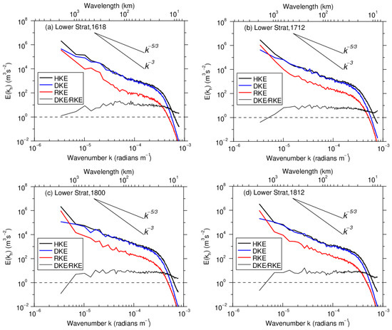
Figure 8.
As in Figure 6, except for the horizontal wavenumber spectra of HKE (thick black line), RKE (thick red line), and DKE (thick blue line), averaged vertically over the lower stratosphere at (a) 1800 UTC, 16 June, (b) 1200 UTC, 17 June, (c) 0000 UTC, 18 June, and (d) 1200 UTC, 18 June. The DKE/RKE ratio (thin black line) is also plotted. Reference lines correspond to −3 and −5/3 slopes.
4. Discussion
The SWV is a cyclonic depression system generated in Sichuan Province, China. An eastward-moving SWV can cause convective precipitation in the middle and lower reaches of the Yangtze River. The TC generated in the western Pacific Ocean which normally moves westward and northward is also a cyclonic depression system. It can induce severe convection and heavy rainfall along the path of TC. Although both are mesoscale vortex systems, their structure and generation mechanism are inevitably different. Therefore, these also cause differences in the distribution and evolution of the HKE spectrum. In the study of Wang et al. [26], the HKE spectrum does not show spectral transition characteristics—not only in the stratosphere but also in the troposphere. It presents a local peak at (i.e., the cyclone scale) and an arc-like distribution at smaller scales in the troposphere, but a quasi-linear −5/3 slope in the lower stratosphere. The HKE spectrum of the SWV in the stratosphere with a slope of −5/3 is similar to that of the TC. However, the HKE spectrum in the troposphere shows a distinct transition. Its transition scale is approximately 300 km, and the HKE spectrum has a slope of approximately −3 for and −5/3 for .
The eastward movement of the SWV to the middle and lower reaches of the Yangtze River tends to combine with the Meiyu front, which enhances the precipitation of the Meiyu front system. Comparing the HKE spectrum of the SWV with that of the Meiyu front system [24], it is found that in the mature stage of the Meiyu front system, the HKE spectrum in the upper troposphere shows clear transition: the slope of the HKE spectrum is about −3 for , and becomes flat to −5/3 over smaller scales for . In the lower stratosphere, the HKE spectrum also shows a clear spectral transition. For the Meiyu front system, there is a spectral transition scale of around 400 km in both the upper troposphere and the lower stratosphere, and this scale is slightly larger than that of the SWV. For the SWV system, the spectral transition appears not only in the lower troposphere but also in the upper troposphere; however, in the lower stratosphere, the phenomenon of spectral transition is not obvious.
In the study of Peng et al. [24], the relative contribution of DKE and RKE to the total HKE spectrum in the Meiyu front system was also investigated. They found that the DKE was slightly smaller than the RKE in the upper troposphere, and slightly larger than the RKE in the lower stratosphere. For the SWV system, the magnitudes of DKE and RKE in the upper troposphere are also comparable. However, in the lower stratosphere, the DKE has much greater values than the RKE. This is significantly different from that of the Meiyu front system [24] and may be attributed to diverse structures of weather systems. Note that in the Meiyu front system of Peng et al. [24], they referred to = 12–15 km as the lower stratosphere (Figure 10b in Peng et al. [24]). However, the DKE in the lower stratosphere is investigated over = 18–20 km in our study and the upward propagating gravity waves can be prominently found above = 15 km (Figure 4d in Yu et al. [37]). In addition, the background winds play the key role in filtering the wave spectrum [36]. Most of the upward propagating gravity waves are filtered by the background wind. Due to different background conditions in the Meiyu front and the SWV system, the upward propagating gravity waves are affected in various degrees. Therefore, the DKE shows different characteristics in different weather systems.
The comparative analyses show that the distribution and variation of the HKE spectrum have a strong relationship with the weather system. The characteristics of the HKE spectrum in different weather systems have both similarities and distinct differences. Therefore, it is necessary to investigate the characteristics of the HKE spectrum in an eastward-moving SWV system.
5. Conclusions
The WRF model is used to simulate an SWV moving eastward from Sichuan Province, China, during 16–19 June 2011. The WRF simulation reproduces the evolution of the SWV and accompanying precipitation. The SWV process can be divided into the development, mature, and decay stages. Based on the high-resolution simulation, the characteristics of HKE spectra at different heights were analyzed.
In the troposphere, the HKE spectrum displays a −3 slope for wavelengths greater than 300 km and a −5/3 slope for wavelengths between 300 and 30 km during three stages of the SWV. The transition scale is at a wavelength of 300 km, corresponding to the scale of the SWV. The HKE spectrum for wavelengths between 300 and 30 km is closely related to the intensity of the SWV. Within this scale range, the HKE spectrum develops a shallower slope and grows obviously during the mature stage and declines during the decay stage. This indicates HKE increases or decreases according to the intensity of the SWV during different stages.
However, in the lower stratosphere, the HKE spectrum has no distinct transition and approaches a quasi −5/3 slope for wavelengths between 900 and 30 km. The HKE spectrum in the stratosphere is more sensitive to the intensity of the SWV over all scales and changes more obviously than that in the troposphere. With the intensification of the SWV, the HKE spectrum in the stratosphere gradually swells near a wavelength of 300 km (corresponding to the scale of the SWV). Besides, the HKE for wavelengths less than 300 km tends to increase (decrease), while that for wavelengths greater than 300 km decreases (increases) during the mature (decay) stage. This indicates that the HKE spectrum is flatter and HKE is more energetic during the mature stage of the SWV.
Further investigation of the RKE and DKE spectra reveals that the RKE dominates in the lower troposphere for wavelengths greater than 300 km, reflecting the strong vortical motion of the SWV. The magnitude of the DKE increases with height and the DKE spectrum is comparable with the RKE spectrum in the upper troposphere. Then, in the lower stratosphere, the DKE is almost an order of magnitude larger than the RKE, and the HKE spectrum is dominated by the DKE spectrum, indicating that gravity wave activity is an important phenomenon in the lower stratosphere.
In various weather systems, the distribution and evolution of the HKE spectrum are obviously different due to the differences in the structure, generation mechanism, or the motion mode of each system. This study investigated the characteristics of the HKE spectrum of the SWV and discussed its formation mechanism preliminarily. Diagnostic analysis of HKE spectrum and transformation of energy over different scales will be completed in future studies.
Author Contributions
Conceptualization, S.Y., L.Z. and Y.W.; data curation, J.P.; formal analysis, S.Y., L.Z. and Y.W.; funding acquisition, L.Z. and Y.W.; investigation, J.P.; methodology, S.Y., Y.W. and J.P.; software, S.Y., Y.W. and J.P.; supervision, L.Z. and J.P.; validation, S.Y.; writing–original draft, L.Z. All authors have read and agreed to the published version of the manuscript.
Funding
This research is supported by the National Natural Science Foundation of China, grants 41975066 and 42005053, the Science and Technology Innovation Program of Hunan Province, grant 2021RC3072, and the Research Project of National University of Defense Technology, grant ZK21-46.
Institutional Review Board Statement
Not applicable.
Informed Consent Statement
Not applicable.
Data Availability Statement
The National Centers for Environmental Prediction (NCEP) reanalysis dataset are open for research and available at http://rda.ucar.edu/datasets/ds083.2 (accessed on 15 April 2022), and the Hourly gridded precipitation dataset from automated station measurements in China and CMORPH (the Climate Prediction Center Morphing Technique) analysis are available at http://data.cma.cn/dataService/index/datacode/SEVP_CLI_CHN_MERGE_CMP_PRE_HOUR_GRID_0.10.html (accessed on 15 April 2022).
Conflicts of Interest
The authors declare no conflict of interest.
References
- Zhang, S.; Li, C.; Bai, Y. Energy Analysis on a Heavy Storm Case in North China Caused by Typhoon No. 9406. Chin. J. Atmos. Sci. 2006, 30, 645–659. [Google Scholar]
- Yu, R.; Zhang, M.; Robert, D.C. Analysis of the atmospheric energy budget: A consistency study of available data sets. J. Geophys. Res. 1999, 104, 9655–9662. [Google Scholar] [CrossRef]
- Zheng, Y.; Jin, Z.; Chen, D. Kinetic energy spectrum analysis in a semi-implicit semi-Lagrangian dynamical framework. Acta Meteorol. Sin. 2008, 66, 143–157. [Google Scholar]
- Bierdel, L.; Friederichs, P.; Bentzien, S. Spatial kinetic energy spectra in the convection-permitting limited-area NWP model COSMO-DE. Meteorol. Z. 2012, 21, 245–258. [Google Scholar] [CrossRef]
- Larsen, M.F.; Kelly, M.C.; Gage, K.S. Turbulence spectra in the upper troposphere and lower stratosphere between 2 hours and 40 days. J. Atmos. Sci. 1982, 39, 1035–1041. [Google Scholar]
- Wang, Q.; Tan, Z. Multi-scale topographic control of southwest vortex formation in Tibetan Plateau region in an idealized simulation. J. Geophys. Res. Atmos. 2014, 119, 11543–11561. [Google Scholar] [CrossRef]
- Nastrom, G.D.; Gage, K.S. A Climatology of Atmospheric Wavenumber Spectra of Wind and Temperature Observed by Commercial Aircraft. J. Atmos. Sci. 1985, 42, 950–960. [Google Scholar] [CrossRef] [Green Version]
- Cho, J.Y.N.; Lindborg, E. Horizontal velocity structure functions in the upper troposphere and lower stratosphere: 1. Observations. J. Geophys. Res. Atmos. 2001, 106, 10223–10232. [Google Scholar] [CrossRef]
- Dewan, E.M. Stratospheric wave spectra resembling turbulence. Science 1979, 204, 832–835. [Google Scholar] [CrossRef]
- Gage, K.S. Evidence for a k−5/3 law inertial range in mesoscale two-dimensional turbulence. J. Atmos. Sci. 1979, 36, 1950–1954. [Google Scholar] [CrossRef] [Green Version]
- Tung, K.K.; Orlando, W.W. The k−3 and k−5/3 energy spectrum of atmospheric turbulence: Quasigeostrophic two-level model simulation. J. Atmos. Sci. 2003, 60, 824–835. [Google Scholar] [CrossRef] [Green Version]
- Tulloch, R.; Smith, K.S. Quasigeostrophic Turbulence with Explicit Surface Dynamics: Application to the Atmospheric Energy Spectrum. J. Atmos. Sci. 2009, 66, 450–467. [Google Scholar] [CrossRef]
- Lindborg, E. The energy cascade in a strongly stratified fluid. J. Fluid Mech. 2006, 550, 207–242. [Google Scholar] [CrossRef]
- Kolmogorov, A.N. The local structure of turbulence in incompressible viscous fluid for very large Reynolds number. Dokl. Akad. Nauk SSSR 1941, 30, 301–305. [Google Scholar]
- Koch, S.E.; Jamison, D.B.; Lu, C.; Smith, T.L.; Tollerud, E.I.; Girz, C.; Wang, N.; Lane, T.P.; Shapiro, M.A.; Parrish, D.D.; et al. Turbulence and gravity waves within an upper-level front. J. Atmos. Sci. 2005, 62, 3885–3908. [Google Scholar] [CrossRef]
- Lu, C.; Koch, S.E. Interaction of upper-tropospheric turbulence and gravity waves as obtained from spectral and structure function analyses. J. Atmos. Sci. 2008, 65, 2676–2690. [Google Scholar] [CrossRef]
- Lilly, D.K. Stratified Turbulence and the Mesoscale Variability of the Atmosphere. J. Atmos. Sci. 1983, 40, 749–761. [Google Scholar] [CrossRef] [Green Version]
- Koshyk, J.N.; Hamilton, K. The horizontal kinetic energy spectrum and spectral budget simulated by a high-resolution troposphere-stratosphere-mesosphere GCM. J. Atmos. Sci. 2001, 58, 329–348. [Google Scholar] [CrossRef] [Green Version]
- Skamarock, W.C. Evaluating Mesoscale NWP Models Using Kinetic Energy Spectra. Mon. Weather Rev. 2004, 132, 3019–3032. [Google Scholar] [CrossRef]
- Waite, M.L.; Snyder, C. The mesoscale kinetic energy spectrum of a baroclinic life cycle. J. Atmos. Sci. 2009, 66, 883–901. [Google Scholar] [CrossRef]
- Waite, M.L.; Snyder, C. Mesoscale energy spectra of moist baroclinic waves. J. Atmos. Sci. 2013, 70, 1242–1256. [Google Scholar] [CrossRef] [Green Version]
- Peng, J.; Zhang, L.; Zhang, Y. On the Local Available Energetics in a Moist Compressible Atmosphere. J. Atmos. Sci. 2015, 72, 1551–1561. [Google Scholar] [CrossRef]
- Peng, J.; Zhang, L.; Guan, J. Applications of a Moist Nonhydrostatic Formulation of the Spectral Energy Budget to Baroclinic Waves. Part II: The Upper-Tropospheric Energy Spectra. J. Atmos. Sci. 2015, 72, 3923–3939. [Google Scholar] [CrossRef]
- Peng, J.; Zhang, L.; Luo, Y.; Zhang, Y. Mesoscale Energy Spectra of the Mei-Yu Front System. Part I: Kinetic Energy Spectra. J. Atmos. Sci. 2014, 71, 37–55. [Google Scholar] [CrossRef]
- Sun, Y.Q.; Rotunno, R.; Zhang, F. Contributions of moist convection and internal gravity waves to building the atmospheric −5/3 kinetic energy spectra. J. Atmos. Sci. 2017, 74, 185–201. [Google Scholar] [CrossRef] [Green Version]
- Wang, Y.; Zhang, L.; Peng, J.; Liu, S. Mesoscale horizontal kinetic energy spectra of a tropical cyclone. J. Atmos. Sci. 2018, 75, 3579–3596. [Google Scholar] [CrossRef]
- Sun, Y.; Zhang, F. Intrinsic versus practical limits of atmospheric predictability and the significance of the butterfly effect. J. Atmos. Sci. 2016, 73, 1419–1438. [Google Scholar] [CrossRef] [Green Version]
- Hamilton, K.; Takahashi, Y.O.; Ohfuchi, W. Mesoscale spectrum of atmospheric motions investigated in a very fine resolution global general circulation model. J. Geophys. Res. Atmos. 2008, 113, D18110. [Google Scholar] [CrossRef]
- Mlawer, E.J.; Taubman, S.J.; Brown, P.D.; Iacono, M.J.; Clough, S.A. Radiative transfer for inhomogeneous atmospheres: RRTM, a validated correlated-k model for the longwave. J. Geophys. Res. Atmos. 1997, 102, 16663–16682. [Google Scholar] [CrossRef] [Green Version]
- Dudhia, J. Numerical study of convection observed during the winter monsoon experiment using a mesoscale two-dimensional model. J. Atmos. Sci. 1989, 46, 3077–3107. [Google Scholar] [CrossRef]
- Kain, J.S.; Fritsch, J.M. A one-dimensional entraining/detraining plume model and its application in convective parameterization. J. Atmos. Sci. 1990, 47, 2784–2802. [Google Scholar] [CrossRef] [Green Version]
- Wernli, H.; Paulat, M.; Hagen, M.; Frei, C. SAL—A novel quality measure for the verification of quantitative precipitation forecasts. Mon. Weather Rev. 2008, 136, 4470–4487. [Google Scholar] [CrossRef] [Green Version]
- Boer, G.J.; Shepherd, T.G. Large-Scale Two-Dimensional Turbulence in the Atmosphere. J. Atmos. Sci. 1982, 40, 164–184. [Google Scholar] [CrossRef] [Green Version]
- Zheng, H.; Zhang, Y.; Wang, Y.; Zhang, L.; Peng, J.; Liu, S.; Li, A. Characteristics of Atmospheric Kinetic Energy Spectra during the Intensification of Typhoon Lekima (2019). Appl. Sci. 2020, 10, 6029. [Google Scholar] [CrossRef]
- Lindborg, E. Horizontal Wavenumber Spectra of Vertical Vorticity and Horizontal Divergence in the Upper Troposphere and Lower Stratosphere. J. Atmos. Sci. 2007, 64, 1017–1025. [Google Scholar] [CrossRef]
- Kim, S.Y.; Chun, H.Y. Stratospheric gravity waves generated by Typhoon Saomai (2006): Numerical modeling in a moving frame following the typhoon. J. Atmos. Sci. 2010, 67, 3617–3636. [Google Scholar] [CrossRef]
- Yu, S.; Zhang, L.; Zhang, M.; Wang, Y. Dynamics of Mechanical Oscillator Mechanism for Stratospheric Gravity Waves Generated by Convection. Atmosphere 2020, 11, 942. [Google Scholar] [CrossRef]
Publisher’s Note: MDPI stays neutral with regard to jurisdictional claims in published maps and institutional affiliations. |
© 2022 by the authors. Licensee MDPI, Basel, Switzerland. This article is an open access article distributed under the terms and conditions of the Creative Commons Attribution (CC BY) license (https://creativecommons.org/licenses/by/4.0/).