Article

Airmass Analysis of Size-Resolved Black Carbon Particles Observed in the Arctic Based on Cluster Analysis

1
Department of Environmental Science, Stockholm University, SE-106 91 Stockholm, Sweden
2
Bolin Centre for Climate Research, SE-106 91 Stockholm, Sweden
*
Author to whom correspondence should be addressed.
Atmosphere 2022, 13(5), 648; https://doi.org/10.3390/atmos13050648
Submission received: 3 March 2022 / Revised: 11 April 2022 / Accepted: 15 April 2022 / Published: 20 April 2022
(This article belongs to the Topic The Arctic Atmosphere: Climate and Weather)

Abstract

:
Here we apply new analysis methods and approaches to existing long-term measurement series that provide additional insights into the atmospheric processes that control black carbon (BC) in the Arctic. Based on clustering size distribution data from Zeppelin Observatory for the years 2002–2010, observations classified as ‘Polluted’ were further investigated based on BC properties. The data were split into two subgroups, and while the microphysical and chemical fingerprints of the two subgroups are very similar, they show larger differences in BC concentration and correlation with the particle size distribution. Therefore, a source–receptor analysis was performed with HYSPLIT 10-days backward trajectories for both subsets. We demonstrate that within this ‘Polluted’ category, the airmasses that contributed to the largest BC signal at the Zeppelin station are not necessarily associated with traditional transport pathways from Eurasia. Instead, the strongest signal is from a region east of the Ural Mountains across the continent to the Kamchatka Peninsula.

1. Introduction

Black carbon (BC) is a multifaceted species that is an important component in our environment because of its strong light-absorbing ability Petzold et al. [1]. As one of the main short-lived climate-forcing agents, BC has a significant effect on the Earth’s radiation budget even though compared to other aerosol types the mass fraction of BC in the atmosphere is rather small [2]. Due to its light-absorbing characteristics, the net radiative effect is predicted to cause a warming effect of the Earth system. However the radiative forcing by BC is fluctuating in time and space and hence associated with large uncertainties [2,3].
In addition to the atmospheric direct radiative effect of BC, once deposited onto snow and glaciers, it decreases the Earth’s surface albedo. The darkening of the surface leads to an increase in surface absorption of short wave radiation. This is especially important in the Arctic [4,5,6]. Earlier studies, i.e., Bond et al. [7] and Novakov and Rosen [8], found black carbon to be second to carbon dioxide in warming the climate and contributing significantly to an accelerated melting of snow and ice in the Arctic and on glaciers.
The Arctic has gone through massive changes during the last decades with record temperatures, a warming rate twice the rate of the global average [4,9,10,11] and a diminishing cryosphere with declining sea ice extent [4] and glaciers [12]. As the climate is further changing, improved understanding of BC-related sources and transport to the Arctic is crucial to assess ongoing and future BC-mediated effects on the Arctic radiative budget. This is especially true for remote locations such as the Zeppelin Observatory on Svalbard.
Although the main sources are far away, local sources of BC exist within the Arctic, such as ship traffic, fuel and biomass burning and gas flaring. Stohl et al. [13] and Schmale et al. [14] suggest that these local sources are not well-studied, and they are likely underestimated and will probably be increasingly important in the near future. The bulk of emission sources contributing to BC in the Arctic, however, exist outside the polar circle, and most BC reach the Arctic region through long-range transport [6,15,16]. In addition, long-range seasonal transport of BC to the Arctic requires more research. For instance, Korhonen et al. [17] came to the conclusion that there is a lack in understanding key factors controlling the magnitude and seasonal variation of equivalent BC (eBC, measured optically following the definition by Petzold et al. [18]) mass concentration when comparing long-term data and numerical transport models for the Arctic spring and summer.
Applying new analysis methods and approaches to existing long-term measurement series can provide additional insights of the atmospheric processes that control eBC in the Arctic. For example, in Tunved et al. [19], a novel method was developed to infer eBC size distribution from continuous, long-term time series of absorption coefficient and particle number size distribution (PNSD) at Zeppelin Observatory. In their study, clustering based on amplitude and shape of the PNSDs was used to classify the individual PNSDs into one of four major categories of aerosol types that were subsequently referred to as Washout, Nucleation, Intermediate and Polluted [19]. For each cluster group, an eBC distribution was inferred from statistical relations based on a combination of 9 years of concurrent PSAP (particle soot absorption photometer) and DMPS (differential mobility particles sizer) observations. The method provided feasible results for three categories. However, the cluster group four, ‘Polluted’, was an exception as it yielded partly unphysical results. As the cluster group four made up around 30% of all observations, further investigation was spurred. One aim of this study is to understand why the statistical method employed in Tunved et al. [19] may have failed for these types of aerosol PNSDs.
Specifically, this works aims to provide new insights and answers regarding defining atmospheric processes governing transport to the receptor site as well as properties relating to the mixing state of the aerosol as measured at the Zeppelin Observatory. Airmass transport will be studied using backward trajectories to investigate how source regions and meteorological characteristics of advected airmasses influence the studied receptor. The focus will be on the most polluted aerosol type, referred to as the ’Polluted’ cluster group (or simply group four [19]), and the study will explore how internal variations of BC and its size distribution within this subgroup of aerosols can be explained with the help of source analysis and processes en route to the receptor site. Here we make use of the additional fingerprints based on BC size distributions within the ‘Polluted’ cluster group to understand the observations with respect to mainly optical properties and airmass origin.

2. Materials and Methods

2.1. Zeppelin Data

In brief, the analysis by Tunved et al. [19] followed these steps: The records of PNSD, absorption coefficient and relative humidity (RH) measured at the Zeppelin Observatory for the study period 2002–2010 were taken from the EBAS database. After screening the data based on data flagging, the three data sets were harmonised such that each validated hourly data point contained simultaneous and valid data from all three instruments (PSAP, humidity measurements and DMPS). PNSD data was further remapped to a uniform common size grid ranging from 20–630 nm, distributed over 31 log-spaced bins with a dlogD p of 0.05. To avoid sampling artefacts, situations where the station potentially could be enveloped by cloud were screened out. As threshold for potential cloudiness, we used RH > 95%. Furthermore, we also removed data collected during the record Arctic smoke event of 2006 (27 April until 4 May [20]). The PNSDs were then clustered into 12 signature distributions which were further grouped according to the shape, amplitude, seasonal and diurnal characteristics as described by Tunved and Ström [19,21]. Based on these characteristics, the 12 signature distributions were converged into 4 groups, each of which can be linked to different atmospheric processes occurring during the history of the airmass transport to the measurement station [19]. The four identified groups are called ‘Washout’ (cluster 1), ‘Nucleation’ (clusters 2–7), ‘Intermediate’ (clusters 8–9) and ‘Polluted’ (clusters 10–12). In the study by Tunved et al. [19], nearly half of the data (43%) were attributed to the ‘Washout’ group, 5.8% to the ‘Nucleation’, 17.4% to the ‘Intermediate’ and about a third (33.4%) to the ‘Polluted’ group (comp. Table A1).
The connected term ‘Polluted’ was corroborated by comparing the chemical signature for the four groups with respect to major ions, sulphate, ammonium and carbon monoxide (CO), which are presented in Figure A2a. For tracers typical of anthropogenic emissions, such as, e.g., sulphate and CO, cluster group 4 presented the highest values and a seasonal variation that is typical for air pollution in the Arctic: a clean summer period, a more polluted wintertime and a maximum during spring, related to the phenomenon of Arctic Haze.
The applied conversion from the bulk absorption coefficient to BC content is based on the correlation between size-dependent particle number concentration and the measured absorption coefficient. A detailed description of the statistical approach can be found in Tunved et al. [19]. The conversion to mass is based on a calculated mean-specific absorption coefficient (MAC) value (9.4 m 2 g 1 ), which was established from the laboratory (see [19]). The resulting inferred BC values produced reasonable results for 3 out of the 4 cluster groups. The group categorised as polluted resulted in an overestimation of BC particles in the Aitken mode, yielding an inferred concentration of eBC particles higher than the total number of particles in this size range (c.f. Figure A4). In consideration of this result, a more in-depth analysis into the ‘Polluted’ group is necessary.

2.2. BC Number Size Distribution

The method in [19] produced for each cluster group a mean dNeBC/dlog D p . This average dNeBC/dlog D p is based on the correlation between the absorption coefficient and the PNSD. With the ratio between shown in Figure A4, dNeBC/dlog D p can be related to the group’s actual dN/dlog D p to yield the fraction of BC particles per bin. Conversely, the average number fraction of eBC particles per size bin can be used to recalculate an approximate absorption coefficient for each individual PNSD for a given particle density ( ρ ) and prescribed MAC:
σ a b s , e s t = 0 M A C N ( D p ) V ( D p ) ρ ( D p ) d D p
where N(D p ) and V(D p ) are the number concentration for particles and volume of a particle of size D p , respectively. As this is the same quantity delivered by the PSAP, the calculation of inferred σ a b s , e s t allows for direct comparison with the true PSAP value, yielding information regarding how well the method performs for each one of the four major cluster groups.
Following the method outlined above, the nature of the ‘Polluted’ group was investigated closer, and the inferred absorption coefficient ( σ a b s , e s t ) was calculated for each observation of PNSD belonging to the group. The derived fraction of BC particles is a function of particle size based on the average observed σ a b s , PSAP for the whole cluster group 4 in relation to the measured PNSD (see Figure A4). The inferred σ a b s , e s t was related to the actual σ a b s , PSAP . The result is presented in Figure 1a. One should at this point take note of the fact that the only parameter that varies in this calculation is the PNSD as observed by the DMPS. Particle density, MAC-value and fraction of BC-particles per bin are constant for the whole group. Hence, this approach assumes that for every size distribution in the ‘Polluted’ group, BC is distributed according to the ratio d N e B C ( D p ) d N ( D p ) as shown in Figure A4.
From Figure 1a, it is clear that the assumption about a common distribution failed as the distribution of the data points are separated into two populations. On the one hand, the method clearly overestimates the observed absorption, and on the other hand, the method substantially underestimates the observed absorption coefficient. The number of observations in the two subgroups are essentially equally separated by the 1:1 line in Figure 1a. Therefore, the data were split into two sets, one above and the other below the 1:1 line. Then, the eBC distribution was recalculated for each one of these subgroups following the statistical approach outlined in Section 2.1. Subsequently, the scaling of the eBC size distribution for the two subsets was recalculated, and the new results are shown in Figure 1b. The amount of data in the two groups is very similar and within 1% (comp. Table A1). The scatter plot of σ a b s , e s t versus σ a b s , PSAP resulting from the two recalculated dNeBC/dlog D p (Figure 1b) show a much better agreement as compared to the case before with one dNeBC/dlog D p for the entire group (comp. Figure 1a).
The resulting eBC distributions for both subgroups can be seen in Figure 2. Although the PNSDs for both subgroups have the same amplitude in the accumulation mode, the eBC distributions differ from each other. Subgroup 1 is characterised by a bimodal shape with a maximum in the Aitken and one in the accumulation mode. In contrast, Subgroup 2 is monomodal with a peak in the Aitken mode. In addition, whereas the median BC distribution in Subgroup 1 makes up a smaller fraction of particles compared to the actual PNSD, the opposite is true for Subgroup 2. In the second subgroup, the dNeBC/dlog D p is clearly overestimating the available particles in the Aitken mode. The division into subgroups as displayed in Figure 1b provides better agreement between measured and calculated absorption coefficients, but it is still evident from Figure 2 that the method is not performing perfectly. This suggests that the statistical approach to derive BC size distributions fails to provide a realistic dNeBC/dlog D p distribution even though the calculated values of the integral absorption σ a b s , e s t is somewhat in agreement with the actual observed σ a b s , P S A P (cf. Figure 1b).
However, the most important insight is that although both subgroups are characterised as polluted based on their microphysical characteristics (comp. Section 2.1 [19]), they are very different with respect to the relationship of BC and particle size distribution, regarding both total absorption and how the equivalent BC is distributed over the studied size range. The reason for the overestimation of BC in the Aitken mode in Subgroup 2 is not yet fully resolved and can potentially be due to some physical properties such as size-dependent MAC, the mixing state of aerosols or wrongly represented size dependence of the density function applied. Another factor to acknowledge is the absence of particles larger than 630 m in the approach to resolve the absorption signal to dNeBC/dlog D p . This is due to the cut-off diameter of the DMPS system at 630 m, while the absorption measurements by the PSAP draw air from a whole air inlet. This can potentially cause absorbing coarse mode particles to bias the correlation analysis, resulting in unrealistic inferred dNeBC/dlog D p distributions as the method tries to account for particle absorption outside of the particle diameter range from the DMPS. Another option is simply that the numerical approach tends to be too sensitive for small particles for some aerosol types or an interrelationship between small particles and BC. The latter means that small particles correlate with BC without necessarily carrying BC in them.
Though this issue of overestimation cannot be resolved, the differences between the two resulting eBC distributions are interesting, which motivates further investigation. As pointed out, both subgroups are characterised as polluted by the clustering method, a classification based on PNSDs properties and their chemical properties, but clearly have very different internal properties with respect to BC. The possibility exists that the difference in eBC magnitude and predicted distribution could be the result of different, yet polluted-type, airmasses arriving at the Zeppelin Observatory. Therefore, in the following section, the two subgroups are used as fingerprints to study potential differences in source contributions.

2.3. Back-Trajectories with HYSPLIT

To identify source regions for each of the cluster groups, ensemble back-trajectories were calculated using HYSPLIT4 version 5.0.0 [22]. The meteorological data the trajectories are based on come from two sources: FNL and GDAS. For the years 2000–2005, the data were provided by FNL, and for the years 2006–2010, data from GDAS were used. A small difference for the datasets is the horizontal grid resolution, the resolution of FNL is 1.7° × 1.7 ° , while GDAS works on a 1° × 1 ° grid. The reason for not using the same meteorological archives is the fact that neither of the two covers the entire time span of this study.
The approach of ensemble trajectories was chosen to retrieve data on the variability of the transport pattern and the source footprint within the model. For each hourly size distribution, a total of 27 ensemble members were calculated. The centre trajectory of the ensemble cast starts above the Zeppelin Station at 78.9° N, 11.9° E and 480 m agl. The other 26 ensemble members are calculated with a slight offset on the horizontal plane and vertical level from the station. The horizontal perturbation was chosen to be one-tenth of the grid box (≈10 km) and vertically approximately 25 m (0.01 sigma unit).

2.4. Trajectory Source Mapping

In the following analysis, all trajectories in the ensemble are treated with equal weight. Each trajectory is checked for completeness of 240 h, with the 10-day mark set to capture BC’s lifetime in the atmosphere IPCC [2]. The individual trajectories were mapped onto a polar stereographic grid projected out from a centre located at the Zeppelin Observatory. The designed grid has a resolution of 0.5° for latitudes between 0–90° and of 2° for the longitudes (−180° to 180°). Next, meteorological and aerosol-related variables are assigned for each grid box and for each individual trajectory, and average conditions over the grid cell are evaluated where applicable. Lastly, the total trajectory passes over each grid box are counted to obtain the number of total passes and record the hours spent in each grid box.
For analysis of the dominant transport path, the transport probability function P i , j was calculated:
P i , j = n i , j N
where n i , j is the number of trajectory hits over grid (i,j), and N is the total number of trajectories in the clustered group. The function provides information on the likelihood a trajectory passes over a certain grid cell (i,j). The source attribution function C i , j (see Equation (3)) was evaluated for several parameters. C i , j represents the average receptor concentration that is observed if transport from grid (i,j) occurs. C i , j is calculated
C i , j = c i , j · n i , j n i , j
where c ( i , j ) represents the concentration connected to the individual trajectories and grid passes, and n ( i , j ) represents the number of hits per grid. A high value of C i , j indicates that, on average, high concentrations are observed at the receptor for the trajectories arriving from the grid cell. All grid cells with less than 5 recorded trajectory passings for 1 of the subgroups were flagged and not used. The threshold was chosen based on the 10th percentile for the polluted cluster group, which is 4 trajectories. All grid cells below the threshold where set to NaN-values for all parameters in the analysis, except the accumulated precipitation. The accumulated precipitation represents the total amount of precipitation along the entire trajectory.
Locating the main differences of the two subgroups (see Section 2.2) in term of transport pattern, the transport probability function was recalculated for all trajectories in the two groups together. This ratio transport function (R) was calculated for each of the subgroups accordingly. The subscripts for the grid cell (i,j) were left out for readability.
R sub = n sub n sub 1 + n sub 2
To evaluate the effective contribution of each source area in the two subgroups, the observations were put into relation to each other. This will bring less weight to grids having few high concentration trajectories compared to the cumulative effect in grids with high probability function. Therefore, high values mean that this particular grid cell has a high probability to contribute to the BC signal for a given sub-cluster and vice versa. Therefore, the source attribution function was weighted with the ratio transport function of the subgroup and then normalised:
S i , j = C · R sub ( C · R sub ) min ( C · R sub ) max ( C · R sub ) min

3. Results

In Figure 3, key transport features for both subgroups in the ’Polluted’ cluster group are presented: the transport probability function, ratio transport function, the accumulated precipitation along the trajectory and the source attribution function for the absorption coefficient. Each row represents one of the subgroups, on the upper row Subgroup 1 and in the lower row Subgroup 2. In the first column, the transport probability map can be seen for the two subgroups. The transport probability functions for all four cluster groups (Washout, Nucleation, Intermediate and Polluted) are shown in Figure A3. For the two subgroups, as can be seen in both Figure 3a,e, airmasses are transported over the Arctic Ocean from the Russian coast to the Zeppelin Observatory. Small differences can be identified around the North Atlantic Ocean, the Greenland shelf and at the Russian coastline in the Severnaya Zemlya Archipelago. Subgroup 1 has a higher likelihood for contributions from the Atlantic Ocean, while Subgroup 2 shows more pronounced hotspots over the Greenland shelf and at the Russian coastline. Additionally, a substantial amount of trajectories are transported over the Eastern European and Siberian land mass (see Figure 3e). Although Figure 3a,e represent airmasses with different aerosol properties, they are in general similar to previous findings using backwards trajectory analyses by Stohl [15] and Eleftheriadis et al. [23] showing airmass transport with a continental influence from Eurasia.
In the second column of Figure 3b,f, the characteristic transport features are enhanced by plotting the fractional contribution from each subgroup in the following denoted R i , j , or ratio transport function. That is, the sum of the two subgroups is always one in a given grid cell as R i , j = P i , j ( subgroup ) / P i , j ( all ) .
This new projection clearly shows how the two subgroups accent preferred regions, where one or the other subgroup dominates. Comparing R i , j for Subgroups 1 and 2, it is clear that Subgroup 1 shows a bigger influence from the Atlantic Ocean, along with an increased contribution from Europe, while Subgroup 2 has its main contributions from airmasses originating from Eastern Europe and Russia. R i , j stretches like a band from the Sea of Okhotsk in the far east westwards past the Lena River, Lake Baikal and the Urals, all the way to Moscow. A smaller hotspot can be found in Northern America. Compared to Subgroup 1, only a very minor fraction of airmass trajectories originate from the Atlantic region.
The accumulated precipitation shown in Figure 3c,g follows the main synoptic storm track pattern. In both cases, the most accumulated precipitation is observed in airmasses over the North Atlantic and Central Europe. Furthermore, a relatively high amount of precipitation can be seen along the coastlines of Greenland and Norway. In Subgroup 1, a hotspot is located at the southeast coast of Greenland. This is a feature commonly observed because of the coastline and its rapid incline of the elevation of the Greenland landmass. Similar precipitation hotspots have been reported, e.g., by Hakuba et al. [24], who demonstrated that this region is of climatological importance with most precipitation of Greenland falling along the eastern coast. For Subgroup 2, the maximum precipitation intensity during transport coincide with the airmasses passing over the North Atlantic. In both cases, a prominent precipitation region is located over Canada, although with higher intensities for Subgroup 2. The fact that Subgroup 1 dominates the transport through the region with the most accumulated precipitation is important as this is likely to affect the physical and chemical properties of the aerosol particles transported within the airmasses.
The last column of Figure 3 shows the source attribution function for the absorption signal observed at the Zeppelin Station relative to the trajectory footprint. Instead of an eBC concentration, the absorption coefficient is shown. These two measures are proportional to each other and linked with the MAC value. Converting the coefficient to a concentration is completed by multiplying with the constant MAC value (see Section 2.1). The corresponding values for the two subgroups differ by an order of magnitude, which was indicated in Figure 2b. Subgroup 1 displays a rather even geographical distribution of the magnitude of C i , j , although higher signals can be seen at the edges of the trajectory footprint exemplified by North America and southern parts of the Eurasian continent. In general, however, the values are low, and no distinct pattern appears apart from lower than average absorption observations in airmasses transported over the Atlantic Ocean. The apparent low variability of the source attribution function could potentially be an artefact of a potential memory effect that can appear during the trajectory analysis and subsequent mapping of C i , j . Such memory effects can occur when strong sources are located up- or downstream of the grid cell (i,j) conjuncting with corresponding small sink strength. Likewise, regions with strong sinks close to the receptor may diminish the visibility of prominent sources downstream from these regions, simply due to the fact that the contributions from these source areas never reach the receptor. Subgroup 2 features more distinct regional patterns. Higher absorption signals are mostly associated with transport over the Eastern sector. Airmasses associated with transport over the North Atlantic Ocean, Greenland and most of the North American continent are associated with significantly lower absorption coefficients compared to Eurasia. The maximum values can be found north of the Black Sea. Thus, although the two subgroups both belong to the polluted category and share similar features in PNSD properties and chemical signature, they are markedly different with respect to integral absorption. In addition, as discussed above, the two subgroups are clearly associated with different transport characteristics and source patterns.
To better understand the contribution by each subgroup to the observed absorption coefficient, the absorption signal was weighted with the fraction of observations for the subgroups compared to the whole polluted cluster group.
The resulting quantity, referred to as normalised effective potential source contribution (S i , j ), provides an estimate of the overall contribution from each grid cell (i,j) as the transport weighted absorption represent P i , j * C i , j . S i , j highlights the most important transport pathways, as both transport function and concentration function are included in the S i , j . Areas with lower C i , j can be associated with high S i , j due to more frequent transport (high P i , j ). In that sense, S i , j provides estimates of the various grid cells’ overall contribution to bulk receptor-observed absorption. Hence, both the frequency of transport from a specific area and the observed absorption coefficient are included in this value.
In Figure 4, S i , j for both subgroups is presented. The distribution of S i , j clearly emphasises the differences in transport of light-absorbing particles in the two subgroups. For Subgroup 1 in Figure 4a, the S i , j is distributed evenly around the Arctic Ocean with generally low values. A few areas are slightly more pronounced over the North Sea, at the coast of Norway and around the Bering Sea. The maximum can be found northwest of the Black Sea; however, the Russian region west of the Urals shows minimal values. For Subgroup 2 (Figure 4b), the main contribution shows a complementing pattern. In contrast to Subgroup 1, high contributions come from the Northern part of Eurasia. The minimum for S i , j in Subgroup 2 can be seen over the North Atlantic and Greenland. At the edge of the trajectories tracking in North America, high contributions can be observed in the Bering Sea for both subgroups.
The two Subgroups can be distinguished from each other by the magnitude of S i , j , which in turn reflects both the transport probability and the grid average concentration. This tells us that although some regions may appear as emission hotspots, the same regions may in fact be of lesser significance as they are associated only with a few transport cases (cf., e.g., Figure 3d and Figure 4a). For Subgroup 1, a concentration hotspot is highlighted in Asia, but S i , j for the same regions is comparably small due to less frequent transport. For Subgroup 2 on the other hand, S i , j (Figure 4b) accentuates the Northern Eurasia region as a potential source region (Figure 3h) with a higher transport probability (Figure 3e).

4. Discussion

Based on the clustering of the PNSDs, the question of how the properties of inferred size distribution for eBC (dNeBC/dlogD p ) may be controlled by source areas and airmass transport characteristics en route to Svalbard was explored. The focus has been on polluted airmasses, mainly observations coinciding with the typical time frame of Arctic Haze. The classification, previously published in Tunved et al. [19], has been based on cluster analysis of PNSDs observed at the Zeppelin Observatory and further corroborated by analysis of major particle-bound ions as well as trace gas concentrations. For these data, characterised as polluted, we have expanded on the methodology presented in Tunved et al. [19] to show that although size distributions within this group are very similar, the associated eBC burden in the group can spread widely. The associated eBC can be used to divide the data into two subgroups which are noticeably different in the estimated size-resolved eBC distribution. Subgroup 1 was found to be associated with a bimodal eBC distribution, peaking in the Aitken and accumulation modes, while Subgroup 2 peaked unimodally in the Aitken mode. This peak in the dNeBC/dlogD p distribution of Subgroup 2 exceeded the total number of particles as given by the PNSD. Besides the differences in inferred eBC, Subgroup 2 is associated with more than four times the BC amount (comparing medians). The nature of the inferred eBC for Subgroup 2 is nontrivial. An exact reason cannot be provide, but the eBC signature highlights the different characteristics of the subgroups. As to why this substantial difference is present, we performed a source receptor analysis to compare the transport characteristics associated with the two subgroups and identified pronounced differences in general transport features.
Backwards trajectories are an established method to analyse atmospheric transport to a receptor site. In several studies, common transport sectors for Arctic BC aerosol were identified. A dominant potential contribution source was Northern Eurasia [25,26] and Central Russia [23]. In this study, we have based the airmass analysis on 10-day back trajectories studied parameters that include transport probability function (P i , j ), source attribution function ( C i , j ), precipitation history and the normalised effective potential source contribution (S i , j ). The latter reflects the combined effect of P i , j and C i , j , and as such, it serves as a representation of the overall importance of different source regions as it takes into account both the potential source strength and transport frequency, respectively.
We have shown, using the S i , j , that for the first subgroup a transport route via the North Atlantic Ocean is of comparably high importance and further indicates the Northern Sea and Romania/Moldova as potentially high-impact source regions. In this aspect, a substantially different picture arises for Subgroup 2. A minimum can be seen over the North Atlantic and Europe, which suggests that this transport path is less important as an Arctic BC contributor pathway for this subgroup. Additionally, these areas are affected by maximum accumulated precipitation values. Thus, the aerosol is more likely scavenged out by rain events. The normalised effective potential source contribution (S i , j ) accentuates the influence of the Russian continent for Subgroup 2. The most important sources lay East of the Ural Mountains across the whole landmass to the Pacific Ocean.
Using carbon isotopes, Winiger et al. [27] found a significant contribution from biomass burning at Arctic stations. In the current study, both subgroups show the largest seasonal contribution of eBC during the Arctic Haze season (March–May) [19]. This is also the beginning of wildfires in the Siberian Taiga. The fires North of 55° N are mainly low-intensity surface fires during the fire season (February–May) [28]. Next to wildfires, there is also cropland burning, a common agricultural management practice, which is used in the same region. One of the main seasons for cropland burning is April to May [29]. The regional and seasonal contributions of the fires agree in time and space with our trajectory analysis (see Figure A5). With an increased likelihood of more wildfires and peak seasons [30], together with the changes in transport pattern to the Arctic due to Arctic surface warming and sea ice decline, as suggested by Cassano et al. [31] and Mewes and Jacobi [32], the importance of BC emissions in Northern Eurasia grows.
The findings presented in the current study are in agreement with a recent study by Stathopoulos et al. [33]. They investigated the transport of BC to the Arctic in correlation with the North Atlantic Oscillation (NAO) and the Scandinavian Pattern (SCAN) during a cold (November–April) and warm (May–October) period. While they did not find a significant difference between the NAO index phases, they determined an increase in BC during the negative SCAN indices. Their cold period coincides with the time frame of our polluted cluster. For higher eBC contributions at the Zeppelin Observatory, Siberia was pointed out as a more influential emission region than Europe. The emissions from Siberia are linked to gas flaring by Stathopoulos et al. [33], but as we show, biomass burning is also active on the same temporal and regional scale and should be taken into account. Although we can not definitely attribute transport patterns to sources or sinks, Subgroup 1 shares patterns with precipitation (sink) and Subgroup 2 with Subgroup areas.
Another recent study by Backman et al. [34] calculated 7-days backwards trajectories for several stations in the Arctic over the years 2012–2014. The individual footprint of absorption for the Zeppelin Observatory shows a strong signal east of the Urals, as we also show for Subgroup 2. The contribution of elevated absorption coefficients for the whole Arctic were linked to emissions over Central Asia, and it was concluded that the Indo-Gangetic Plain is a likely source region for BC ending up in the Arctic. These results could not been reproduced with our 10-days backwards trajectories for the period 2002–2010.

5. Summary & Conclusions

In this study, the aim was to better understand the optical properties and airmass origin of the cluster group characterised “polluted” from a preceding study [19] with help of a footprint analysis. This subset of data was classified as polluted based on the shape and magnitude of the associated PNSD properties. The frequency of occurrence of observations belonging to this group peaks during the period commonly associated with Arctic Haze. The classification of these data as “polluted” was further corroborated by simultaneous observations of the chemical composition of the atmosphere, such as CO, SO 2 and major ions.
For this group, Tunved et al. [19] adopted a statistical correlation approach to infer dNeBC/dlogD p from observed variability of the PNSD and the integral light absorption coefficient σ a b s . In the current study, we expanded on that approach, and found that within the polluted group, it is possible to identify two different subgroups, which, although similar in dN/dlogD p , are markedly different with respect to inferred dNeBC/dlogD p . This difference is present regarding both the shape and magnitude of dNeBC/dlogD p . Subgroup 1 shows a median eBC that is 4–5 times less in magnitude than Subgroup 2. For Subgroup 2, with more eBC present, the correlation with the PNSD resulted in an unrealistic eBC size distribution. Although the exact reason for this is not known, the presence of two distinctly different eBC distributions derived from an otherwise similar set of data clearly highlights the difference between the two subgroups.
The goal of this paper has been to explore the difference between the two subsets of data with the aid of trajectory-based source-receptor analysis. The analysis has revealed significant differences in transport-related parameters associated with the two subsets, of which the main findings are presented in bullet form below:
  • Subgroup 1 is associated with transport from a sector including Western Europe/North Atlantic. Transport in this western sector is typically exposed to more precipitation which may act as an effective sink for aerosol particles. More frequent cloud processing may also change the mixing state/shape and density of BC containing aerosol particles due to both physical and chemical effects associated with repeated cycles of activation/evaporation.
  • Airmass source areas for Subgroup 2 are biased towards Eurasia. The source attribution function shows that peak values in BC observed at the Zeppelin Observatory are associated with transport from Northern Eurasia/Russia, and large differences in source attribution function are present comparing Eastern and Western Hemispheres. The eBC associated with Subgroup 2 is not affected by precipitation on its transport path. This could be a reason for higher eBC concentration compared to Subgroup 1.
  • We have introduced the normalised effective potential source contribution (S i , j ) function that represents the product of the transport probability function and the source attribution function. This quantity, which reflects the apparent importance of different source regions contributing to the bulk of BC observations, is markedly different comparing Subgroups 1 and 2. For Subgroup 2, S i , j is dominated by Russia, covering the bulk of northern Eurasia from the Urals eastward. Subgroup 1 instead has the largest contribution of BC from the Western Hemisphere, and comparably less influence from Eastern Eurasia. The potential source regions for the second subgroup co-locate with known biomass-burning areas.
The findings of this study show that additional analysis of observations classified as polluted or associated with a high BC burden are necessary to present valuable information on potential source region and en-route processes. While the microphysical and chemical fingerprints of the two subgroups are very similar and they both are classified as polluted, the source–receptor analysis shows that there are different source regions at play dominating the airmass transport to the Zeppelin Observatory. We demonstrate that within this category, the airmasses that contribute to the largest eBC signal at the Zeppelin station are not necessarily associated with traditional transport pathways from Eurasian continent. Rather, airmasses contributing a higher eBC burden at the Zeppelin Observatory are linked by the potential effective source contribution to the region east of the Ural Mountains across the continent to the Kamchatka Peninsula.

Author Contributions

R.S.C. and P.T. analysed and visualised the data; R.S.C., P.T. and J.S., all discussed the data; R.S.C. wrote the paper; P.T. and J.S. reviewed/edited the manuscript and provided feedback; J.S. took care of project administration. All authors have read and agreed to the published version of the manuscript.

Funding

The project aims at studying sources and sinks of black carbon particles on the basis of the size distribution with assistance of laboratory studies, field observations and numerical models, i.e., backward trajectory calculations. Project funder is the Swedish Research Council (contract 2017-03758).

Institutional Review Board Statement

Not applicable.

Informed Consent Statement

Not applicable.

Data Availability Statement

The data used in this study are available on the Bolin Centre Database hosted by the Bolin Centre, Stockholm, Sweden [35].

Acknowledgments

The trajectories were calculated by using Hybrid Single-Particle Lagrangian Integrated Trajectory (HYSPLIT) model, available under http://www.ready.noaa.gov/HYSPLIT.php (accessed on 1 March 2022). The meteorological data sets used are provided by the National Weather Services National Centers for Environmental Prediction (NCEP). Data were taken from NCEP FNL data set reachable under ftp://arlftp.arlhq.noaa.gov/pub/archives/fnl/ (accessed on 1 March 2022) and from the Global Data Assimilation System (GDAS, ftp://arlftp.arlhq.noaa.gov/pub/archives/gdas1 (accessed on 1 March 2022)). The data for Zeppelin Observatory (CMPS, absorption, chemical composition) were taken from EBAS database (http://ebas.nilu.no/ (accessed on 1 March 2022), last data revision October 2011). Thanks to Daniel Partridge (University of Exeter) for valuable comments on the material.

Conflicts of Interest

The authors declare no conflict of interest.

Abbreviations

The following abbreviations are used in this manuscript:
BCBlack Carbon
eBCequivalent Black Carbon
PNSD      Particle Number Size Distribution
PSAPParticle Soot Absorption Photometer
DMPSDifferential Mobility Particles Sizer
RHRelative Humidity
HYSPLITHybrid Single Particle Lagrangian Integrated Trajectory
NAONorth Atlantic Oscillation
SCANScandinavian Pattern

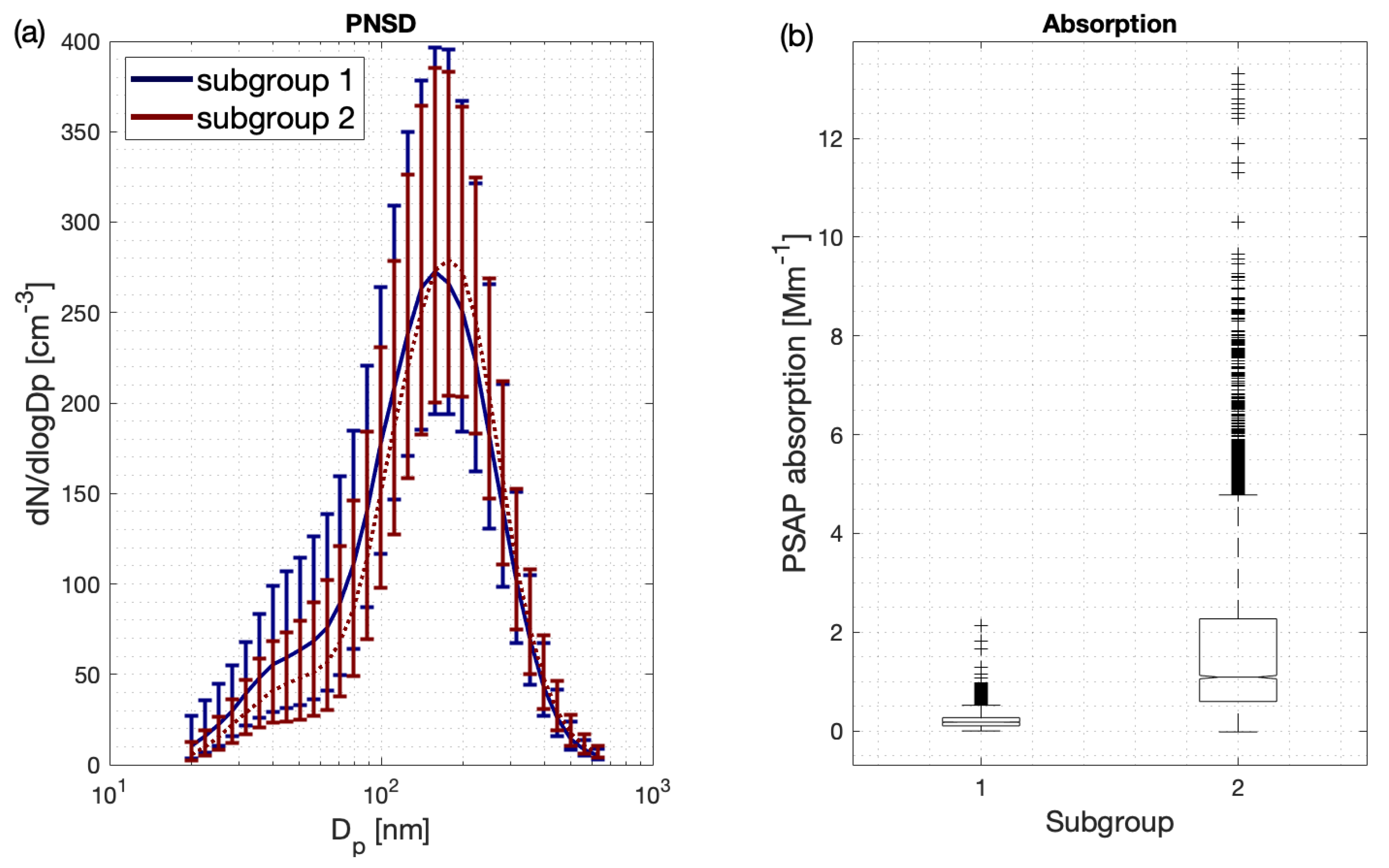
Appendix A. Microphysical Properties

In Figure A1a, the PNSDs for the two subgroups of the polluted cluster is shown. Both PNSDs display a similar shape and amplitude, with a peak in the accumulation mode. There are only small differences in the two subgroups. The second Figure A1b, displays the absorption coefficient measured by the PSAP for both subgroups, displayed as a box plot. It is visible that the absorption coefficient for subgroup 1 is overall very small and does not show a wide spread. The opposite is shown for subgroup 2. The average is higher and the absorption coefficient data show a range of variability.
Figure A1. (a) shows the particle number size distribution in [ cm 3 ] for the two subgroups, Subgroup 1 in blue and Subgroup 2 in red. (b) Absorption in [Mm 1 ] as measured by the PSAP at the station for all valid data points for the two subgroups.
Atmosphere 13 00648 g0a1

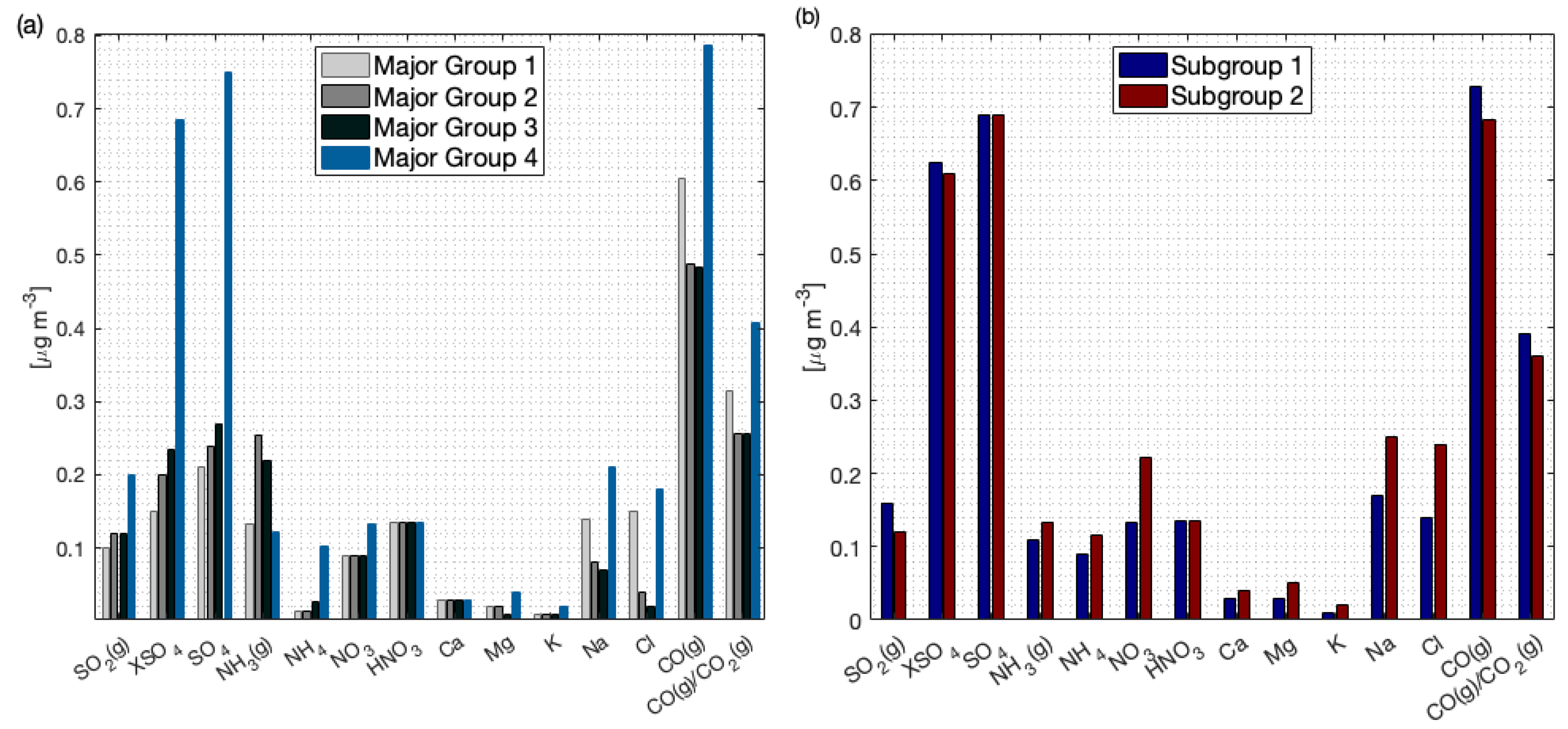
Appendix B. Chemical Composition

Figure A2 shows the median concentration of major species in particle and gas phase for all 4 cluster groups (Figure A2a) and for both subgroups of cluster 4 (Figure A2b). Comparing the polluted cluster group (major group 4) with the other 3 major groups it shows elevated measurements for SO 2 , XSO 4 , SO 4 , NH 4 , NO 3 , Na, Cl, CO(g) and CO(g)/CO 2 (g). The elevated signals corroborate that the airmass measured in major group 4 carries more pollutants than the other cluster groups. In Figure A2b, the same species are shown for the two subgroups of the polluted cluster, but do not attest strong differences in the chemical signature.
Figure A2. Median concentration of major species in particle and gas phase for (a) the four major groups and (b) the two subgroups of major group 4. CO is displayed in units of ppbv/200 and the ratio CO(g)/CO 2 (g) in ppbv/ppmv, all other species in μ gm 3 .
Atmosphere 13 00648 g0a2

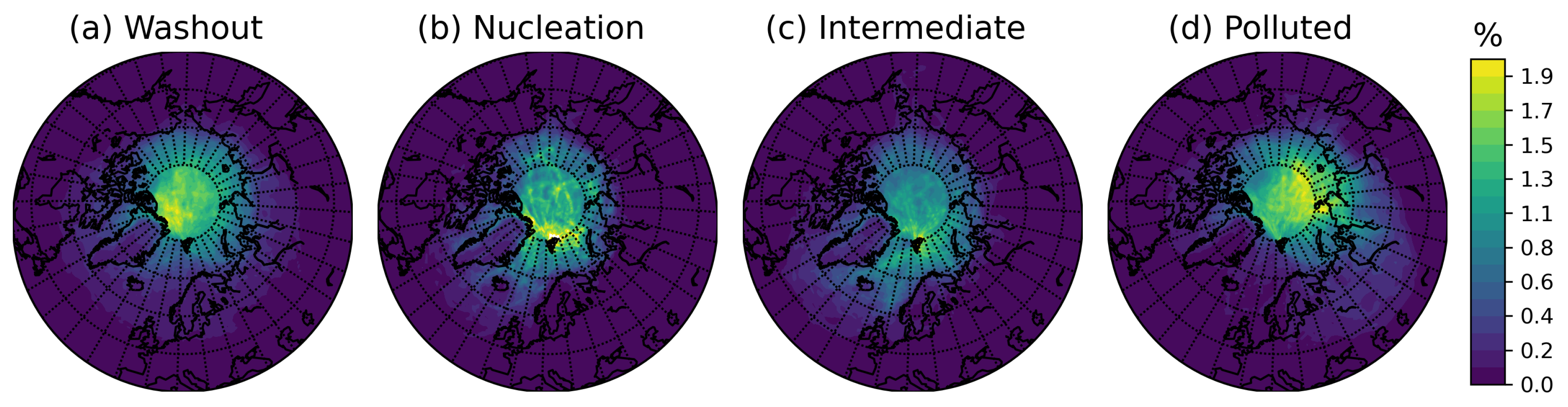
Appendix C. Transport Probability Function

In Figure A3 the most likely travel path for all four cluster groups can be seen. All cover transport from the whole Arctic Ocean and feature small differences. For the largest cluster group, the Washout, most of the airmasses come from the Northern coast of Greenland and travel straight over the Arctic Ocean to the Zeppelin Observatory on Svalbard. The Nucleation group shows a strong influence from the Northern coast of Greenland as well as very high contributions from Svalbard and its immediate surrounding. The extent in distance is shorter and not as uniformly spread. The spreading of the travel pattern could be caused by the smaller amount of observations available for this cluster. The Intermediate clusters shows a tendency from the North Atlantic Ocean and has no clear influence from any land mass. The ‘Polluted’ group displays airmass transport from the east-European and Russian continent.
Figure A3. Transport Probability Map [%] for all four cluster groups: (a) Washout, (b) Nucleation, (c) Intermediate and (d) Polluted.
Atmosphere 13 00648 g0a3
Table A1. Total number of observations and trajectory ensemble runs for each of the clustered groups and the two subgroups.
Cluster GroupWashoutNucleationIntermediatePolluted
TotalSubgroups A & B
# observations14,9011974591711,44756395809
# ensembles14,7291974591511,33256105722

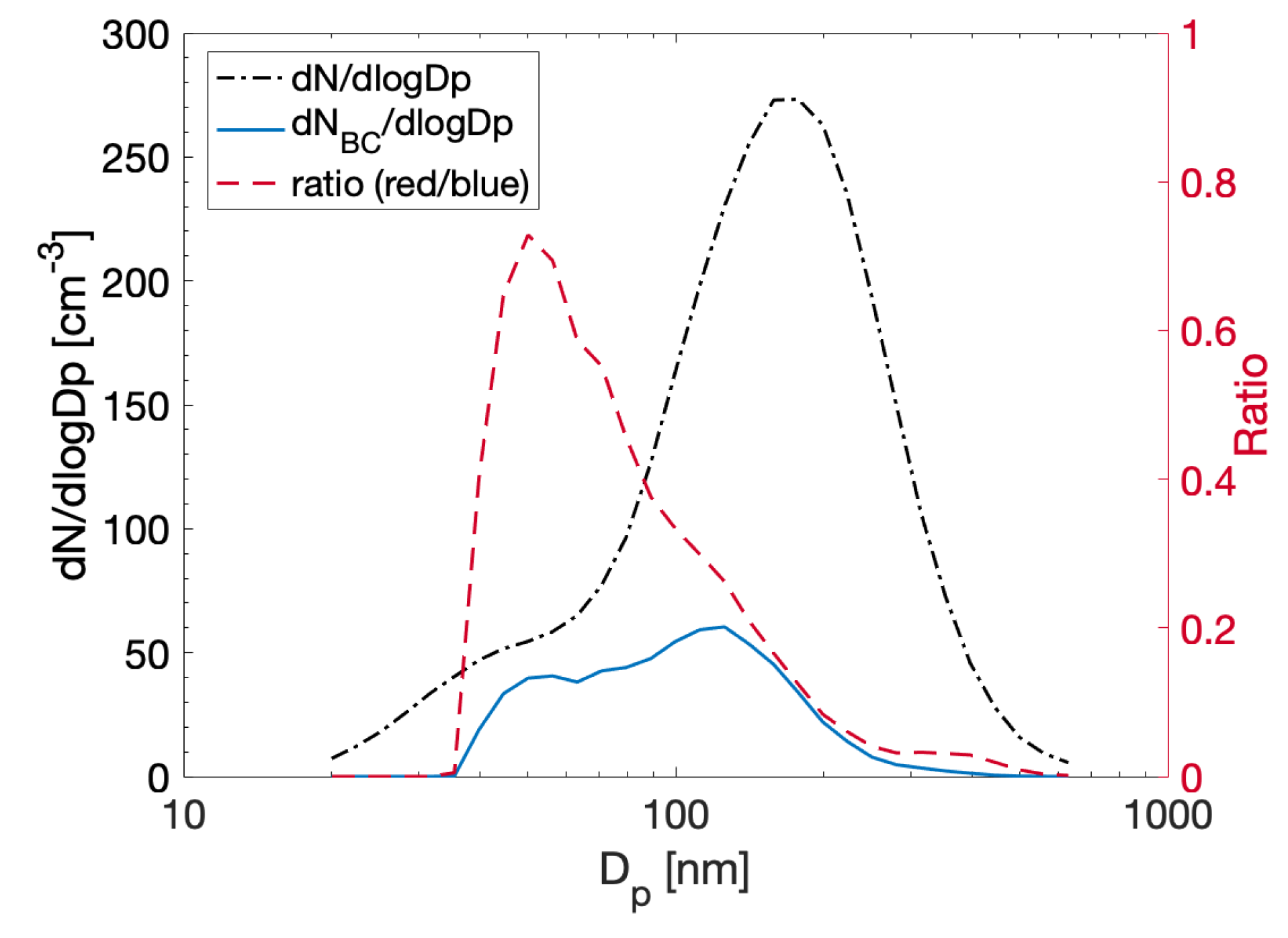
Appendix D. Median Observed Particle Size Distribution

Figure A4 shows the average PNSD of all particles (black) and eBC (blue) for the polluted cluster. The red dashed line shows the ratio between the two number size distributions. The Figure is adapted from [19] to illustrate the statistical approach used and shows how the derived fraction of BC particles is dependent on the particle size and the measured PNSD of all particles.
Figure A4. Adapted from Figure 8 in [19]. Median observed particle size distribution dN / dlogD p (black dash-dotted) and median inferred dN eBC / dlogD p (blue solid) over the particle size. Ratio between the two curves ( dN eBC / dlogD p / dN / dlogD p ) is shown in the red dashed line on the secondary y-axis.
Atmosphere 13 00648 g0a4

Appendix E. GFED4 Burnt Area

Figure A5a shows the mean burned area over the haze months, March to May, and in Figure A5b over the whole year for the time period 2002 until 2010. The displayed data act as an estimation of biomass burning influence to the overall absorption signal. It can be seen that during the haze months (Figure A5a) the maximum of burnt area is located in the region around Yakutsk, a region no significant airmass transport was recorded from. Comparing the haze month with the overall yearly burnt area, the burning takes place further North in the spring time.
Figure A5. Mean burnt area [m 2 ] from the GFED fire emission database for the study period 2002–2010, (a) the haze months March to May and (b) all month of the period [36].
Atmosphere 13 00648 g0a5

References

  1. Petzold, A.; Kramer, H.; Schönlinner, M. Continuous measurement of atmospheric black carbon using a multi-angle absorption photometer. Environ. Sci. Pollut. Res. 2002, 4, 78–82. [Google Scholar] [CrossRef]
  2. IPCC. Climate Change 2014: The Physical Science Basis. Contribution of Working Group I to the Fifth Assessment Report of the Intergovernmental Panel on Climate Change; Cambridge University: Cambridge, UK, 2014; p. 1535. [Google Scholar] [CrossRef] [Green Version]
  3. Yang, Y.; Smith, S.J.; Wang, H.; Mills, C.M.; Rasch, P.J. Variability, timescales, and nonlinearity in climate responses to black carbon emissions. Atmos. Chem. Phys. 2019, 19, 2405–2420. [Google Scholar] [CrossRef] [Green Version]
  4. Serreze, M.C.; Barry, R.G. Processes and impacts of Arctic amplification: A research synthesis. Glob. Planet. Chang. 2011, 77, 85–96. [Google Scholar] [CrossRef]
  5. Sand, M.; Berntsen, T.K.; Seland, Ø.; Kristjánsson, J.E. Arctic surface temperature change to emissions of black carbon within Arctic or midlatitudes. J. Geophys. Res. Atmos. 2013, 118, 7788–7798. [Google Scholar] [CrossRef]
  6. AMAP. Arctic Monitoring and Assessment Programme, AMAP Assessment 2015: Black Carbon and Ozone as Arctic Climate Forcers; AMAP: Oslo, Norway, 2015. [Google Scholar]
  7. Bond, T.C.; Doherty, S.J.; Fahey, D.W.; Forster, P.M.; Berntsen, T.; DeAngelo, B.J.; Flanner, M.G.; Ghan, S.; Kärcher, B.; Koch, D.; et al. Bounding the role of black carbon in the climate system: A scientific assessment. J. Geophys. Res. Atmos. 2013, 118, 5380–5552. [Google Scholar] [CrossRef]
  8. Novakov, T.; Rosen, H. The black carbon story: Early history and new perspectives. Ambio 2013, 42, 840–851. [Google Scholar] [CrossRef] [PubMed] [Green Version]
  9. Cai, S.; Hsu, P.C.; Liu, F. Changes in polar amplification in response to increasing warming in CMIP6. Atmos. Ocean. Sci. Lett. 2021, 14, 100043. [Google Scholar] [CrossRef]
  10. Cohen, J.; Screen, J.A.; Furtado, J.C.; Barlow, M.; Whittleston, D.; Coumou, D.; Francis, J.; Dethloff, K.; Entekhabi, D.; Overland, J.; et al. Recent Arctic amplification and extreme mid-latitude weather. Nat. Geosci. 2014, 7, 627–637. [Google Scholar] [CrossRef] [Green Version]
  11. Wendisch, M.; Brückner, M.; Burrows, J.; Crewell, S.; Dethloff, K.; Ebell, K.; Lüpkes, C.; Macke, A.; Notholt, J.; Quaas, J.; et al. ArctiC amplification: Climate relevant atmospheric and SurfaCe processes, and feedback mechanisms:(AC) 3. Eos. Trans. Am. Geophys. Union 2017, 98, 1029. [Google Scholar]
  12. Khan, S.A.; Aschwanden, A.; Bjørk, A.A.; Wahr, J.; Kjeldsen, K.K.; Kjaer, K.H. Greenland ice sheet mass balance: A review. Rep. Prog. Phys. 2015, 78, 046801. [Google Scholar] [CrossRef]
  13. Stohl, A.; Klimont, Z.; Eckhardt, S.; Kupiainen, K.; Shevchenko, V.P.; Kopeikin, V.; Novigatsky, A. Black carbon in the Arctic: The underestimated role of gas flaring and residential combustion emissions. Atmos. Chem. Phys. 2013, 13, 8833–8855. [Google Scholar] [CrossRef] [Green Version]
  14. Schmale, J.; Arnold, S.; Law, K.S.; Thorp, T.; Anenberg, S.; Simpson, W.; Mao, J.; Pratt, K. Local Arctic air pollution: A neglected but serious problem. Earths Future 2018, 6, 1385–1412. [Google Scholar] [CrossRef]
  15. Stohl, A. Characteristics of atmospheric transport into the Arctic troposphere. J. Geophys. Res. Atmos. 2006, 111. [Google Scholar] [CrossRef]
  16. Sand, M.; Berntsen, T.K.; von Salzen, K.; Flanner, M.G.; Langner, J.; Victor, D.G. Response of Arctic temperature to changes in emissions of short-lived climate forcers. Nat. Clim. Chang. 2016, 6, 286–289. [Google Scholar] [CrossRef]
  17. Korhonen, H.; Carslaw, K.S.; Spracklen, D.V.; Ridley, D.A.; Ström, J. A global model study of processes controlling aerosol size distributions in the Arctic spring and summer. J. Geophys. Res. Atmos 2008, 113. [Google Scholar] [CrossRef] [Green Version]
  18. Petzold, A.; Ogren, J.A.; Fiebig, M.; Laj, P.; Li, S.M.; Baltensperger, U.; Holzer-Popp, T.; Kinne, S.; Pappalardo, G.; Sugimoto, N.; et al. Recommendations for reporting “black carbon” measurements. Atmos. Chem. Phys. 2013, 13, 8365–8379. [Google Scholar] [CrossRef] [Green Version]
  19. Tunved, P.; Cremer, R.; Zieger, P.; Ström, J. Using correlations between observed equivalent black carbon and aerosol size distribution to derive size resolved BC mass concentration: A method applied on long-term observations performed at Zeppelin station, Ny-Ålesund, Svalbard. Tellus B Chem. Phys. Meteorol. 2021, 73, 1–17. [Google Scholar] [CrossRef]
  20. Stohl, A.; Berg, T.; Burkhart, J.; Fjæraa, A.; Forster, C.; Herber, A.; Hov, Ø.; Lunder, C.; McMillan, W.; Oltmans, S.; et al. Arctic smoke–record high air pollution levels in the European Arctic due to agricultural fires in Eastern Europe in spring 2006. Atmos. Chem. Phys. 2007, 7, 511–534. [Google Scholar] [CrossRef] [Green Version]
  21. Tunved, P.; Ström, J. On the seasonal variation in observed size distributions in northern Europe and their changes with decreasing anthropogenic emissions in Europe: Climatology and trend analysis based on 17 years of data from Aspvreten, Sweden. Atmos. Chem. Phys. 2019, 19, 14849–14873. [Google Scholar] [CrossRef] [Green Version]
  22. Stein, A.; Draxler, R.R.; Rolph, G.D.; Stunder, B.J.; Cohen, M.; Ngan, F. NOAA’s HYSPLIT atmospheric transport and dispersion modeling system. Bull. Am. Meteo. Soc. 2015, 96, 2059–2077. [Google Scholar] [CrossRef]
  23. Eleftheriadis, K.; Vratolis, S.; Nyeki, S. Aerosol black carbon in the European Arctic: Measurements at Zeppelin station, Ny-Ålesund, Svalbard from 1998–2007. Geophys. Res. Lett. 2009, 36. [Google Scholar] [CrossRef] [Green Version]
  24. Hakuba, M.Z.; Folini, D.; Wild, M.; Schär, C. Impact of Greenland’s topographic height on precipitation and snow accumulation in idealized simulations. J. Geophys. Res. Atmos. 2012, 117. [Google Scholar] [CrossRef]
  25. Hirdman, D.; Burkhart, J.F.; Sodemann, H.; Eckhardt, S.; Jefferson, A.; Quinn, P.K.; Sharma, S.; Ström, J.; Stohl, A. Long-term trends of black carbon and sulphate aerosol in the Arctic: Changes in atmospheric transport and source region emissions. Atmos. Chem. Phys. 2010, 10, 9351–9368. [Google Scholar] [CrossRef] [Green Version]
  26. Hirdman, D.; Sodemann, H.; Eckhardt, S.; Burkhart, J.F.; Jefferson, A.; Mefford, T.; Quinn, P.K.; Sharma, S.; Ström, J.; Stohl, A. Source identification of short-lived air pollutants in the Arctic using statistical analysis of measurement data and particle dispersion model output. Atmos. Chem. Phys. 2010, 10, 669–693. [Google Scholar] [CrossRef] [Green Version]
  27. Winiger, P.; Barrett, T.; Sheesley, R.; Huang, L.; Sharma, S.; Barrie, L.A.; Yttri, K.E.; Evangeliou, N.; Eckhardt, S.; Stohl, A.; et al. Source apportionment of circum-Arctic atmospheric black carbon from isotopes and modeling. Sci. Adv. 2019, 5, eaau8052. [Google Scholar] [CrossRef] [Green Version]
  28. Kharuk, V.I.; Ponomarev, E.I.; Ivanova, G.A.; Dvinskaya, M.L.; Coogan, S.C.; Flannigan, M.D. Wildfires in the Siberian taiga. Ambio 2021, 50, 1953–1974. [Google Scholar] [CrossRef]
  29. McCarty, J.L.; Ellicott, E.A.; Romanenkov, V.; Rukhovitch, D.; Koroleva, P. Multi-year black carbon emissions from cropland burning in the Russian Federation. Atmos. Environ. 2012, 63, 223–238. [Google Scholar] [CrossRef]
  30. Hererra, V.M.V.; Soon, W.; Pérez-Moreno, C.; Herrera, G.V.; Martell-Dubois, R.; Rosique-de la Cruz, L.; Fedorov, V.M.; Cerdeira-Estrada, S.; Bongelli, E.; Zúñiga, E. Past and future of wildfires in Northern Hemisphere’s boreal forests. For. Ecol. Manag. 2022, 504, 119859. [Google Scholar] [CrossRef]
  31. Cassano, J.; Uotila, P.; Lynch, A. Changes in synoptic weather patterns in the twentieth and twenty first centuries, part 1: Arctic. Int. J. Climatol. 2006, 26, 1027–1049. [Google Scholar] [CrossRef]
  32. Mewes, D.; Jacobi, C. Heat transport pathways into the Arctic and their connections to surface air temperatures. Atmos. Chem. Phys. 2019, 19, 3927–3937. [Google Scholar] [CrossRef] [Green Version]
  33. Stathopoulos, V.; Evangeliou, N.; Stohl, A.; Vratolis, S.; Matsoukas, C.; Eleftheriadis, K. Large Circulation Patterns Strongly Modulate Long-Term Variability of Arctic Black Carbon Levels and Areas of Origin. Geophys. Res. Lett. 2021, 48, e2021GL092876. [Google Scholar] [CrossRef]
  34. Backman, J.; Schmeisser, L.; Asmi, E. Asian Emissions Explain Much of the Arctic Black Carbon Events. Geophys. Res. Lett. 2021, 48, e2020GL091913. [Google Scholar] [CrossRef]
  35. Tunved, P.; Cremer, R.; Ström, J. Clustered Aerosol Particle Size Distributions at Zeppelin Observatory, Svalbard, 2002–2010; Version 1; Bolin Centre Database; Stockholm University: Stockholm, Sweden, 2022. [Google Scholar] [CrossRef]
  36. Randerson, J.; van der Werf, G.; Giglio, L.; Collatz, G.; Kasibhatla, P. Global Fire Emissions Database, Version 4.1 (GFEDv4); ORNL Distributed Active Archive Center: Oak Ridge, TN, USA, 2018; Volume 4. [CrossRef]
Figure 1. Inferred absorption coefficient (y-axes) versus observed absorption coefficient (PASP) (x-axes) for cluster group 4 ‘Polluted’: (a) Data points are separated according to ratio inferred/observed absorption, where data points with ratios > 1 are presented in blue and data points with ratios < 1 are presented in red. The dashed line shows the identity line; (b) Presentation of inferred (calculated) versus observed (PSAP) absorption after recalculation of the dataset based on ratios for data pairs belonging to cluster group 4 as seen in (a).
Atmosphere 13 00648 g001
Figure 2. Comparison between observed particle size distributions (black solid) and inferred dN eBC / dlogD p (black dashed) distributions assuming external mixtures for Subgroup 1 (a) and Subgroup 2 (b). For Subgroup 1, the inferred dN eBC / dlogD p is multiplied with the factor 5 to show the distribution shape more clearly. The blue shaded area and error bars represents the lower and upper quartiles of the distributions.
Atmosphere 13 00648 g002
Figure 3. For the ‘Polluted’ cluster group in the first row, the parameters are shown for the first Subgroup 1 and in the second row in the same order for the second Subgroup 2. The red star marks the location of Zeppelin Observatory. The transport probability function P i , j [%] (a,e); the ratio transport function R i , j (b,f); accumulated precipitation [mm] (c,g); and the absorption coefficient at Zeppelin in [ m 1 ] (d,h). The absorption coefficient corresponds to the eBC concentration via the constant MAC value. Note the magnitude for the absorption coefficient is stated above the colorbar.
Atmosphere 13 00648 g003
Figure 4. Normalised effective potential source contribution S i , j of absorption for (a) Subgroup 1 and (b) subgroup 2. The red star marks the location of Zeppelin Observatory.
Atmosphere 13 00648 g004
Publisher’s Note: MDPI stays neutral with regard to jurisdictional claims in published maps and institutional affiliations.

