
Modeling the Determinants of PM2.5 in China Considering the Localized Spatiotemporal Effects: A Multiscale Geographically Weighted Regression Method


Abstract
:1. Introduction
2. Materials and Methods
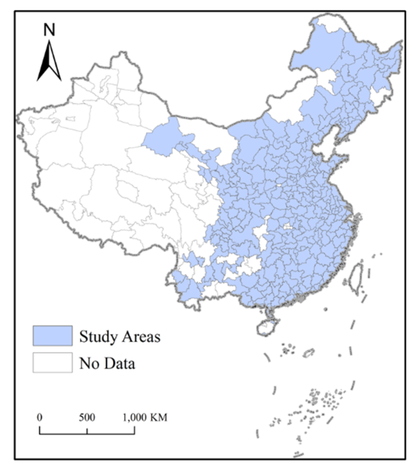
2.1. China’s City-Level PM2.5
2.2. Independent Variables
2.3. Global and Local Moran’s I
2.4. Rank von Neumann Ratio Test and Sample Autocorrelation Function
2.4.1. Rank von Neumann Ratio Test
2.4.2. Sample Autocorrelation Function
2.5. Multiscale Geographically Weighted Regression
2.6. Spatio-Temporal Lag
3. Results and Discussion
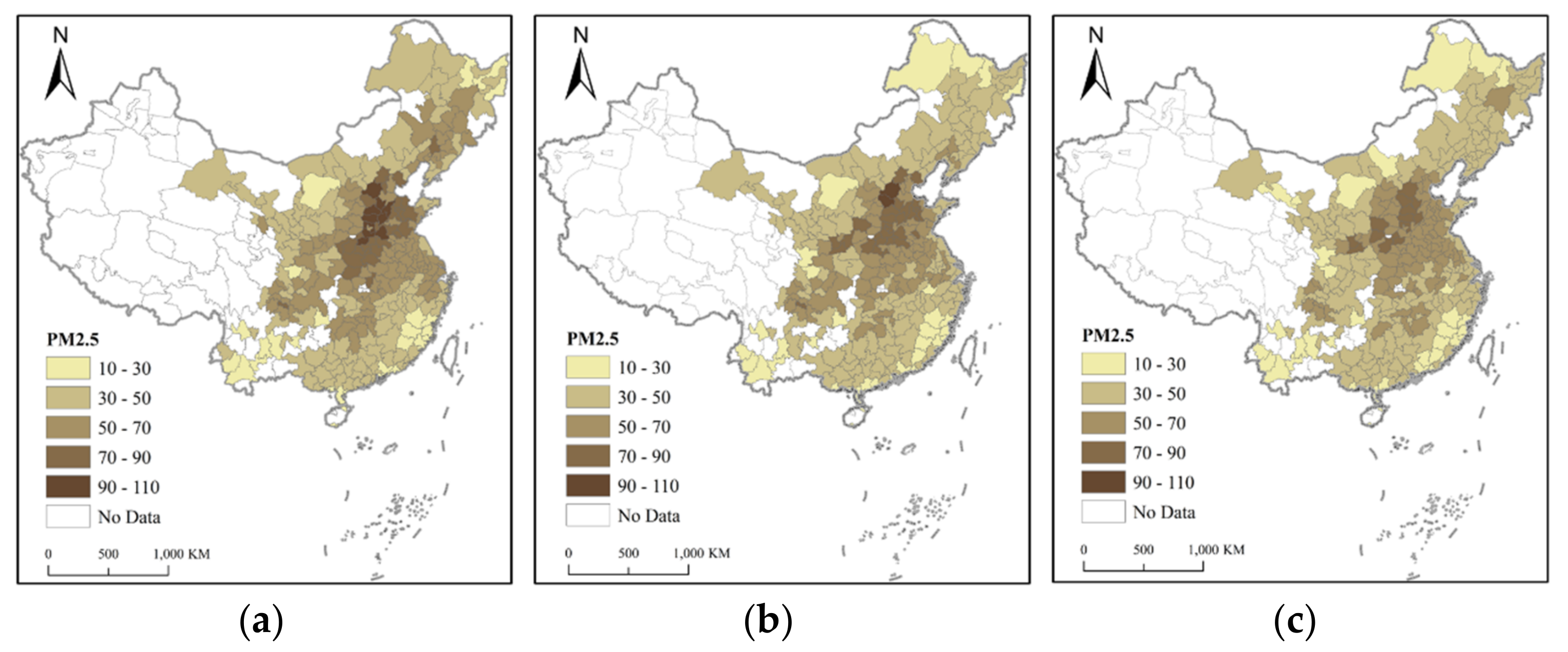
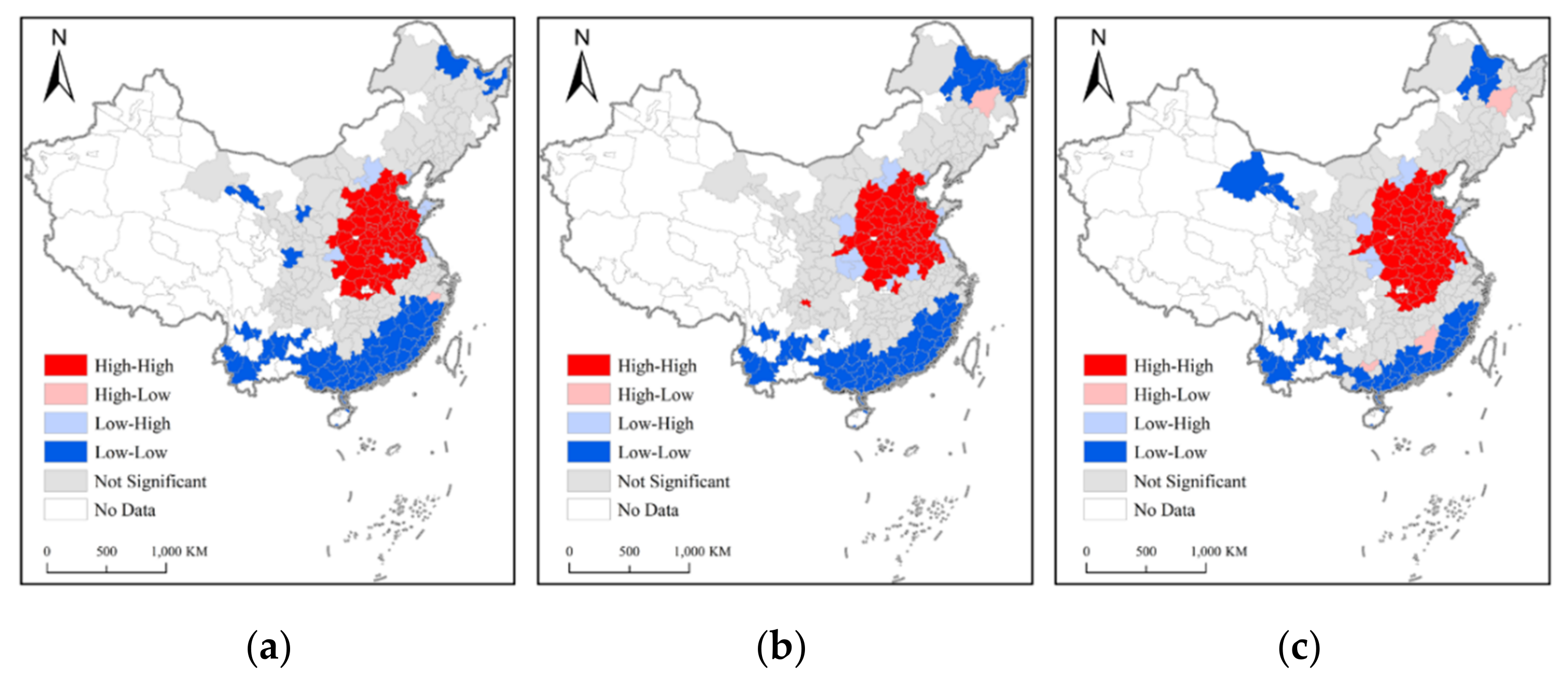
3.1. Spatial Patterns of PM2.5
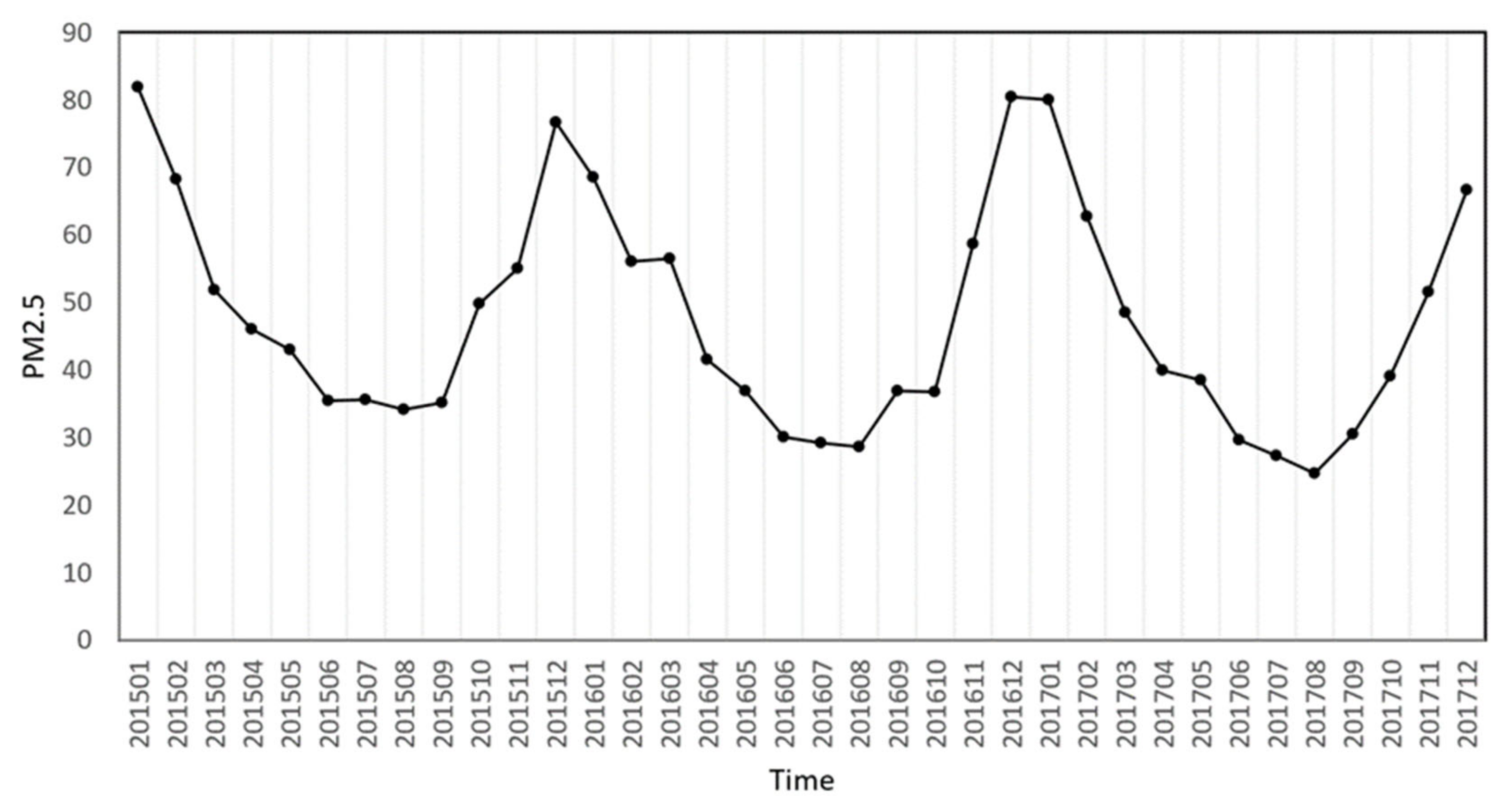
3.2. Temporal Patterns of PM2.5
3.3. Model Comparison
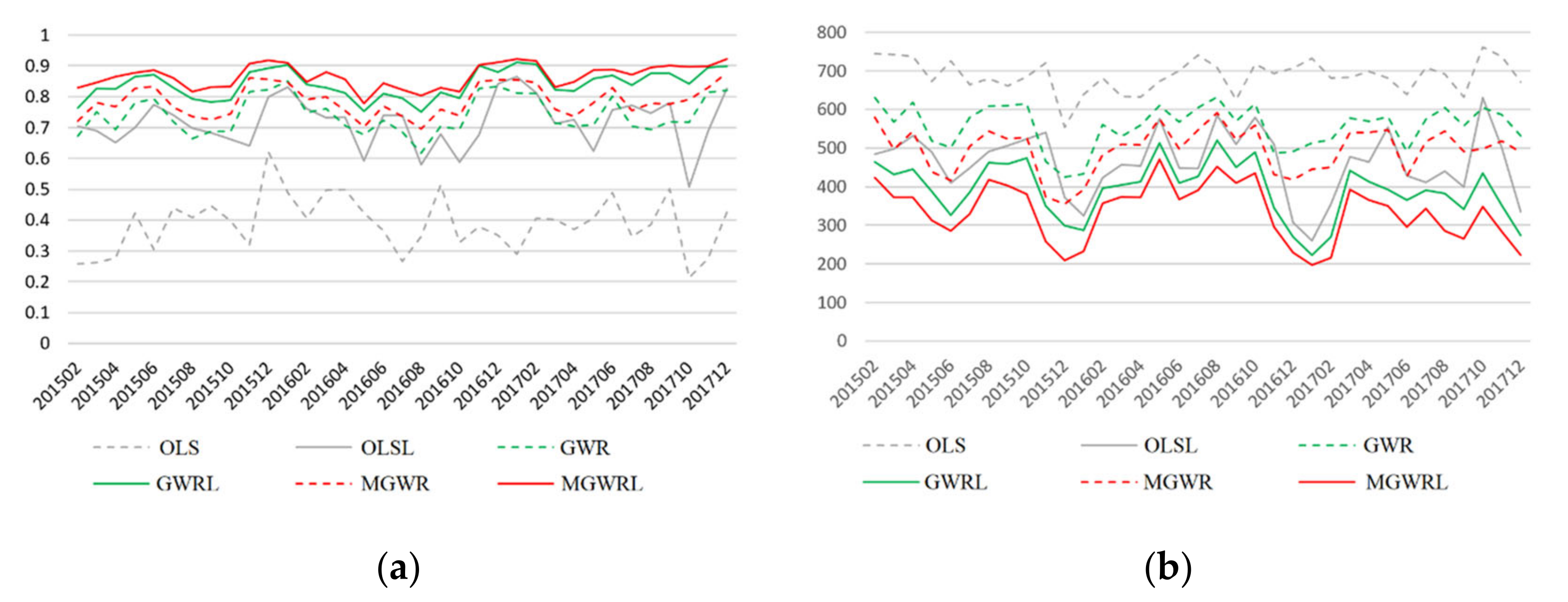
3.3.1. Goodness-of-Fit
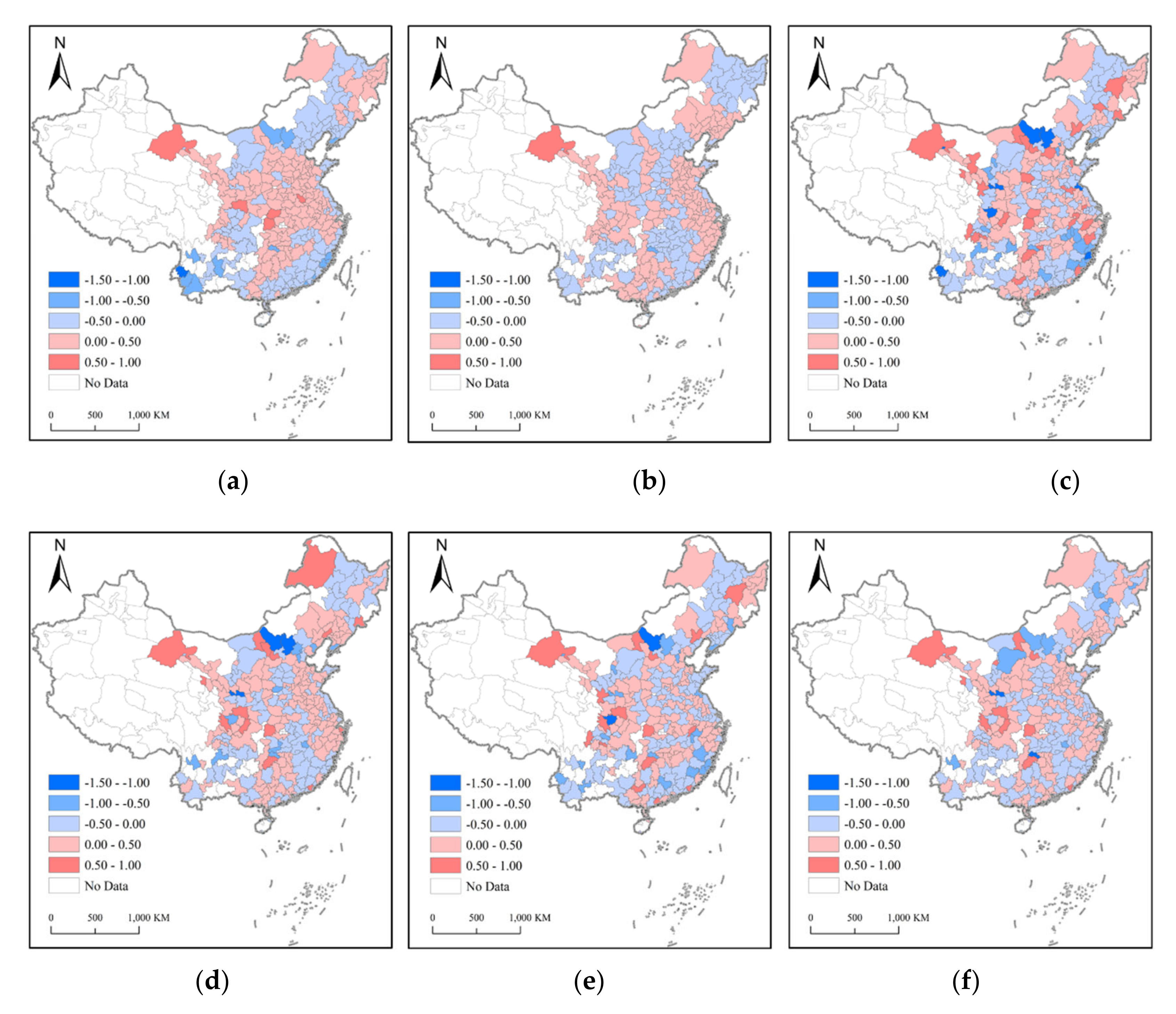
3.3.2. Residual Spatial Autocorrelation
3.4. Interpret Parameter Estimates
3.4.1. Results of OLSL
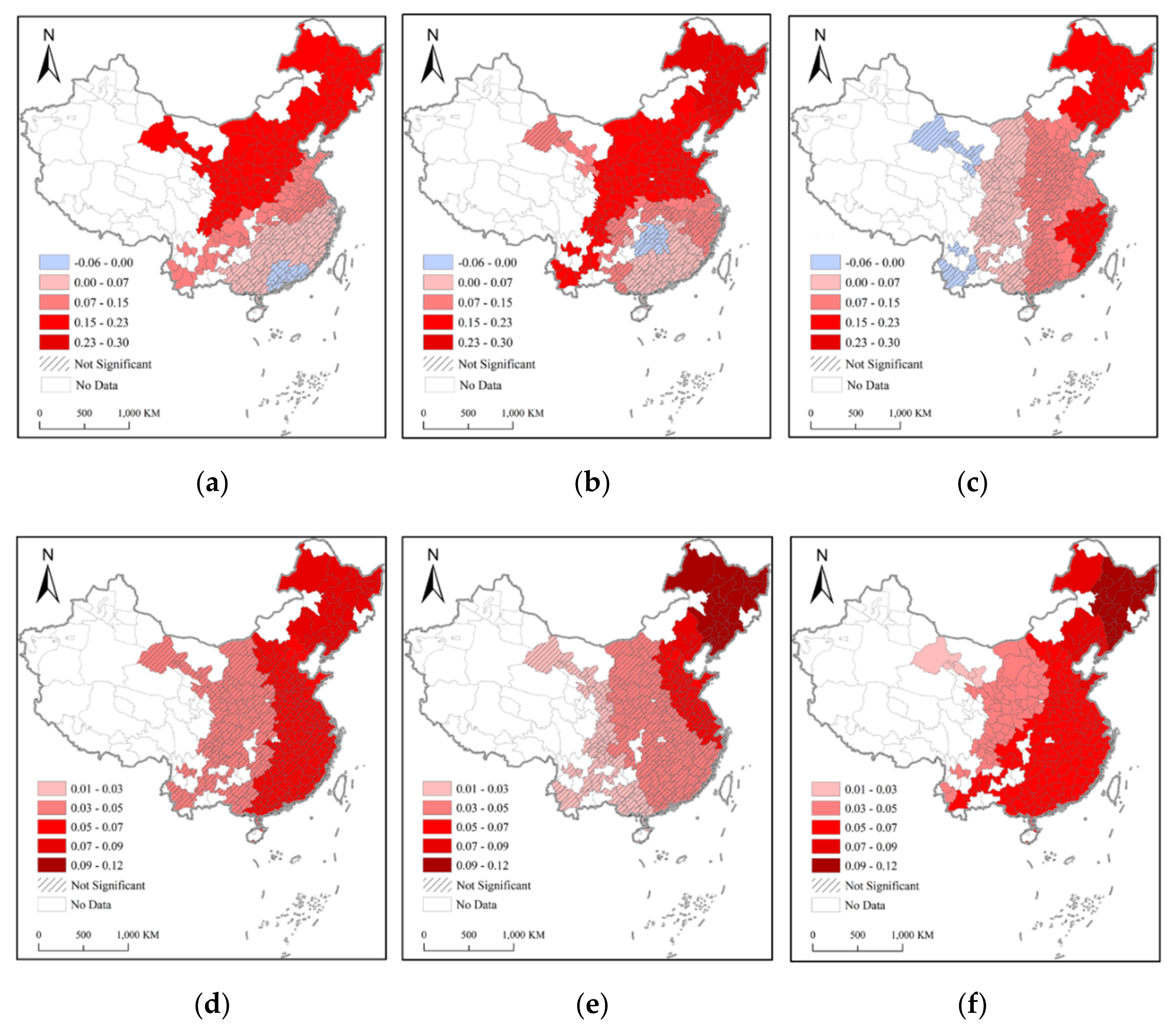
3.4.2. Results of MGWRL
4. Conclusions
Author Contributions
Funding
Conflicts of Interest
References
- Zhou, C.; Chen, J.; Wang, S. Examining the effects of socioeconomic development on fine particulate matter (PM2.5) in China’s cities using spatial regression and the geographical detector technique. Sci. Total Environ. 2018, 619–620, 436–445. [Google Scholar] [CrossRef] [PubMed]
- Yang, H.-H.; Lee, S.-A.; Hsieh, D.P.H.; Chao, M.-R.; Tung, C.-Y. PM2.5 and Associated Polycyclic Aromatic Hydrocarbon and Mutagenicity Emissions from Motorcycles. Bull. Environ. Contam. Toxicol. 2008, 81, 412–415. [Google Scholar] [CrossRef] [PubMed]
- Wang, S.; Zhou, C.; Wang, Z.; Feng, K.; Hubacek, K. The characteristics and drivers of fine particulate matter (PM2.5) distribution in China. J. Clean. Prod. 2017, 142, 1800–1809. [Google Scholar] [CrossRef]
- Adar, S.D.; Filigrana, P.A.; Clements, N.; Peel, J.L. Ambient Coarse Particulate Matter and Human Health: A Systematic Review and Meta-Analysis. Curr. Environ. Health Rep. 2014, 1, 258–274. [Google Scholar] [CrossRef] [Green Version]
- Thurston, G.D.; Ahn, J.; Cromar, K.R.; Shao, Y.; Reynolds, H.R.; Jerrett, M.; Lim, C.C.; Shanley, R.; Park, Y.; Hayes, R.B. Ambient Particulate Matter Air Pollution Exposure and Mortality in the NIH-AARP Diet and Health Cohort. Environ. Health Perspect. 2016, 124, 484–490. [Google Scholar] [CrossRef]
- Yeh, H.-L.; Hsu, S.-W.; Chang, Y.-C.; Chan, T.-C.; Tsou, H.-C.; Chang, Y.-C.; Chiang, P.-H. Spatial Analysis of Ambient PM2.5 Exposure and Bladder Cancer Mortality in Taiwan. Int. J. Environ. Res. Public Health 2017, 14, 508. [Google Scholar] [CrossRef]
- Feng, L.; Ye, B.; Feng, H.; Ren, F.; Huang, S.; Zhang, X.; Zhang, Y.; Du, Q.; Ma, L. Spatiotemporal Changes in Fine Particulate Matter Pollution and the Associated Mortality Burden in China between 2015 and 2016. Int. J. Environ. Res. Public Health 2017, 14, 1321. [Google Scholar] [CrossRef] [Green Version]
- Anselin, L. Spatial Econometrics: Methods and Models; Kluwer Academic: Dordrecht, The Netherlands, 1988. [Google Scholar]
- Fotheringham, A.S.; Brunsdon, C.; Charlton, M. Geographically Weighted Regression: The Analysis of Spatially Varying Relationships; John Wiley & Sons: Hoboken, NJ, USA, 2002. [Google Scholar]
- Jin, Q.; Fang, X.; Wen, B.; Shan, A. Spatio-temporal variations of PM2.5 emission in China from 2005 to 2014. Chemosphere 2017, 183, 429–436. [Google Scholar] [CrossRef]
- Lin, G.; Fu, J.; Jiang, D.; Hu, W.; Dong, D.; Huang, Y.; Zhao, M. Spatio-Temporal Variation of PM2.5 Concentrations and Their Relationship with Geographic and Socioeconomic Factors in China. Int. J. Environ. Res. Public Health 2014, 11, 173. [Google Scholar] [CrossRef] [Green Version]
- Wang, Z.-B.; Fang, C.-L. Spatial-temporal characteristics and determinants of PM2.5 in the Bohai Rim Urban Agglomeration. Chemosphere 2016, 148, 148–162. [Google Scholar] [CrossRef]
- Zhang, H.; Wang, Z.; Zhang, W. Exploring spatiotemporal patterns of PM2.5 in China based on ground-level observations for 190 cities. Environ. Pollut. 2016, 216, 559–567. [Google Scholar] [CrossRef]
- Cheng, Z.; Li, L.; Liu, J. Identifying the spatial effects and driving factors of urban PM2.5 pollution in China. Ecol. Indic. 2017, 82, 61–75. [Google Scholar] [CrossRef]
- Zhao, X.; Zhang, X.; Xu, X.; Xu, J.; Meng, W.; Pu, W. Seasonal and diurnal variations of ambient PM2.5 concentration in urban and rural environments in Beijing. Atmos. Environ. 2009, 43, 2893–2900. [Google Scholar] [CrossRef]
- Zheng, X.; Yu, Y.; Wang, J.; Deng, H. Identifying the determinants and spatial nexus of provincial carbon intensity in China: A dynamic spatial panel approach. Reg. Environ. Chang. 2014, 14, 1651–1661. [Google Scholar] [CrossRef] [Green Version]
- Pateraki, S.; Asimakopoulos, D.N.; Flocas, H.A.; Maggos, T.; Vasilakos, C. The role of meteorology on different sized aerosol fractions (PM10, PM2.5, PM2.5–10). Sci. Total Environ. 2012, 419, 124–135. [Google Scholar] [CrossRef]
- He, X.; Lin, Z.S. Interactive effects of the influencing factors on the changes of PM2.5 concentration based on gam model. Huanjing Kexue/Environ. Sci. 2017, 38, 22–32. [Google Scholar]
- Kadane, J.B.; Davidson, C.I. Using Statistical Regressions to Identify Factors Influencing PM2.5 Concentrations: The Pittsburgh Supersite as a Case Study AU-Chu, Nanjun. Aerosol Sci. Technol. 2010, 44, 766–774. [Google Scholar]
- Akbal, Y.; Unlu, K.D. A deep learning approach to model daily particular matter of Ankara: Key features and forecasting. Int. J. Environ. Sci. Technol. 2021. [Google Scholar] [CrossRef]
- Hao, Y.; Liu, Y.-M. The influential factors of urban PM2.5 concentrations in China: A spatial econometric analysis. J. Clean. Prod. 2016, 112, 1443–1453. [Google Scholar] [CrossRef]
- Elbayoumi, M.; Ramli, N.A.; Md Yusof, N.F.F.; Yahaya, A.S.B.; Al Madhoun, W.; Ul-Saufie, A.Z. Multivariate methods for indoor PM10 and PM2.5 modelling in naturally ventilated schools buildings. Atmos. Environ. 2014, 94, 11–21. [Google Scholar] [CrossRef]
- Yang, H.; Li, W.-W.; Kelly, K.E. Using a Continuous Time Lag to Determine the Associations between Ambient PM2.5 Hourly Levels and Daily Mortality AU-Staniswalis, Joan G. J. Air Waste Manag. Assoc. 2009, 59, 1173–1185. [Google Scholar]
- Liu, Y.; Paciorek, C.J.; Koutrakis, P. Estimating regional spatial and temporal variability of PM(2.5) concentrations using satellite data, meteorology, and land use information. Environ. Health Perspect. 2009, 117, 886–892. [Google Scholar] [CrossRef] [PubMed] [Green Version]
- Guan, D.; Su, X.; Zhang, Q.; Peters, G.P.; Liu, Z.; Lei, Y.; He, K. The socioeconomic drivers of China’s primary PM2.5 emissions. Environ. Res. Lett. 2014, 9, 024010. [Google Scholar] [CrossRef] [Green Version]
- Anselin, L.; Florax, R.J.; Rey, S.J. Advances in Spatial Econometrics: Methodology, Tools and Applications; Springer: Berlin, Germany, 2004. [Google Scholar]
- Hu, X.; Waller, L.A.; Al-Hamdan, M.Z.; Crosson, W.L.; Estes, M.G.; Estes, S.M.; Quattrochi, D.A.; Sarnat, J.A.; Liu, Y. Estimating ground-level PM2.5 concentrations in the southeastern U.S. using geographically weighted regression. Environ. Res. 2013, 121, 1–10. [Google Scholar] [CrossRef]
- Vardoulakis, S.; Kassomenos, P. Sources and factors affecting PM10 levels in two European cities: Implications for local air quality management. Atmos. Environ. 2008, 42, 3949–3963. [Google Scholar] [CrossRef]
- Anselin, L. Spatial econometrics. In A Companion to Theoretical Econometrics; Baltagi, B.H., Ed.; Blackwell: Oxford, UK, 1988; pp. 310–330. [Google Scholar]
- Fotheringham, A.S.; Yao, J. Local Spatiotemporal Modeling of House Prices: A Mixed Model Approach. Prof. Geogr. 2016, 68, 189–201. [Google Scholar]
- The Ministry of Ecology and Environment of PRC. Official Website of National Air Quality Daily. Available online: http://datacenter.mee.gov.cn (accessed on 3 February 2019).
- The National Meteorological Information Center. China Meteorological Data Service Centre. Available online: http://data.cma.cn (accessed on 3 February 2019).
- National Bureau of Statistics of China. China City Statistical Yearbook; China Statistics Press: Beijing, China, 2017. [Google Scholar]
- Moran, P.A. The interpretation of statistical maps. J. R. Stat. Society. Ser. B Methodol. 1948, 10, 243–251. [Google Scholar] [CrossRef]
- Cliff, A.D.; Ord, J.K. Spatial Processes: Models and Applications; Pion: London, UK, 1981. [Google Scholar]
- Anselin, L. Local Indicators of Spatial Association—LISA. Geogr. Anal. 1995, 27, 93–115. [Google Scholar] [CrossRef]
- Bartels, R. The Rank Version of von Neumann’s Ratio Test for Randomness. J. Am. Stat. Assoc. 1982, 77, 40–46. [Google Scholar] [CrossRef]
- Madansky, A. Prescriptions for Working Statisticians; Springer: New York, NY, USA, 1988. [Google Scholar]
- Chatfield, C. The Analysis of Time Series: An Introduction (6th Edition); Chapman and Hall: Boca Raton, FL, USA, 2004. [Google Scholar]
- Fotheringham, A.S.; Yang, W.; Kang, W. Multiscale Geographically Weighted Regression (MGWR). Ann. Am. Assoc. Geogr. 2017, 107, 1247–1265. [Google Scholar] [CrossRef]
- da Silva, A.R.; Fotheringham, A.S. The Multiple Testing Issue in Geographically Weighted Regression. Geogr. Anal. 2016, 48, 233–247. [Google Scholar] [CrossRef]
- Fotheringham, A.S.; Park, B. Localized Spatiotemporal Effects in the Determinants of Property Prices: A Case Study of Seoul. Appl. Spat. Anal. Policy 2018, 11, 581–598. [Google Scholar] [CrossRef]
- Lu, D.; Xu, J.; Yang, D.; Zhao, J. Spatio-temporal variation and influence factors of PM2.5 concentrations in China from 1998 to 2014. Atmos. Pollut. Res. 2017, 8, 1151–1159. [Google Scholar] [CrossRef]
- Okkaoğlu, Y.; Akdi, Y.; Ünlü, K.D. Daily PM10, periodicity and harmonic regression model: The case of London. Atmos. Environ. 2020, 238, 117755. [Google Scholar] [CrossRef]
- Zhang, Y.-L.; Cao, F. Is it time to tackle PM2.5 air pollutions in China from biomass-burning emissions? Environ. Pollut. 2015, 202, 217–219. [Google Scholar] [CrossRef]
- Remoundaki, E.; Papayannis, A.; Kassomenos, P.; Mantas, E.; Kokkalis, P.; Tsezos, M. Influence of Saharan Dust Transport Events on PM2.5 Concentrations and Composition over Athens. Water Air Soil Pollut. 2012, 224, 1373. [Google Scholar] [CrossRef]
- Li, L.; Qian, J.; Ou, C.-Q.; Zhou, Y.-X.; Guo, C.; Guo, Y. Spatial and temporal analysis of Air Pollution Index and its timescale-dependent relationship with meteorological factors in Guangzhou, China, 2001–2011. Environ. Pollut. 2014, 190, 75–81. [Google Scholar] [CrossRef]
- Stone, B. Urban sprawl and air quality in large US cities. J. Environ. Manag. 2008, 86, 688–698. [Google Scholar] [CrossRef]
- De Ridder, K.; Lefebre, F.; Adriaensen, S.; Arnold, U.; Beckroege, W.; Bronner, C.; Damsgaard, O.; Dostal, I.; Dufek, J.; Hirsch, J.; et al. Simulating the impact of urban sprawl on air quality and population exposure in the German Ruhr area. Part II: Development and evaluation of an urban growth scenario. Atmos. Environ. 2008, 42, 7070–7077. [Google Scholar] [CrossRef]
- Wang, S.; Fang, C.; Wang, Y. Spatiotemporal variations of energy-related CO2 emissions in China and its influencing factors: An empirical analysis based on provincial panel data. Renew. Sustain. Energy Rev. 2016, 55, 505–515. [Google Scholar] [CrossRef]
- Liang, X.; Zou, T.; Guo, B.; Li, S.; Zhang, H.; Zhang, S.; Huang, H.; Chen, S.X. Assessing Beijing’s PM2.5 pollution: Severity, weather impact, APEC and winter heating. Proc. R. Soc. A Math. Phys. Eng. Sci. 2015, 471, 20150257. [Google Scholar] [CrossRef] [Green Version]


| Variable | Definition | Mean | S.D. | Min | Max |
|---|---|---|---|---|---|
| pm25 | Monthly mean PM2.5 (μg/m3) | 46.62 | 25.32 | 5.06 | 254.1 |
| wind | Monthly mean wind velocity (m/s) | 2.17 | 0.72 | 0.50 | 7.64 |
| rain | Cumulative rainfall in a month (mm) | 93.95 | 101.82 | 0.00 | 855.05 |
| urban | Proportion of urban population (%) | 36.27 | 23.40 | 4.67 | 100 |
| popd | Population density (person/km2) | 438.14 | 339.72 | 5.73 | 2648.11 |
| pcgdp | Per capita GDP (104 yuan) | 5.11 | 2.96 | 1.01 | 21.54 |
| scgdp | Secondary industry as percentage to GDP (%) | 46.80 | 9.68 | 14.95 | 75.53 |
| dust | Volume of industrial dust emissions (104 ton) | 3.90 | 8.91 | 0.02 | 185.98 |
| psg | Highway passenger traffic in a year (108 person) | 0.66 | 1.20 | 0.01 | 15.69 |
| Stlag 1 | Spatiotemporal lag variable | 47.51 | 24.84 | 9.04 | 215.00 |
| 2015 | 2016 | 2017 | |
|---|---|---|---|
| Moran’s Index | 0.736 | 0.731 | 0.681 |
| Expected Index | −0.004 | −0.003 | −0.004 |
| z-score | 19.921 | 19.790 | 18.417 |
| p-value | <0.001 | <0.001 | <0.001 |
| Pattern | Clustered | Clustered | Clustered |
| OLS | OLSL | GWR | GWRL | MGWR | MGWRL | |||||||
|---|---|---|---|---|---|---|---|---|---|---|---|---|
| MI | z-Score | MI | z-Score | MI | z-Score | MI | z-Score | MI | z-Score | MI | z-Score | |
| 201701 | 0.248 *** | 30.682 | 0.066 *** | 8.582 | 0.034 *** | 4.679 | 0.004 | 0.964 | 0.011 | 1.794 | −0.011 | −0.859 |
| 201702 | 0.255 *** | 31.610 | 0.123 *** | 15.472 | 0.029 *** | 4.041 | 0.006 | 1.227 | −0.001 | 0.217 | −0.010 | −0.868 |
| 201703 | 0.156 *** | 19.512 | 0.071 *** | 9.202 | 0.021 ** | 3.088 | 0.005 | 1.128 | −0.005 | −0.249 | −0.009 | −0.790 |
| 201704 | 0.171 *** | 21.385 | 0.053 *** | 6.982 | 0.021 ** | 3.107 | 0.014 * | 2.228 | −0.002 | 0.108 | −0.010 | −0.845 |
| 201705 | 0.140 *** | 17.528 | 0.107 *** | 13.602 | 0.025 *** | 3.568 | 0.001 | 0.572 | 0.002 | 0.685 | −0.011 | −0.929 |
| 201706 | 0.230 *** | 28.585 | 0.114 *** | 14.422 | 0.032 *** | 4.395 | 0.024 *** | 3.443 | −0.001 | 0.215 | −0.003 | 0.035 |
| 201707 | 0.252 *** | 31.231 | 0.092 *** | 11.697 | 0.036 *** | 4.936 | 0.023 ** | 3.241 | −0.002 | 0.078 | −0.006 | −0.389 |
| 201708 | 0.199 *** | 24.692 | 0.111 *** | 14.052 | 0.029 *** | 4.004 | 0.007 | 1.363 | −0.007 | -0.458 | −0.012 | −1.079 |
| 201709 | 0.151 *** | 18.875 | 0.115 *** | 14.471 | 0.039 *** | 5.221 | 0.020 ** | 2.884 | 0.003 | 0.872 | −0.010 | −0.904 |
| 201710 | 0.198 *** | 24.601 | 0.112 *** | 14.186 | 0.022 ** | 3.222 | 0.012 * | 1.990 | 0.002 | 0.681 | −0.005 | −0.222 |
| 201711 | 0.167 *** | 20.867 | 0.184 *** | 22.877 | 0.010 | 1.665 | 0.014 * | 2.190 | 0.004 | 0.932 | −0.009 | −0.763 |
| 201712 | 0.200 *** | 19.865 | 0.199 *** | 9.844 | 0.075 ** | 2.858 | 0.011 | 1.784 | 0.001 | 0.186 | −0.005 | −0.248 |
| Variables | 201701 | 201702 | 201703 | 201704 | 201705 | 201706 | 201707 | 201708 | 201709 | 201710 | 201711 | 201712 |
|---|---|---|---|---|---|---|---|---|---|---|---|---|
| wind | −0.086 * | −0.051 | 0.022 | −0.040 | −0.151 ** | −0.073 | −0.078 | −0.085 | −0.072 | 0.095 | −0.270 *** | −0.124 *** |
| rain | 0.017 | −0.027 * | −0.036 *** | 0.011 | −0.125 *** | −0.135 *** | 0.001 | −0.091 *** | −0.048 *** | −0.108 *** | −0.012 | −0.010 * |
| urban | 0.046 * | −0.023 | −0.027 | −0.018 | 0.028 | −0.048 | −0.022 | 0.068 ** | 0.021 | 0.078 * | 0.018 | 0.025 |
| popd | 0.043 ** | 0.087 *** | 0.057 *** | 0.049 *** | 0.002 | 0.059 ** | 0.006 | 0.086 *** | 0.065 *** | 0.029 | 0.050 ** | 0.077 *** |
| pcgdp | −0.076 ** | −0.012 | 0.045 | 0.001 | −0.084 * | 0.017 | 0.017 | −0.008 | −0.041 | −0.121 ** | −0.111 *** | −0.085 *** |
| scgdp | 0.163 * | 0.191 ** | 0.047 * | 0.038 * | 0.034 ** | 0.039 * | 0.043 * | 0.082 * | 0.107 * | 0.181 * | 0.299 ** | 0.224 ** |
| dust | 0.010 | 0.025 * | 0.002 | 0.038 *** | 0.011 | 0.042 *** | 0.063 *** | 0.001 | 0.031 ** | 0.037 * | 0.001 | 0.021 * |
| psg | 0.027 * | 0.007 | 0.005 | 0.008 | 0.014 | 0.036 * | 0.034 * | 0.002 | 0.022 | 0.039 | 0.073 *** | 0.040 *** |
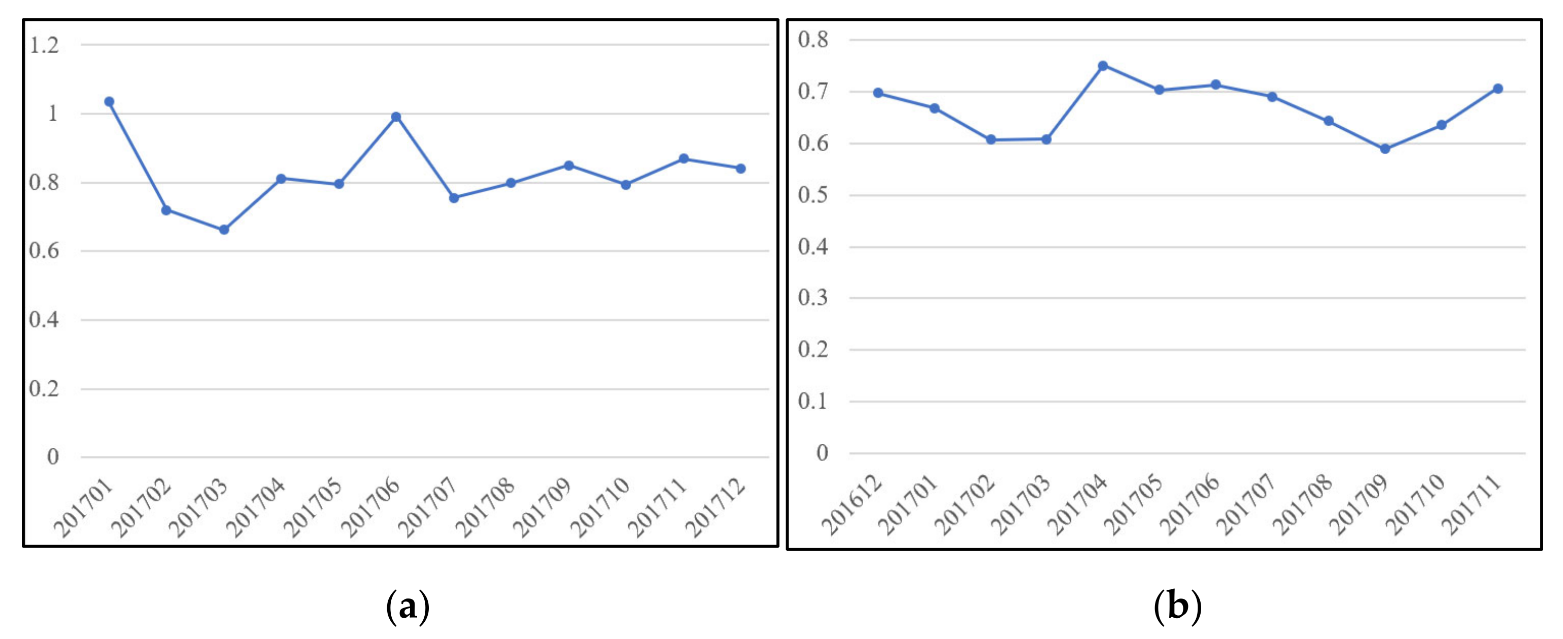
| stlag | 1.035 *** | 0.720 *** | 0.662 *** | 0.812 *** | 0.796 *** | 0.993 *** | 0.755 *** | 0.799 *** | 0.851 *** | 0.794 *** | 0.869 *** | 0.841 *** |
Publisher’s Note: MDPI stays neutral with regard to jurisdictional claims in published maps and institutional affiliations. |
© 2022 by the authors. Licensee MDPI, Basel, Switzerland. This article is an open access article distributed under the terms and conditions of the Creative Commons Attribution (CC BY) license (https://creativecommons.org/licenses/by/4.0/).
Share and Cite
Yue, H.; Duan, L.; Lu, M.; Huang, H.; Zhang, X.; Liu, H. Modeling the Determinants of PM2.5 in China Considering the Localized Spatiotemporal Effects: A Multiscale Geographically Weighted Regression Method. Atmosphere 2022, 13, 627. https://doi.org/10.3390/atmos13040627
Yue H, Duan L, Lu M, Huang H, Zhang X, Liu H. Modeling the Determinants of PM2.5 in China Considering the Localized Spatiotemporal Effects: A Multiscale Geographically Weighted Regression Method. Atmosphere. 2022; 13(4):627. https://doi.org/10.3390/atmos13040627
Chicago/Turabian StyleYue, Han, Lian Duan, Mingshen Lu, Hongsheng Huang, Xinyin Zhang, and Huilin Liu. 2022. "Modeling the Determinants of PM2.5 in China Considering the Localized Spatiotemporal Effects: A Multiscale Geographically Weighted Regression Method" Atmosphere 13, no. 4: 627. https://doi.org/10.3390/atmos13040627
APA StyleYue, H., Duan, L., Lu, M., Huang, H., Zhang, X., & Liu, H. (2022). Modeling the Determinants of PM2.5 in China Considering the Localized Spatiotemporal Effects: A Multiscale Geographically Weighted Regression Method. Atmosphere, 13(4), 627. https://doi.org/10.3390/atmos13040627