Article

Evaluation of WRF Cumulus Parameterization Schemes for the Hot Climate of Sudan Emphasizing Crop Growing Seasons

by
Abuelgasim I. I. Musa
1,2,*,
Mitsuru Tsubo
3,
Shaoxiu Ma
4,
Yasunori Kurosaki
3,
Yasuomi Ibaraki
5 and
Imad-Eldin A. Ali-Babiker
6,7
1
United Graduate School of Agricultural Science, Tottori University, Tottori 680-8550, Japan
2
Sudan Meteorological Authority, Khartoum 11115, Sudan
3
Arid Land Research Center, Tottori University, Tottori 680-8550, Japan
4
International Platform for Dryland Research and Education, Tottori University, Tottori 680-8550, Japan
5
Faculty of Agriculture, Yamaguchi University, Yamaguchi 753-8511, Japan
6
Agricultural Research Corporation, Khartoum 11115, Sudan
7
Higher Council for Environment and Natural Resources, Khartoum 11115, Sudan
*
Author to whom correspondence should be addressed.
Atmosphere 2022, 13(4), 572; https://doi.org/10.3390/atmos13040572
Submission received: 10 February 2022 / Revised: 25 March 2022 / Accepted: 31 March 2022 / Published: 2 April 2022
(This article belongs to the Section Climatology)

Abstract

:
High spatiotemporal resolution climate data are essential for climate-related impact studies. The Weather Research and Forecasting (WRF) model is widely used to downscale climate data for different regions with regional-specific physics configurations. This study aimed to identify robust configurations of the WRF model, especially cumulus parameterization schemes, for different climatic zones of Sudan. We focused on wet season (June–September) rainfall and dry season (November–February) temperature, which are determinants of summer crop and irrigated wheat yields, respectively. Downscaling experiments were carried out to compare the following schemes: Betts–Miller–Janjic (BMJ), improved Kain–Fritch (KFT), modified Tiedtke (TDK), and Grell–Freitas (GF). Results revealed that the BMJ performed better for wet season rainfall in the hyper-arid and arid zones; KFT performed better for rainfall in July and August in the semi-arid zone where most summer crops are cultivated. For dry season temperature, the BMJ and TDK outperformed the other schemes in all three zones, except that the GF performed best for the minimum temperature in December and January in the arid zone, where irrigated wheat is produced, and in the semi-arid zone. Specific parameterization schemes therefore need to be selected for specific seasons and climatic zones of Sudan.

1. Introduction

High spatial resolution climate data are required for local-scale impact assessments of climate variability and changes of ecosystem services. The outputs of general circulation models (GCMs) are not sufficient for such local-scale studies, and therefore regional climate models (RCMs), which incorporate detailed specifications of the earth’s surface such as land use and water bodies, have been broadly applied to satisfy this requirement. RCMs outperform GCMs in detailed simulation of mesoscale processes, e.g., convective rainfall processes [1,2,3]. Weather Research and Forecasting (WRF) is a well-known RCM used for many purposes such as operational forecasting and dynamical downscaling. As local climates are regulated by global circulations and further constrained by land surface conditions, the WRF model provides multiple physics options to satisfy region-dependent climate conditions. Numerous studies have been conducted with the aim of identifying robust configurations of physical processes for specific scales and geographical locations and their applications [4,5,6,7,8,9].
Previous studies have tested various physical options of the WRF model to identify the most suitable configurations for specific regions. For example, over the Middle East and North Africa (MENA), the climates of which are hot and dry, rainfall is sensitive mainly to cumulus parameterization physics such as the Kain–Fritsch scheme (KF) [10], the Grell–Devenyi ensemble scheme (GD) [11] and the Betts–Miller–Janjic scheme (BMJ) [12], whereas microphysics such as the Goddard scheme (GODDARD) [13] and the WRF Single-moment 6-class scheme (WSM6) [14] significantly affect temperature deviations [15]. However, the model outputs are less sensitive to planetary boundary layer physics, such as the Mellor–Yamada–Janjic scheme (MYJ) [12] and the Yonsei University scheme (YSU) [16], than to cumulus parameterization physics and microphysics [15]. In the case of shortwave and longwave radiation physics, the Community Atmosphere Model (CAM) [17] and Rapid Radiative Transfer Model for GCMs (RRTMG) [18] capture well the inter-annual variability and warming trends of temperature, but they are season- and location-dependent over MENA [19]. A previous study [20] has further indicated that temperature is sensitive to land surface physics such as the Noah land surface model (NOAH) [21], NOAH with multi-parameterization (NOAHMP) [22], Community Land Model (CLM) [23], and the Rapid Update Cycle (RUC) [24]. The following configuration of the WRF model has been recommended for MENA: CAM or RRTMG, NOAH, YSU, the WRF Single-moment 5-class scheme for microphysics (WSM5) or WSM6, and KF [15,19,20].
The sensitivity of the WRF model outputs to the physics options has been reported for the neighboring regions of MENA, i.e., the Nile River basin and the Eastern Nile basin. The configuration recommended for the Nile River basin is a combination of the Dudhia scheme for shortwave radiation (DUDHIA) [25] and the Rapid Radiative Transfer Model for longwave radiation (RRTM) [26], NOAH, MYJ, the WRF Single-moment 3-class scheme for microphysics (WSM3) [27], and KF [28]. For the Eastern Nile basin, the climates of which are wetter than those of MENA, a set of CAM, NOAH, MYJ, WSM6, and BMJ is recommended [29]. In the case of rainfall, the WRF model outputs are very sensitive to the cumulus parameterization option [15,28,29,30,31,32]. There are two types of cumulus parameterization options: adjustment and mass-flux. The BMJ is a typical adjustment type, whereas the GD and KF are examples of the widely used mass-flux type. The WRF model with the adjustment type does not simulate detailed processes of cumulus convection. Instead, it uses a simplified process that involves adjusting lapse rates of temperature and humidity. Compared with the adjustment type, the mass-flux type is complex because it involves cloud modelling for cumulus convective processes. The model performance with this type depends mainly on the reproduction of entrainment/detrainment and/or updrafts/downdrafts. The performance of WRF downscaling experiments has been reported from different regions of Africa. For example, the BMJ outperforms the GD in South Africa [30], where it reproduces the intensity of summer rainfall anomalies, and the KF and GD over Central and Western Africa [31]. Over East Africa, model simulation with the KT incorporating a moisture-advection-based trigger function (KFT) as well as the KT and GD [33] outperforms model simulation with the BMJ [32].
In Northeast Africa, drought and extremely high temperature events often occur and negatively affect crop production. Sudan is one of the countries vulnerable to such climate risks: droughts impact summer crops such as sorghum and pearl millet during the wet season from June to September in the relatively wet climate of the southern part [34], and high temperatures affect irrigated wheat during the dry season from November to February in the dry climate of the central and northern parts [35]. Rainfall is a critical climate element in the wet season because summer crops are cultivated under rainfed conditions. Lack of rain results in crop failure, hence the economic loss. In the dry season, wheat is produced under irrigated conditions due to no rain falling in the cultivated areas, but the crop is often exposed to heat stress. Previous studies have shown that yields of the summer crops are positively associated with rainfall in the wet season [34], and irrigated wheat yield is negatively associated with temperature in the dry season [35]. The main objective of this study was therefore to identify a robust configuration of the WRF model for generating high-spatial-resolution climate data for crop growing seasons in Sudan. The focus was on wet season rainfall and dry season temperature. The specific objectives were (1) to compare downscaled rainfall and temperature data between cumulus parameterization schemes and (2) to determine cumulus parameterization schemes for specific growing seasons and climatic zones.

2. Materials and Methods
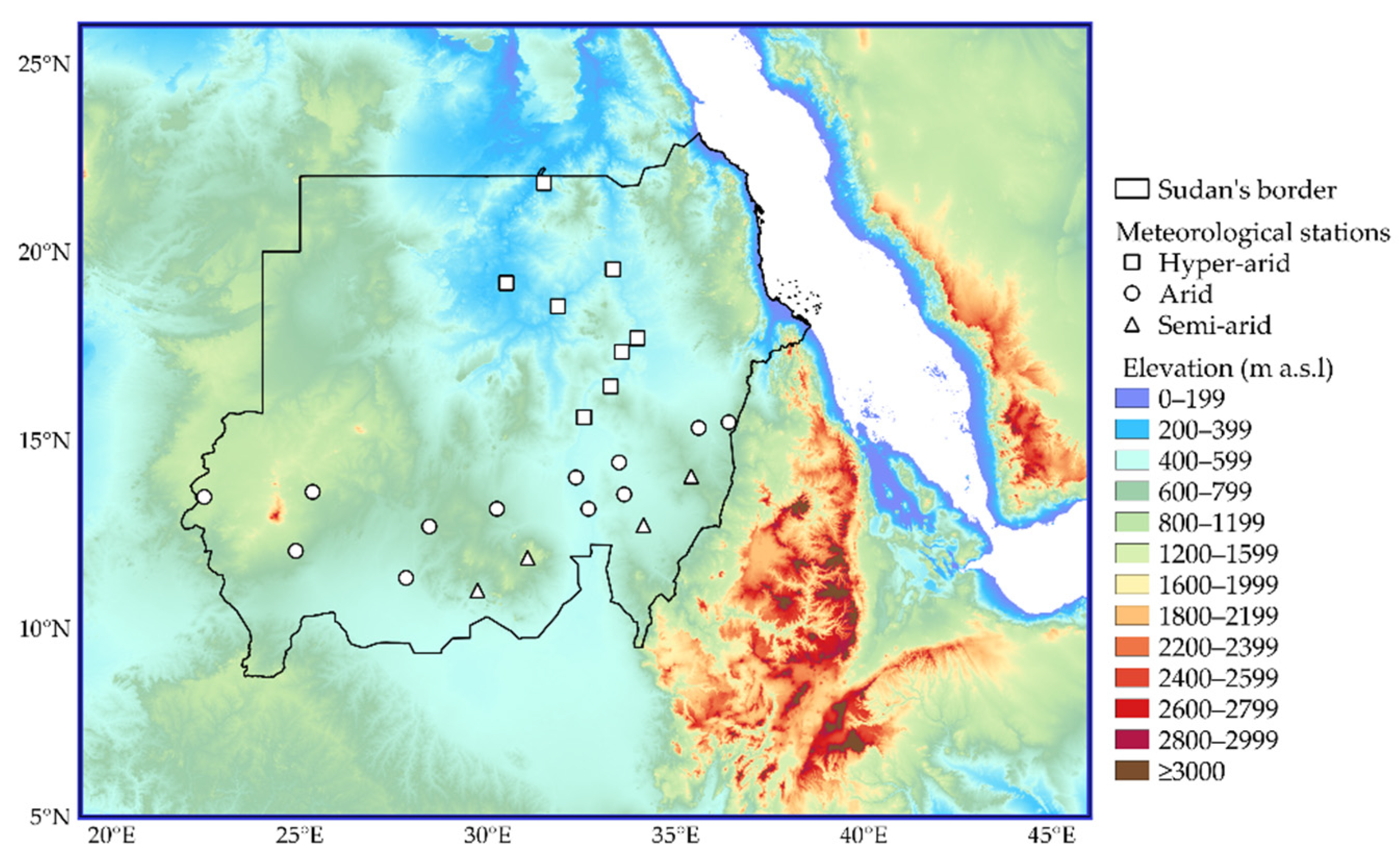
2.1. Study Area

Sudan is one of the most water-scarce countries in the world. Based on the aridity index [36], the Sudan can be divided into three aridity zones, hyper-arid, arid, and semi-arid. These zones are all characterized by hot, wet summers and relatively cold, dry winters. In general, northern Sudan receives less rainfall and experiences larger temperature changes between seasons than southern Sudan. For example, Dongola (19.17° N, 30.48° E) receives less than 15 mm of annual rainfall, and the range of monthly mean temperatures is 17.6–34.5 °C; the annual rainfall at Wad Medani (14.40° N, 33.48° E) is about 300 mm, and the range of monthly mean temperatures is 23.6–33.1 °C; at Gedaref (14.03° N, 35.40° E), the annual rainfall is about 600 mm, and the range of monthly mean temperatures is 25.9–32.7 °C. These sites are in the hyper-arid, arid, and semi-arid zones, respectively [37]. The topography of Sudan is relatively flat, except in the southwestern part (Figure 1).

2.2. Model Configuration

We used the WRF model version 4.2 (Advanced Research WRF). The BMJ scheme has been commonly selected in WRF downscaling experiments in the Nile River basin and the Eastern Nile basin [28,29]. The KFT scheme, the Tiedtke scheme [38], and the Grell–Freitas scheme (GF) [39] perform well to some extent in the neighboring regions of Sudan, i.e., East Africa [32,40] and West Africa [41]. However, to the best of our knowledge, the KFT, Tiedtke, and GF are never tested in the study area. Therefore, the following schemes were selected to evaluate the sensitivity of model outputs to cumulus parameterization: (a) BMJ [12], an adjustment type of the convection scheme introduced by Betts and Miller [42]; (b) KFT [33], an improved mass-flux scheme of Kain and Fritsch [43] based on Fritsch and Chappell [44] for a convective system of detrainment from clouds; (c) a modified Tiedtke (TDK) scheme [45], a modification of the mass-flux scheme of Tiedtke [38] with respect to entrainment and detrainment in cumulus convection; and (d) GF [39], a mass-flux scheme with the stochastic approach of Grell and Dévényi [11] based on Grell’s [46] original scheme. The other four physics schemes selected for this study were the RRTMG, unified NOAH [47], YSU, and WSM6 for shortwave and longwave radiation physics, land surface physics, planetary boundary layer physics, and microphysics, respectively. These were chosen based on recommendations found in previous studies of Northeast Africa [15,19,20,28,29,32].

2.3. Model Simulation

A set of experiments was run to test these cumulus parameterization schemes using 6-hourly data from the National Centers for Environmental Prediction (NCEP)-Climate Forecast System Reanalysis (CFSR) at a horizontal resolution of 0.5° × 0.5° [48]. The NCEP-CFSR dataset is available for the period 1979–2010 from the Research Data Archive of Computational and Information Systems Laboratory of the National Center for Atmospheric Research (ds093.0) (https://rda.ucar.edu) (accessed on 19 March 2021). In this study, the downscaling experiments were carried out for 10 years from 2000 to 2010 by running the model from May of each year to May of the following year. The NCEP-CFSR data were downscaled to 10 km horizontal resolution for a single domain centered over Sudan (Figure 1) using the WRF Preprocessing System version 4 consisting of the 10 min surface topography data (slope category, terrain height, soil type, soil temperature) of the United States Geological Survey and the land use data (albedo, vegetation fraction, land use classification,) of the Moderate Resolution Imaging Spectroradiometer (MODIS) (https://www2.mmm.ucar.edu/wrf/users/download/get_sources_wps_geog.html) (accessed on 20 November 2020).

2.4. Model Validation

Daily rainfall data and maximum and minimum temperatures (TMAX and TMIN, respectively) at 24 meteorological stations (Figure 1) were obtained from the Sudan Meteorological Authority. Annual, seasonal, and monthly averages of daily rainfall, TMAX, and TMIN were used to evaluate model performance. For seasonal and monthly comparisons, wet season (June–September) and dry season (November–February) data were used for rainfall and temperature, respectively. TMAX was also used for the comparisons for the wet season in relation to heat stress to crops. Moreover, the number of rainy days (NRD) (daily rainfall ≥ 1 mm) in the wet season and the frequency of hot days (FHD) (daily TMAX > 35 °C) in the dry season was used as drought and extreme temperature indices, respectively.
Model validation was performed using the data averaged over the meteorological stations located in each climatic zone. For statistical analysis of the downscaling experiments, a Taylor Diagram was used to depict the similarity between the experimental outputs and the corresponding observed data (10 years). The diagram showed the Pearson correlation coefficient (R), standard deviation (SD), and root-mean-square error (RMSE) [49]. The significance of the correlation coefficient was tested at p ≤ 0.05 (2-tailed). We normalized both the SD of the simulated data and the RMSE to the SD of the observed data. The spatial distributions of the simulated rainfall and temperature data were also compared with the 10-year average satellite-based reanalysis data, i.e., the Integrated Multi-Satellite Retrievals for GPM (IMERG) [50] (https://gpm.nasa.gov) (accessed on 17 May 2021) for rainfall at a horizontal resolution of 0.1° × 0.1° and the Modern-Era Retrospective analysis for Research and Applications, Version 2 (MERRA2) [51] (https://gmao.gsfc.nasa.gov) (accessed on 26 April 2021) for temperature at a horizontal resolution of 0.5° × 0.625°. The IMERG database has been developed since 2000, using the data collected with the TRMM/GPM onboard Dual-frequency Precipitation Radar and Microwave Imager together with other passive microwave radiometers such as GCOM-W1 AMSR2 and NOAA-20 ATMS. The MERRA2 dataset (1980 to present) has been generated on a cubed-sphere grid with the GEOS General Circulation Model.

3. Results

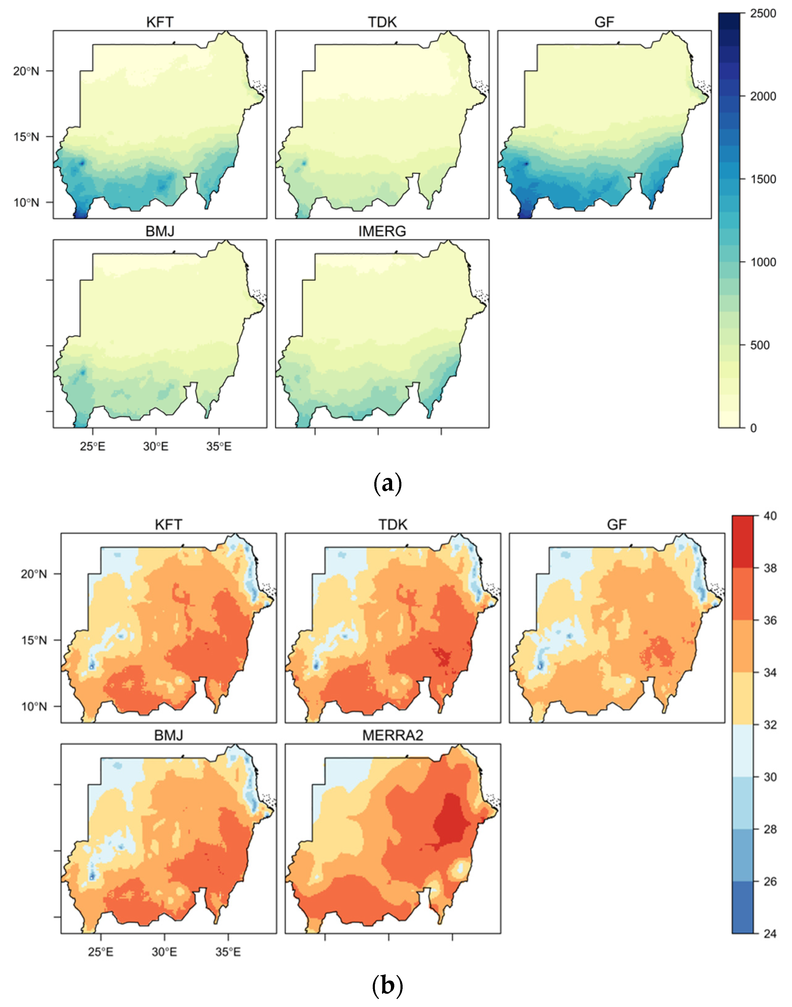
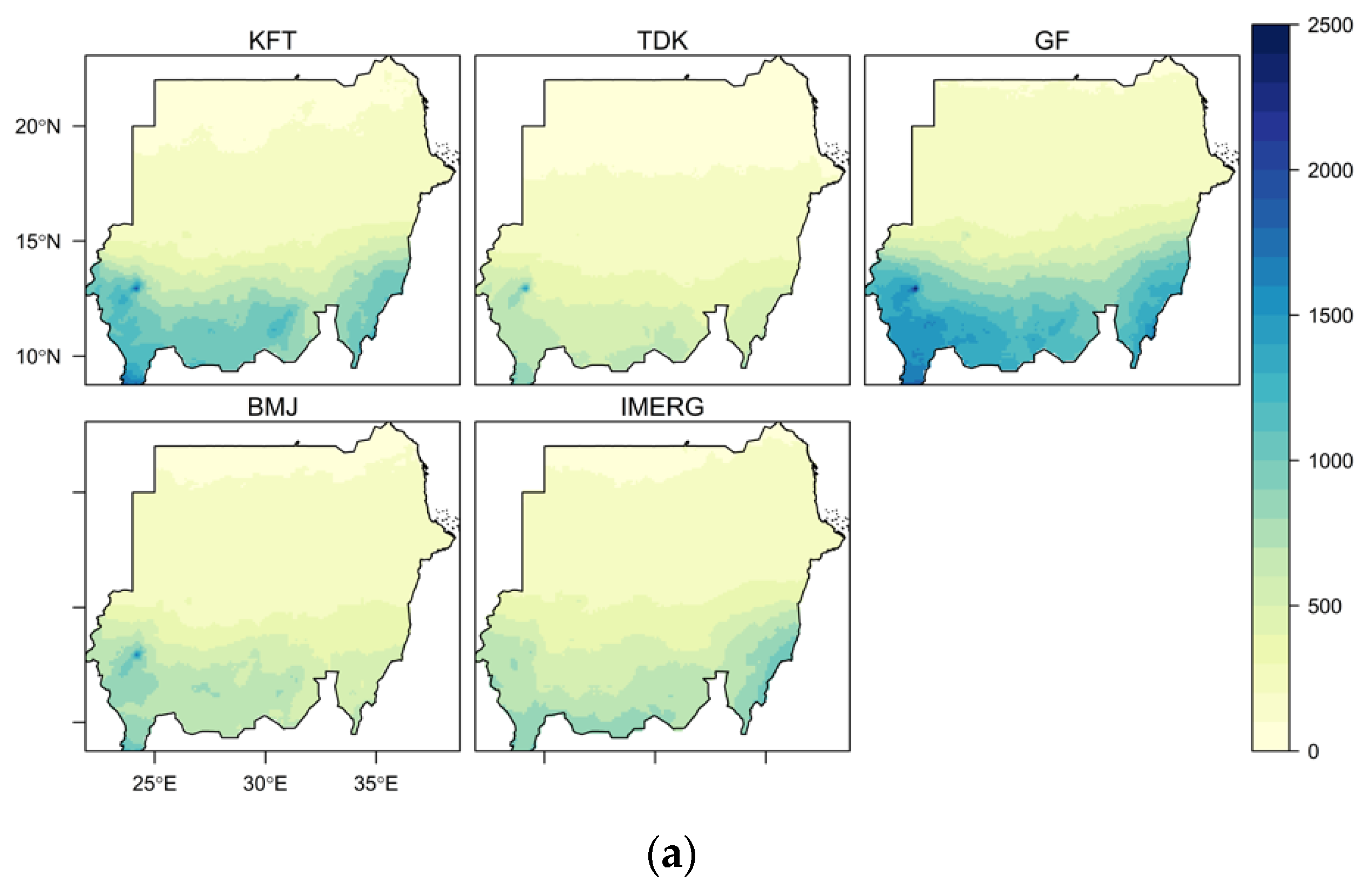
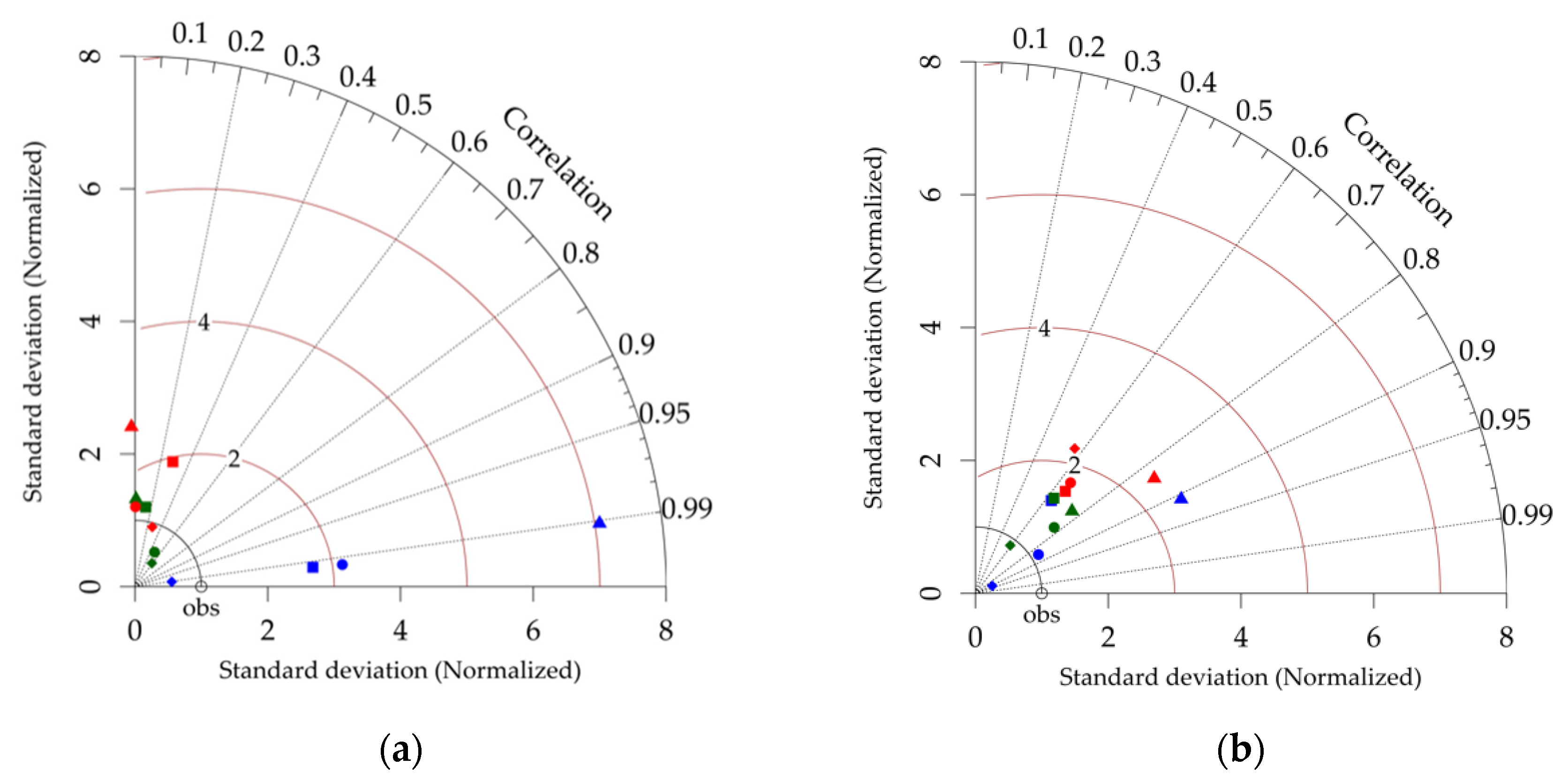
3.1. Annual Rainfall and Temperature

Figure 2a shows the spatial distribution of annual rainfall. The simulated data and the satellite-based data were comparable in the central to northern part of the study area. The rainfall simulated with the BMJ scheme most closely agreed with the satellite-based data (IMERG) (Figure 2a, Figures S1a and S2a, Table 1). Use of the KFT and GF schemes resulted in slight overestimates of rainfall in southern Sudan, and the rainfall simulated by the TDK was low in northern Sudan. In southeastern Sudan, the KFT-simulated rainfall was more-or-less in agreement with the satellite-based data. All four schemes produced results that were very strongly correlated with the satellite-based data (R = 0.92 for BMJ, 0.96 for KFT, 0.93 for TDK, 0.97 for GF). The normalized SD for the BMJ scheme was close to unity. The BMJ scheme had the lowest RMSE, followed by the TDK and then the KFT scheme (Table 1).
Figure 2b shows the spatial distribution of the annual TMAX (Figures S1b and S2b). The distributions simulated with the BMJ, KFT, and TDK schemes were comparable with the MERRA2 data, except in the northeastern corner of Sudan, whereas the GF reproduced the low TMAX in the central to southern and central to eastern parts of the Sudan. All four schemes simulated temperatures that were strongly correlated with the satellite-based data, and the normalized SD was close to unity (Table 1). The RMSEs of the temperatures simulated by the KFT and TDK were lower than the corresponding RMSEs of the BMJ and GF. Like TMAX, the simulated TMIN was strongly correlated with the satellite-based data, and the normalized SD was close to unity (Table 1). However, the RMSE was higher for TMIN than for TMAX in all four schemes. The simulated TMIN was higher than the satellite-based TMIN over the study area (Figure 2c, Figures S1c and S2c).

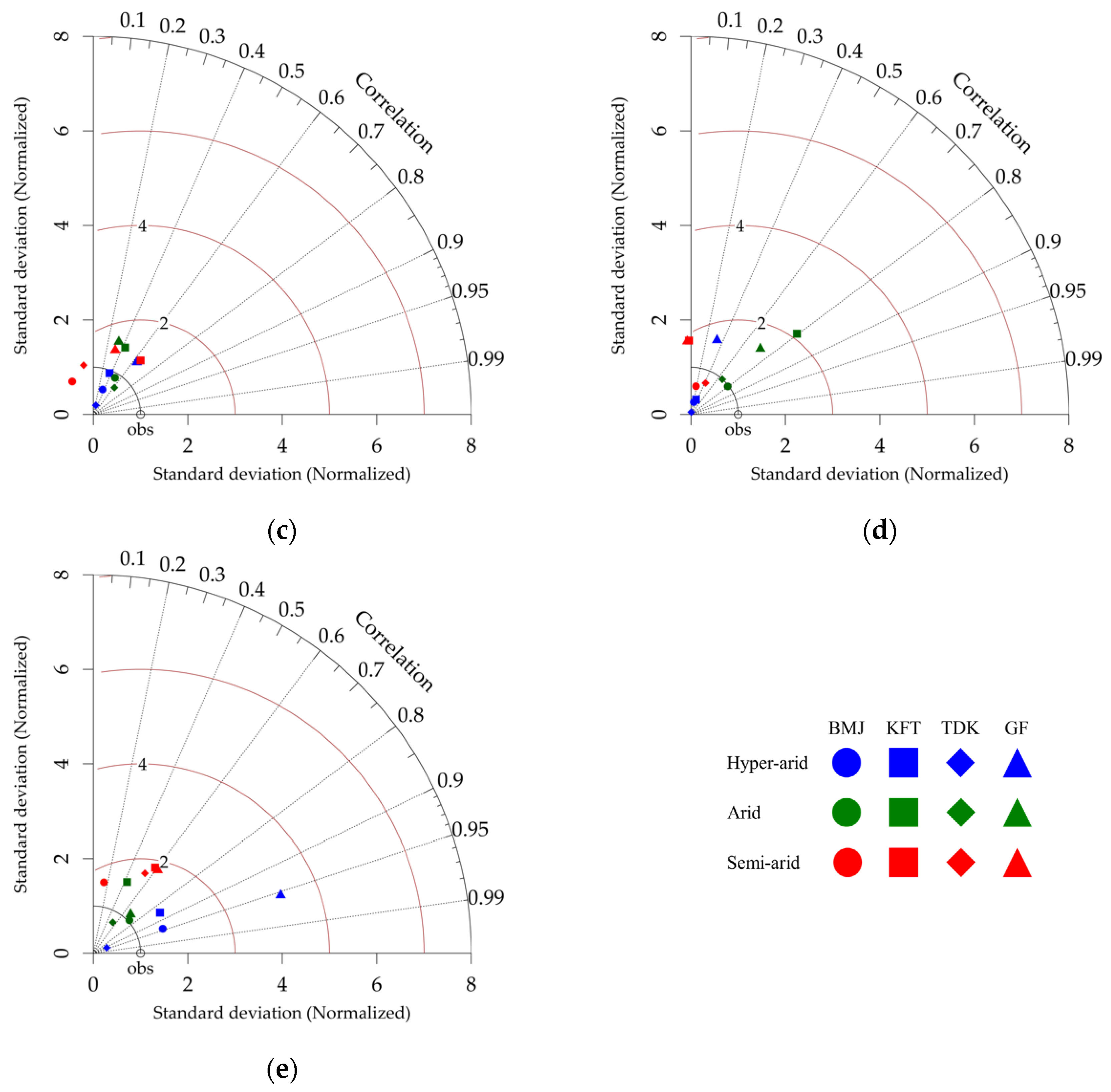
3.2. Wet Season Rainfall and Temperature

Figure 3a shows the spatial distribution of the wet season (June–September) rainfall (Figure S3a). Like annual rainfall, the wet season rainfall simulated with the BMJ scheme was highly consistent with the IMERG data. The wet season rainfall simulated by all four schemes was very strongly correlated with the satellite-based rainfall (R = 0.91 for BMJ, 0.96 for KFT, 0.92 for TDK, 0.97 for GF). The RMSE of the wet season rainfall simulated by the BMJ was the lowest among the schemes. The variance of the BMJ rainfall was low, and its normalized SD was close to unity (Table 1). Figure 4 shows Taylor diagrams of monthly and seasonal rainfall to allow comparisons between climatic zones. The seasonal rainfall simulated by all the schemes was significantly correlated with observed seasonal rainfall in the hyper-arid zone (R = 0.94 for BMJ, 0.85 for KFT, 0.93 for TDK, 0.96 for GF). The simulated NRD also agreed with the observed data for TDK (R = 0.81) and GF (R = 0.68) (Table 2). The simulated monthly rainfall was also in agreement with the observed rainfall in June and July, and the GF-simulated rainfall was significantly correlated with the observed rainfall in August (Figure 4). In all months, both the SD and RMSE were higher for the GF-simulated rainfall than for the other schemes. In the arid zone, correlations were high between the seasonal rainfall simulated with the BMJ and GF schemes and the observed rainfall. The BMJ-simulated NRD was also consistent with the observed data (R = 0.64), but no correlation was found between GF-simulated and observed NRDs (Table 2). There were significant correlations between observed and simulated monthly rainfall for all four schemes in July and September, except for the TDK in July, but there were no analogous correlations in June and August (Figure 4). In general, the SD and RMSE were lower for the BMJ- and TDK-simulated rainfall than for the KFT- and GF-simulated rainfall. In the semi-arid zone, no correlations were found between simulated and observed seasonal rainfall, but KFT-simulated monthly rainfall was significantly correlated with observed rainfall in July and August. The BMJ- and GF-simulated rainfalls were consistent with the observed rainfall in July. In addition, the TDK-simulated NRD was significantly correlated with the observed data (R = 0.71) (Table 2). The SD and RMSE of the simulated rainfall were relatively high in the semi-arid zone compared with the hyper-arid and arid zones (Figure 4).
The seasonal TMAX simulated by all four schemes was very strongly correlated with the observed data in the hyper-arid zone (R > 0.8) (Table 2). In the arid and semi-arid zones, the simulated TMAX was also significantly correlated with the observed data.

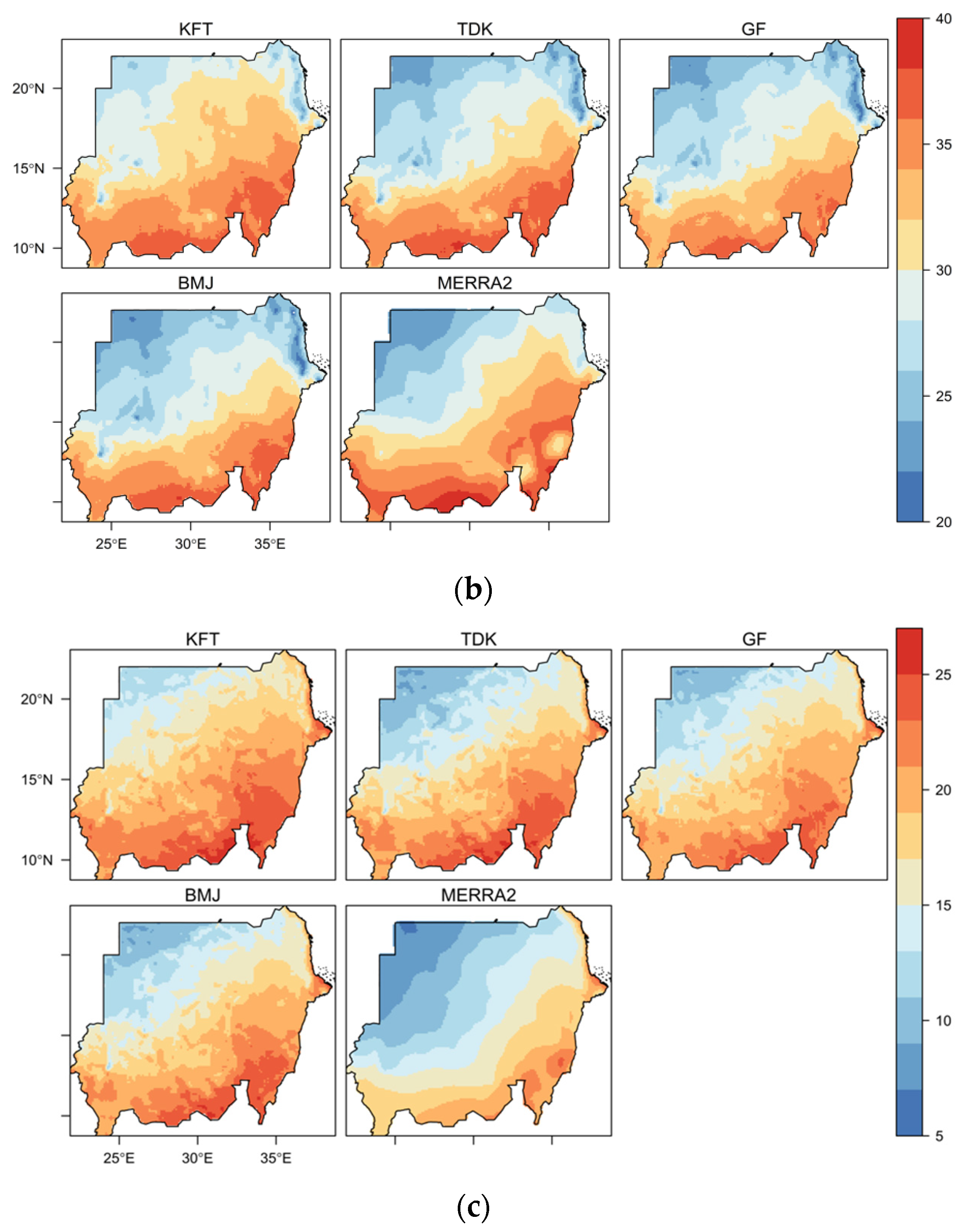
3.3. Dry Season Maximum Temperature

Figure 3b shows the spatial distribution of the dry season (November–February) TMAX (Figure S3b). The distributions simulated with the BMJ, TDK, and GF schemes were comparable to that of the MERRA2 data. The KFT-simulated TMAX values were relatively high, particularly in northwestern Sudan, and its RMSEs were higher than those of the other schemes (Table 1). The seasonal TMAX values were more highly correlated than the annual TMAX values with the MERRA2 data (R = 0.93 for BMJ, 0.91 for KFT, 0.94 for TDK, 0.93 for GF). The Taylor diagrams further showed that the simulated TMAX agreed with the observed data, except for KFT, in all three zones (Figure 5). Similarly, the FHDs simulated by all four schemes were strongly correlated with the observed data in all three zones (Table 2). The normalized SDs for BMJ and TDK were close to unity. The RMSEs were higher for the KFT and GF than for the BMJ and TDK schemes. The simulated monthly TMAX was significantly correlated with the observed data, except for the following schemes and months: KFT for December and January, TDK for November, and GF for November and January in the hyper-arid zone; KFT for January and GF for November and January in the arid zone; and BJM and TDK for November and KFT and GF for January in the semi-arid zone.

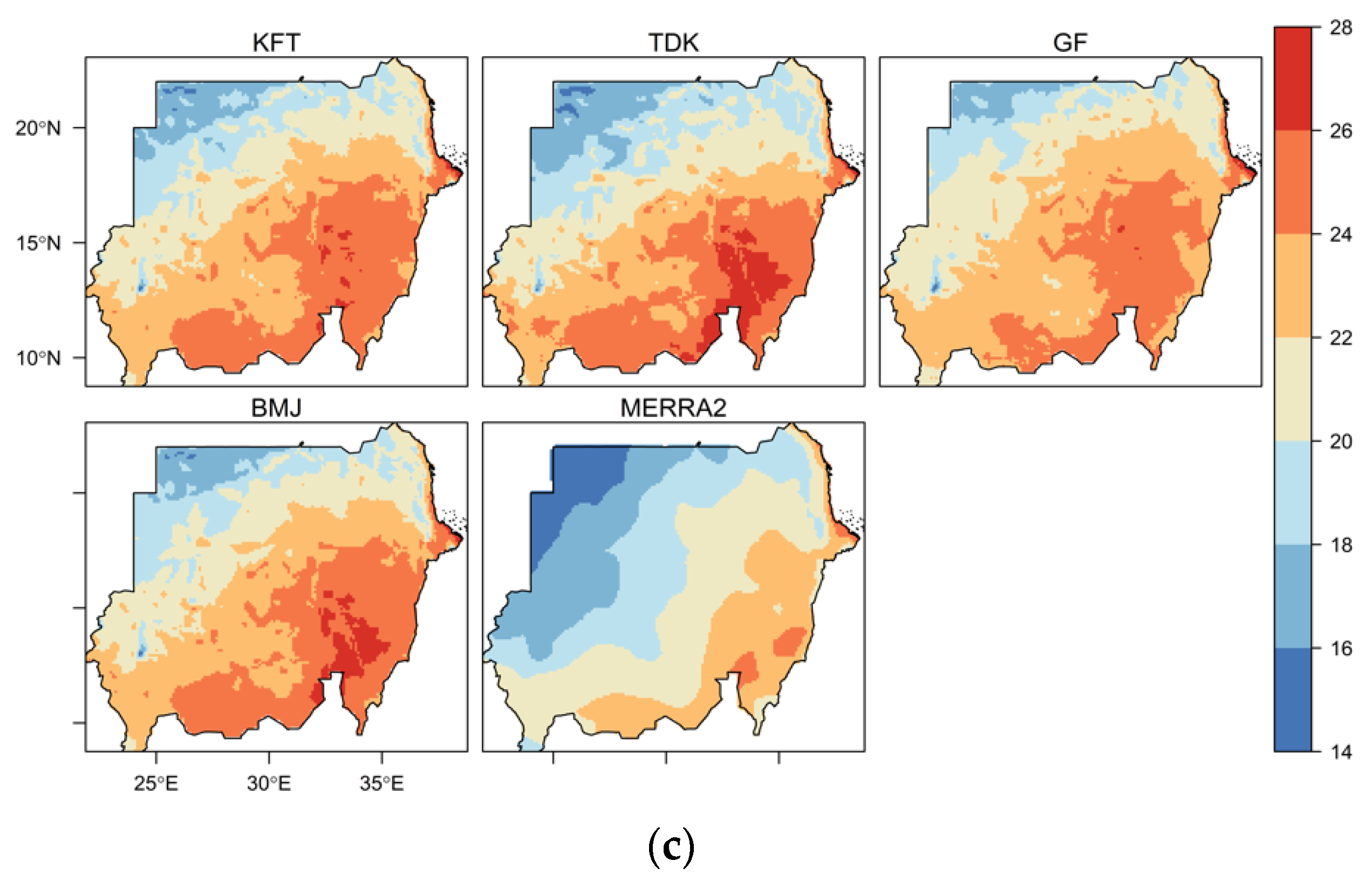
3.4. Dry Season Minimum Temperature

Figure 3c shows the spatial distribution of the dry season TMIN (Figure S3c). Like TMAX, the spatial distributions of the TMINs simulated with the BMJ, TDK, and GF schemes were comparable to those of the MERRA2 data, but the TMINs simulated by the KFT scheme were relatively high. The TMINs simulated by all four schemes were strongly correlated with the reanalysis data (MERRA2) (R = 0.94 for BMJ, 0.93 for KFT, 0.94 for TDK, 0.94 for GF), and the normalized SDs were near unity (Table 1). In contrast to the TMAX values, the RMSEs were relatively high, except for KFT. The Taylor diagrams also showed that the BMJ- and TDK-simulated seasonal TMINs were in agreement with the observed data in all three zones (Figure 6). However, the GF-simulated TMINs were not correlated with the observed data in the hyper-arid zone, and the KFT-simulated TMINs were correlated with the observed data only in the arid zone. The RMSEs associated with the seasonal TMIN data were relatively high compared to the RMSEs of the TMAX data. The normalized SDs were close to unity in the arid zone but lower than unity in the hyper-arid and semi-arid zones. The monthly TMINs simulated by all four schemes were in agreement with the observed TMIN in February in all three zones, December in the hyper-arid zone, and November in the arid zone. In addition, the TMINs simulated with the following schemes and months were significantly correlated with the observed TMINs in the arid and semi-arid zones: BMJ in December, TDK in November and December, and GF in December and January.

4. Discussion

Our modeling experiments revealed that different cumulus parameterization schemes of the WRF model led to different model performance for Sudan. The adjustment type scheme (BMJ) performed better than the mass-flow type schemes (KFT, TDK, and GF) (Figure 2a and Figure 3a). This result was not consistent with the results of previous studies in the Nile River basin [28] and the MENA [15], where the KF outperformed the BMJ. This difference could be attributed to differences in landscapes as well as land cover between these regions. In addition, the fact that the KFT outperformed the BMJ scheme in southeastern Sudan indicates that mass-flux schemes could be used for downscaling over regions of relatively high rainfall in the study area. In the case of the spatial distribution of temperature, the model outputs of both annual and seasonal temperatures were less sensitive to the cumulus parameterization option in the study area (Figure 2b,c and Figure 3b,c). This conclusion agrees with the results of previous studies of the Nile River basin [28] and MENA [15].
Comparisons between climatic zones revealed that the model performance differed between the cumulus parameterization schemes for wet season rainfall (Figure 4). The BMJ outperformed the other schemes for wet season rainfall in the hyper-arid and arid zones. In the semi-arid zone, all four schemes performed relatively poorly for seasonal rainfall, but the mass-flow (KFT) scheme performed better for the main months of the growing season (July and August). This result is consistent with the results of a previous study of cumulus parameterization options for seasonal rainfall in East Africa [32]. That study considered the same physics options as this study, and the results showed that mass-flow schemes (KF, KFT, and GD) performed better than the adjustment-type scheme (BMJ). In the case of dry season temperature, the BMJ and TDK schemes outperformed the KFT and GF schemes for TMAX in all three zones (Figure 5). In the arid and semi-arid zones, the GF performed better for TMIN during the growing season and its main months (December and January), but the BMJ and TDK outperformed the GF for the seasonal TMIN in the hyper-arid zone (Figure 6). This result is partly consistent with the results of a previous study in the Eastern Nile basin, which considered different schemes of the two other physics options (CAM for radiation and MYJ for planetary boundary layer). In that study, the BMJ outperformed the KF and GD schemes [29]. These results indicate that the model outputs are sensitive to the types of cumulus parameterization options, and the best option depends on the other physics options considered. Previous studies of WRF downscaling for Northeast Africa [28,29,32] have indicated that the best WRF configuration depends on the type of climate and confirms that the best cumulus parameterization scheme is region-dependent for both rainfall and temperature in the study area. The schemes that performed best for downscaling rainfall during the wet season were the BJM for the hyper-arid and arid zones and the KFT for the semi-arid zone. In the case of dry season temperature, the BMJ and TDK should be used in all climatic zones, but the GF can be selected for TMIN in the arid and semi-arid zones.
The sensitivity of the WRF model outputs to the choice of physics options has been reported from Northeast Africa. For example, the WSM6 performs better than other microphysics schemes such as GODDARD, WSM3, and WSM5 [15,29], and NOAH performs better than other land surface schemes such as NOAHMP, CLM, and RUC [20,28]. In the case of the planetary boundary layer option, MYJ performs better than YSU over the Nile River basin [28] and the Eastern Nile basin [29], whereas the latter performs better than the former over MENA [15]. In the case of the radiation physics option, a set of DUDHIA and RRTM performs better than CAM over the Nile River basin [28], whereas the latter performs better than the former over the Eastern Nile basin [29]. The performance of the radiation physics schemes (CAM and RRTMG) for temperature varies from location to location and from season to season over MENA [19]. In this study, the other physics options were fixed to test the cumulus parameterization options. Accordingly, further downscaling experiments for the study area (Sudan) are recommended to evaluate the radiation physics and planetary boundary layer options in particular; for example, RRTMG and YSU can be compared with CAM and MYJ, respectively.

5. Conclusions

This study evaluated cumulus parameterization options of the WRF model to determine the most robust configuration for a relatively small domain centered over Sudan. The downscaling of the NCEP-CFSR data was sensitive to four schemes, i.e., BMJ, KFT, TDK, and GF. This physics option should be carefully selected for generating high-spatial-resolution climate data in the study area. The major production areas of summer crops lie in the semi-arid zone, whereas irrigated wheat is cultivated mostly in the arid and hyper-arid zones. As rainfall and temperature are determinants of the climatic conditions for summer crops and irrigated wheat, respectively, the recommended schemes for cumulus parameterization are therefore the KFT for wet season rainfall in the semi-arid zone, and either the BMJ or TDK for the dry season temperature in the hyper-arid and arid zones, except for the dry season TMIN in the arid zone, for which the GF is recommended. The cumulus parameterization scheme thus needs to be selected separately for each climatic zone in Sudan.

Supplementary Materials

The following supporting information can be downloaded at: https://www.mdpi.com/article/10.3390/atmos13040572/s1, Figure S1. Spatial distributions of the differences between the 10-year average annual rainfall (mm) and maximum and minimum temperatures (°C) simulated with the Betts–Miller–Janjic (BMJ), improved Kain–Fritch (KFT), modified Tiedtke (TDK), and Grell–Freitas (GF) schemes, and IMERG [50] observed rainfall data and MERRA2 [51] observed temperature data in Sudan. The differences were calculated by subtracting the observed data from the simulated data; Figure S2. Histograms of the 10-year average annual rainfall (mm) and maximum and minimum temperatures (°C) simulated with the Betts–Miller–Janjic (BMJ), improved Kain–Fritch (KFT), modified Tiedtke (TDK), and Grell–Freitas (GF) schemes, and IMERG [50] observed rainfall data and MERRA2 [51] observed temperature data in Sudan; Figure S3. Histograms of the 10-year seasonal (June–September) rainfall (mm) and seasonal (November–February) maximum and minimum temperatures (°C) simulated with the Betts–Miller–Janjic (BMJ), improved Kain–Fritch (KFT), modified Tiedtke (TDK), and Grell–Freitas (GF) schemes, and IMERG [50] observed rainfall data and MERRA2 [51] observed temperature data in Sudan.

Author Contributions

Conceptualization, A.I.I.M., M.T. and S.M.; methodology, A.I.I.M., M.T. and S.M.; data analysis, A.I.I.M.; writing—original draft preparation, A.I.I.M.; writing—review and editing, M.T., S.M., Y.K., Y.I. and I.-E.A.A.-B. All authors have read and agreed to the published version of the manuscript.

Funding

This study was funded by the Science and Technology Research Partnership for Sustainable Development, Japan Science and Technology Agency/Japan International Cooperation Agency (JPMJSA1805).

Institutional Review Board Statement

Not applicable.

Informed Consent Statement

Not applicable.

Data Availability Statement

Not applicable. All data are available from the sources.

Acknowledgments

We are grateful to the Sudan Meteorological Authority for providing the data.

Conflicts of Interest

The authors declare no conflict of interest.

References

  1. Wilby, R.L.; Wigley, T.M.L. Downscaling general circulation model output: A review of methods and limitations. Prog. Phys. Geogr. 1997, 21, 530–548. [Google Scholar] [CrossRef]
  2. Soares, P.M.M.; Cardoso, R.M.; Miranda, P.M.A.; de Medeiros, J.; Belo-Pereira, M.; Espirito-Santo, F. WRF high resolution dynamical downscaling of ERA-Interim for Portugal. Clim. Dyn. 2012, 39, 2497–2522. [Google Scholar] [CrossRef]
  3. Garcia-Carreras, L.; Challinor, A.J.; Parkes, B.J.; Birch, C.E.; Nicklin, K.J.; Parker, D.J. The impact of parameterized convection on the simulation of crop processes. J. Appl. Meteorol. Climatol. 2015, 54, 1283–1296. [Google Scholar] [CrossRef]
  4. Fu, C.; Wang, S.; Xiong, Z.; Gutowski, W.J.; Lee, D.K.; McGregor, J.L.; Sato, Y.; Kato, H.; Kim, J.W.; Suh, M.S. Regional Climate Model Intercomparison Project for Asia. Bull. Am. Meteorol. Soc. 2005, 86, 257–266. [Google Scholar] [CrossRef] [Green Version]
  5. Christensen, J.H.; Carter, T.R.; Rummukainen, M. Evaluating the performance and utility of regional climate models: The PRUDENCE project. Clim. Chang. 2007, 81, 1–6. [Google Scholar] [CrossRef]
  6. Giorgi, F.; Jones, C.; Asrar, G.R. Addressing climate information needs at the regional level: The CORDEX framework. WMO Bull. 2009, 58, 175–183. [Google Scholar]
  7. Van der Linden, P.; Mitchell, J.F.B. ENSEMBLES, Climate Change and Its Impacts: Summary of Research and Results from the ENSEMBLES Project; Met Office Hadley Centre: Exeter, UK, 2009; 160p.
  8. Mearns, L.O.; Sain, S.; Leung, L.R.; Bukovsky, M.S.; McGinnis, S.; Biner, S.; Caya, D.; Arritt, R.W.; Gutowski, W.; Takle, E.; et al. Climate Change Projections of the North American Regional Climate Change Assessment Program (NARCCAP). Clim. Chang. 2013, 120, 965–975. [Google Scholar] [CrossRef] [Green Version]
  9. Solman, S.A.; Sanchez, E.; Samuelsson, P.; da Rocha, R.P.; Li, L.; Marengo, J.; Pessacg, N.L.; Remedio, A.R.C.; Chou, S.C.; Berbery, H.; et al. Evaluation of an ensemble of regional climate model simulations over South America driven by the ERA-Interim reanalysis: Model performance and uncertainties. Clim. Dyn. 2013, 41, 1139–1157. [Google Scholar] [CrossRef]
  10. Kain, J.S. The Kain-Fritsch convective parameterization: An update. J. Appl. Meteorol. 2004, 43, 170–181. [Google Scholar] [CrossRef] [Green Version]
  11. Grell, G.A.; Dévényi, D. A generalized approach to parameterizing convection combining ensemble and data assimilation techniques. Geophys. Res. Lett. 2002, 29, 31–38. [Google Scholar] [CrossRef] [Green Version]
  12. Janjić, Z.I. The step-mountain eta coordinate model: Further developments of the convection, viscous sublayer, and turbulence closure schemes. Mon. Weather Rev. 1994, 122, 927–945. [Google Scholar] [CrossRef] [Green Version]
  13. Tao, W.K.; Simpson, J.; McCumber, M. An ice–water saturation adjustment. Mon. Weather Rev. 1989, 117, 231–235. [Google Scholar] [CrossRef] [Green Version]
  14. Hong, S.Y.; Lim, J.O.J. The WRF single-moment 6-class microphysics scheme (WSM6). Asia-Pac. J. Atmos. Sci. 2006, 42, 129–151. [Google Scholar]
  15. Zittis, G.; Hadjinicolaou, P.; Lelieveld, J. Comparison of WRF model physics parameterizations over the MENA-CORDEX domain. Am. J. Clim. Chang. 2014, 3, 490–511. [Google Scholar] [CrossRef] [Green Version]
  16. Hong, S.Y.; Noh, Y.; Dudhia, J. A new vertical diffusion package with an explicit treatment of entrainment processes. Mon. Weather Rev. 2006, 134, 2318–2341. [Google Scholar] [CrossRef] [Green Version]
  17. Collins, W.D.; Rasch, P.J.; Boville, B.A.; Hack, J.J.; McCaa, J.R.; Williamson, D.L.; Briegleb, B.P.; Bitz, C.M.; Lin, S.J.; Zhang, M. The formulation and atmospheric simulation of the Community Atmosphere Model Version 3 (CAM3). J. Clim. 2006, 19, 2144–2161. [Google Scholar] [CrossRef] [Green Version]
  18. Iacono, M.J.; Delamere, J.S.; Mlawer, E.J.; Shephard, M.W.; Clough, S.A.; Collins, W.D. Radiative forcing by long-lived greenhouse gases: Calculations with the AER radiative transfer models. J. Geophys. Res. 2008, 113, D13103. [Google Scholar] [CrossRef]
  19. Zittis, G.; Hadjinicolaou, P. The effect of radiation parameterization schemes on surface temperature in regional climate simulations over the MENA-CORDEX domain. Int. J. Climatol. 2017, 37, 3847–3862. [Google Scholar] [CrossRef]
  20. Constantinidou, K.; Hadjinicolaou, P.; Zittis, G.; Lelieveld, J. Performance of land surface schemes in the WRF model for climate simulations over the MENA-CORDEX domain. Earth Syst. Environ. 2020, 4, 647–665. [Google Scholar] [CrossRef]
  21. Mitchell, K.; Ek, M.; Wong, V.; Lohmann, D.; Koren, V.; Schaake, J.; Duan, Q.; Gayno, G.; Moore, B.; Grunmann, P.; et al. Noah land Surface Model (LSM) User’s Guide; NCAR Research Application Laboratory: Boulder, CO, USA, 2005; 26p. [Google Scholar]
  22. Niu, G.Y.; Yang, Z.L.; Mitchell, K.E.; Chen, F.; Ek, M.B.; Barlage, M.; Kumar, A.; Manning, K.; Niyogi, D.; Rosero, E.; et al. The community Noah land surface model with multiparameterization options (Noah-MP): 1. Model description and evaluation with local-scale measurements. J. Geophys. Res. Atmos. 2011, 116, D12109. [Google Scholar] [CrossRef] [Green Version]
  23. Bonan, G.B. A Land Surface Model (LSM Version 1.0) for Ecological, Hydrological, and Atmospheric Studies: Technical Description and User’s Guide; NCAR Technical Note NCAR/TN-417+STR; National Center for Atmospheric Research: Boulder, CO, USA, 1996; 150p. [Google Scholar]
  24. Smirnova, T.G.; Brown, J.M.; Benjamin, S.G. Performance of different soil model configurations in simulating ground surface temperature and surface fluxes. Mon. Weather Rev. 1997, 125, 1870–1884. [Google Scholar] [CrossRef]
  25. Dudhia, J. Numerical study of convection observed during the winter monsoon experiment using a mesoscale two–dimensional model. J. Atmos. Sci. 1989, 46, 3077–3107. [Google Scholar] [CrossRef]
  26. Mlawer, E.J.; Taubman, S.J.; Brown, P.D.; Iacono, M.J.; Clough, S.A. Radiative transfer for inhomogeneous atmospheres: RRTM, a validated correlated-k model for the longwave. J. Geophys. Res. Atmos. 1997, 102, 16663–16682. [Google Scholar] [CrossRef] [Green Version]
  27. Hong, S.Y.; Dudhia, J.; Chen, S.H. A revised approach to ice microphysical processes for the bulk parameterization of clouds and precipitation. Mon. Weather Rev. 2004, 132, 103–120. [Google Scholar] [CrossRef]
  28. Tariku, T.B.; Gan, T.Y. Sensitivity of the weather research and forecasting model to parameterization schemes for regional climate of Nile River Basin. Clim. Dyn. 2018, 50, 4231–4247. [Google Scholar] [CrossRef]
  29. Abdelwares, M.; Haggag, M.; Wagdy, A.; Lelieveld, J. Customized framework of the WRF model for regional climate simulation over the Eastern NILE basin. Theor. Appl. Climatol. 2018, 134, 1135–1151. [Google Scholar] [CrossRef]
  30. Ratna, S.B.; Ratnam, J.V.; Behera, S.K.; Rautenbach, C.D.; Ndarana, T.; Takahashi, K.; Yamagata, T. Performance assessment of three convective parameterization schemes in WRF for downscaling summer rainfall over South Africa. Clim. Dyn. 2014, 42, 2931–2953. [Google Scholar] [CrossRef] [Green Version]
  31. Igri, P.M.; Tanessong, R.S.; Vondou, D.A.; Panda, J.; Garba, A.; Mkankam, F.K.; Kamga, A. Assessing the performance of WRF model in predicting high-impact weather conditions over Central and Western Africa: An ensemble-based approach. Nat. Hazards 2018, 93, 1565–1587. [Google Scholar] [CrossRef]
  32. Otieno, G.; Mutemi, J.N.; Opijah, F.J.; Ogallo, L.A.; Omondi, M.H. The sensitivity of rainfall characteristics to cumulus parameterization schemes from a WRF model. Part I: A case study over East Africa during wet years. Pure Appl. Geophys. 2020, 177, 1095–1110. [Google Scholar] [CrossRef]
  33. Ma, L.M.; Tan, Z.M. Improving the behavior of the cumulus parameterization for tropical cyclone prediction: Convection trigger. Atmos. Res. 2009, 92, 190–211. [Google Scholar] [CrossRef]
  34. Elagib, N.A. Meteorological drought and crop yield in sub-Saharan Sudan. Int. J. Water Resour. Arid Environ. 2013, 2, 164–171. [Google Scholar]
  35. Musa, A.I.I.; Tsubo, M.; Ali-Babiker, I.E.A.; Iizumi, T.; Kurosaki, Y.; Ibaraki, Y.; El-Hag, F.M.A.; Tahir, I.S.A.; Tsujimoto, H. Relationship of irrigated wheat yield with temperature in hot environments of Sudan. Theor. Appl. Climatol. 2021, 145, 1113–1125. [Google Scholar] [CrossRef]
  36. Middleton, N.; Thomas, D.S.G. World Atlas of Desertification; UNDP/Edward Arnold: London, UK, 1992; 69p. [Google Scholar]
  37. Elagib, N.A.; Mansell, M.G. Recent trends and anomalies in mean seasonal and annual temperatures over Sudan. J. Arid Environ. 2000, 45, 263–288. [Google Scholar] [CrossRef]
  38. Tiedtke, M. A comprehensive mass flux scheme for cumulus parameterization in large-scale models. Mon. Weather Rev. 1989, 117, 1779–1800. [Google Scholar] [CrossRef] [Green Version]
  39. Grell, G.A.; Freitas, S.R. A scale and aerosol aware stochastic convective parameterization for weather and air quality modeling. Atmos. Chem. Phys. 2014, 14, 5233–5250. [Google Scholar] [CrossRef] [Green Version]
  40. Mugume, I.; Waiswa, D.; Mesquita, M.D.S.; Reuder, J.; Basalirwa, C.; Bamutaze, Y.; Twinomuhangi, R.; Tumwine, F.; Sansa Otim, J.; Jacob Ngailo, T.; et al. Assessing the performance of WRF model in simulating rainfall over western Uganda. J. Climatol. Weather Forecast. 2017, 5, 1000197. [Google Scholar]
  41. Adeniyi, M.O. Sensitivities of the Tiedtke and Kain-Fritsch convection schemes for RegCM4.5 over West Africa. Meteorol. Hydrol. Water Manag. 2019, 7, 27–37. [Google Scholar] [CrossRef]
  42. Betts, A.K.; Miller, M.J. A new convective adjustment scheme. Part II: Single column tests using GATE wave, BOMEX, ATEX and arctic air-mass data sets. Q. J. R. Meteorol. Soc. 1986, 112, 693–709. [Google Scholar]
  43. Kain, J.S.; Fritsch, J.M. Convective parameterization for mesoscale models: The Kain-Fritcsh scheme. In The Representation of Cumulus Convection in Numerical Models; Emanuel, K.A., Raymond, D.J., Eds.; American Meteorological Society: Boston, MA, USA, 1993; 246p. [Google Scholar]
  44. Fritsch, J.M.; Chappell, C.F. Numerical prediction of convectively driven mesoscale pressure systems. Part I: Convective parameterization. J. Atmos. Sci. 1980, 37, 1722–1733. [Google Scholar] [CrossRef] [Green Version]
  45. Zhang, C.; Wang, Y.; Hamilton, K. Improved representation of boundary layer clouds over the southeast Pacific in ARW-WRF using a modified Tiedtke cumulus parameterization scheme. Mon. Weather Rev. 2011, 139, 3489–3513. [Google Scholar] [CrossRef] [Green Version]
  46. Grell, G.A. Prognostic evaluation of assumptions used by cumulus parameterizations. Mon. Weather Rev. 1993, 121, 764–787. [Google Scholar] [CrossRef] [Green Version]
  47. Tewari, M.; Chen, F.; Wang, W.; Dudhia, J.; LeMone, M.A.; Mitchell, K.; Ek, M.; Gayno, G.; Wegiel, J.; Cuenca, R.H. Implementation and verification of the unified NOAH land surface model in the WRF model. In Proceedings of the 20th Conference on Weather Analysis and Forecasting/16th Conference on Numerical Weather Prediction, Seattle, WA, USA, 12–16 January 2004. [Google Scholar]
  48. Saha, S.; Moorthi, S.; Pan, H.-L.; Wu, X.; Wang, J.; Nadiga, S.; Tripp, P.; Kistler, R.; Woollen, J.; Behringer, D.; et al. The NCEP climate forecast system reanalysis. Bull. Am. Meteorol. Soc. 2010, 91, 1015–1058. [Google Scholar] [CrossRef]
  49. Taylor, K.E. Summarizing multiple aspects of model performance in a single diagram. J. Geophys. Res. Atmos. 2001, 106, 7183–7192. [Google Scholar] [CrossRef]
  50. Huffman, G.J.; Bolvin, D.T.; Braithwaite, D.; Hsu, K.-L.; Joyce., R.J.; Kidd, C.; Nelkin, E.J.; Sorooshian, S.; Stocker, E.F.; Tan, J.; et al. Integrated multi-satellite retrievals for the Global Precipitation Measurement (GPM) mission (IMERG). In Satellite Precipitation Measurement; Advances in Global Change Research; Levizzani, V., Kidd, C., Kirschbaum, D.B., Kummerow, C.D., Nakamura, K., Turk, F.J., Eds.; Springer: Cham, Germany, 2020; Volume 67, pp. 343–353. [Google Scholar]
  51. Gelaro, R.; McCarty, W.; Suárez, M.J.; Todling, R.; Molod, A.; Takacs, L.; Randles, C.A.; Darmenov, A.; Bosilovich, M.G.; Reichle, R.; et al. The Modern-Era Retrospective Analysis for Research and Applications, Version 2 (MERRA-2). J. Clim. 2017, 30, 5419–5454. [Google Scholar] [CrossRef]
Figure 1. The domain of the Weather Research and Forecasting downscaling experiment with geographical locations of 24 meteorological stations in the hyper-arid, arid, and semi-arid zones of Sudan.
Atmosphere 13 00572 g001
Figure 2. Spatial distributions of the 10-year average annual rainfall (mm) and maximum and minimum temperatures (°C) simulated with the Betts–Miller–Janjic (BMJ), improved Kain–Fritch (KFT), modified Tiedtke (TDK), and Grell–Freitas (GF) schemes, and IMERG [50] observed rainfall data and MERRA2 [51] observed temperature data in Sudan. (a) Rainfall. (b) Maximum temperature. (c) Minimum temperature.
Atmosphere 13 00572 g002aAtmosphere 13 00572 g002b
Figure 3. Spatial distributions of the 10-year seasonal (June–September) rainfall (mm) and seasonal (November–February) maximum and minimum temperatures (°C) simulated with the Betts–Miller–Janjic (BMJ), improved Kain–Fritch (KFT), modified Tiedtke (TDK), and Grell–Freitas (GF) schemes, and IMERG [50]-observed rainfall data and MERRA2 [51]-observed temperature data in Sudan. (a) Rainfall. (b) Maximum temperature. (c) Minimum temperature.
Atmosphere 13 00572 g003aAtmosphere 13 00572 g003b
Figure 4. Normalized Taylor diagrams (obs: normalized standard deviation of observations) for monthly and seasonal rainfall during the wet season (June–September) in the hyper-arid, arid, and semi-arid zones of Sudan. BMJ, KFT, TDK, and GF are the Betts–Miller–Janjic, improved Kain–Fritch, modified Tiedtke, and Grell–Freitas schemes, respectively. (a) June. (b) July. (c) August. (d) September. (e) June–September.
Atmosphere 13 00572 g004aAtmosphere 13 00572 g004b
Figure 5. Normalized Taylor diagrams (obs: normalized standard deviation of observations) for monthly and seasonal maximum temperature during the dry season (November–February) in the hyper-arid, arid, and semi-arid zones of Sudan. BMJ, KFT, TDK, and GF are the Betts–Miller–Janjic, improved Kain–Fritch, modified Tiedtke, and Grell–Freitas schemes, respectively. (a) November. (b) December. (c) January. (d) February. (e) November–February.
Atmosphere 13 00572 g005aAtmosphere 13 00572 g005b
Figure 6. Normalized Taylor diagrams (obs: normalized standard deviation of observations) for monthly and seasonal minimum temperature during the dry season (November–February) in the hyper-arid, arid, and semi-arid zones of Sudan. BMJ, KFT, TDK, and GF are the Betts–Miller–Janjic, improved Kain–Fritch, modified Tiedtke, and Grell–Freitas schemes, respectively. (a) November. (b) December. (c) January. (d) February. (e) November–February.
Atmosphere 13 00572 g006
Table 1. The Pearson correlation coefficient (R), normalized standard deviation (SD), root-mean-square error (RMSE) and normalized RMSE for spatial distributions of annual and seasonal rainfall, maximum temperature (TMAX), and minimum temperature (TMIN). All correlation coefficients are significant at p ≤ 0.01.
AnnualSeasonal
SchemeStatisticsRainfallTMAXTMINRainfallTMAXTMIN
BMJR0.920.760.880.910.930.94
Normalized SD0.921.040.980.940.980.97
RMSE113 mm1.75 °C2.81 °C103 mm1.80 °C3.20 °C
Normalized RMSE0.420.911.170.440.430.84
KFTR0.960.760.870.960.910.93
Normalized SD1.530.980.981.460.710.84
RMSE194 mm1.59 °C2.70 °C141 mm2.17 °C1.91 °C
Normalized RMSE0.720.831.130.610.521.24
TDKR0.930.760.850.920.940.94
Normalized SD0.711.071.120.760.961.03
RMSE160 mm1.58 °C2.67 °C132 mm1.54 °C3.43 °C
Normalized RMSE0.590.821.120.570.370.84
GFR0.970.760.880.970.930.94
Normalized SD1.890.880.831.880.880.91
RMSE336 mm2.10 °C2.72 °C279 mm1.84 °C3.03 °C
Normalized RMSE1.241.101.141.200.440.86
Table 2. The Pearson correlation coefficient (R) for seasonal maximum temperature (TMAX) and the number of rainy days (NRD) (daily rainfall ≥ 1 mm) in the wet season (June–September), and the frequency of hot days (FHD) (daily TMAX > 35 °C) in the dry season (November–February). All correlation coefficients are significant at p ≤ 0.05, and ns denotes no significance.
Wet SeasonDry Season
ZoneSchemeTMAXNRDFHD
Hyper-aridBMJ0.85ns0.82
KFT0.81ns0.74
TDK0.890.810.85
GF0.870.680.80
AridBMJ0.790.640.96
KFT0.740.650.90
TDK0.84ns0.91
GF0.89ns0.92
Semi-aridBMJ0.69ns0.95
KFT0.80ns0.88
TDK0.710.710.94
GF0.90ns0.87
Publisher’s Note: MDPI stays neutral with regard to jurisdictional claims in published maps and institutional affiliations.

