Article

Characterization of VOCs during Nonheating and Heating Periods in the Typical Suburban Area of Beijing, China: Sources and Health Assessment

1
College of Resources and Environment, University of Chinese Academy of Sciences, Beijing 100049, China
2
Beijing Yanshan Earth Critical Zone National Research Station, Chinese Academy of Sciences, Beijing 101400, China
3
National Engineering Laboratory for VOCs Pollution Control Material & Technology, Beijing 101400, China
4
Resource and Environmental Branch, China National Institute of Standardization, Beijing 100191, China
*
Author to whom correspondence should be addressed.
Atmosphere 2022, 13(4), 560; https://doi.org/10.3390/atmos13040560
Submission received: 21 February 2022 / Revised: 24 March 2022 / Accepted: 28 March 2022 / Published: 30 March 2022
(This article belongs to the Special Issue Remote Sensing and Multiple Observations of Air Quality in China)

Abstract

:
In recent years, the “coal to electricity” project (CTEP) using clean energy instead of coal for heating has been implemented by Beijing government to cope with air pollution. However, VOC pollution after CTEP was rarely studied in suburbs of Beijing. To fill this exigency, 116 volatile organic compounds (VOCs) were observed during nonheating (P1) and heating (P2) periods in suburban Beijing. The results showed that the total of VOCs (TVOCs) was positively correlated with PM2.5, PM10, NO2, CO, and SO2 but negatively correlated with O3 and wind speed. The average TVOCs concentration was 19.43 ± 12.41 ppbv in P1 and 16.25 ± 8.01 ppbv in P2. Aromatics and oxygenated VOCs (OVOCs) were the main contributors to ozone formation potential (OFP). Seven sources of VOCs identified by the positive matrix factorization (PMF) model were industrial source, coal combustion, fuel evaporation, gasoline vehicle exhaust, diesel vehicle exhaust, background and biogenic sources, and solvent usage. The contribution of coal combustion to VOCs increased significantly during P2, whereas industrial sources, fuel evaporation, and solvent usage exhibited opposite trends. The potential source contribution function (PSCF) and concentration weighted trajectory (CWT) were used to analyze the source distributions. The results showed that VOC pollution was caused mainly by air mass from southern Hebei during P1 but by local emissions during P2. Therefore, although the contribution of coal combustion after heating increased, TVOCs concentration during P2 was lower than that during P1. Chronic noncarcinogenic risks of all selected VOC species were below the safe level, while the carcinogenic risks of most selected VOC species were above the acceptable risk level, especially for tetrachloromethane and 1,2-dichloroethane. The cancer risks posed by gasoline vehicle emissions, industrial enterprises, and coal combustion should be paid more attention.

1. Introduction

Volatile organic compounds (VOCs) are defined as organic compounds with boiling points below 260 °C or saturated vapor pressures higher than 13.33 Pa at standard atmospheric pressure [1,2]. VOCs can form secondary aerosols [3,4] and enhance regional and even global atmospheric oxidizability as important precursors of tropospheric ozone (O3) [5,6]. Some VOCs, such as polycyclic aromatic hydrocarbons (PAHs), oxygenated VOCs (OVOCs), and halohydrocarbons, have teratogenic and carcinogenic effects [7,8,9]. Additionally, tropospheric O3 generated by photochemical reactions of VOCs leads to a decline in the CO2 uptake of plants and crop yield [10,11].
Beijing, one of the world’s megacities, with a population of more than 21 million and more than 5 million vehicles, has been suffering from severe photochemical pollution in recent decades [12]. Several studies have indicated that vehicle exhaust, solvent usage, fuel evaporation, and industrial sources were important sources of VOCs in Beijing [13,14] and that the species with high ozone formation potential (OFP) contribution were alkenes and aromatics [15]. Halohydrocarbons such as 1,2-dichloropropane, 1,2-dichloroethane, and chloroform might pose potential carcinogenic risks to the exposed populations in pollution episodes in urban Beijing [16]. Ambient total VOC (TVOC) concentration in Beijing shows significant seasonal variation, with the highest concentration during the heating period (15 November to 15 March of the next year) [17,18], which has been confirmed by satellite-derived emission inventories [19]. This phenomenon is caused mainly by scattered coal combustion in suburbs of Beijing [20,21]. According to the announcement of the People’s Government of Beijing Municipality in 2019, 850,000 rural households have completed the “coal to electricity” project (CTEP). According to the urban development plan of Beijing, suburbs will accelerate the task of urban population and industry transfer. However, most of the research on VOC pollution has been performed in urban Beijing. Few related studies have been conducted in suburban areas of Beijing, especially after CTEP.
The heating time of Beijing is generally from 15 November to 15 March of the next year. To illustrate the effect of heating after CTEP on VOC pollution in the suburbs of Beijing, the concentrations and compositions of ambient VOCs were measured during nonheating (P1, 5–14 November 2020) and heating (P2, 15–26 November 2020) periods in suburban Beijing. The maximum incremental reactivity (MIR) method was used to estimate the contribution of VOCs to O3 formation. The major VOC sources and their temporal characteristics were identified by the positive matrix factorization (PMF) model. The potential source contribution function (PSCF) and concentration weighted trajectory (CWT) model was used to study the potential VOC source regions around Beijing. Finally, Monte Carlo simulation and the point estimate approach were used to assess residential inhalation noncancer and cancer risks.

2. Material and Methods

2.1. Sampling Site

As the main implementation area of CTEP and the transfer of urban population and industry, the suburbs of Beijing lack research on VOC pollution. Therefore, this campaign was carried out at the Yanqi Lake campus of the University of Chinese Academy of Sciences (UCAS, 40°40′83″ N, 116°68′45″ E, 20 m above ground level). As shown in Figure S1, the sampling site was approximately 60 km north of downtown of Beijing, without large-scale pollution sources within 3 km. Therefore, the condition of this site was representative of the suburban VOC pollution level in Beijing. The concentrations of NO2, O3, CO, SO2, PM2.5, and PM10 were obtained from https://quotsoft.net/air/ (accessed on 1 July 2021), and meteorological parameters (temperature (T), wind speed (WS), and wind direction (WD)) were provided by Yanshan Earth’s Critical Zone and Surface Flux Observation Station.

2.2. Measurements and Quality Control

VOCs sampling was carried out using 3.2 L summa canisters (Entech Inc., Los Angeles, CA, USA) during 5–26 November 2020. In order to better study the diurnal variation characteristics of VOCs and pollution sources, eight samples (23:30–2:30, 2:30–5:30, 5:30–8:30, 8:30–11:30, 11:30–14:30, 14:30–17:30, 17:30–20:30, and 20:00–23:30) were collected in each day. During P1, 74 samples were collected, and during P2, 95 samples. Night sampling was carried out with the summa timing sampling box. All samples were analyzed within 24 h of collection. The detailed analysis procedure was as follows. First, the sample (200 mL) was concentrated in the preconcentrator (7200CTS, Entech Inc., Los Angeles, USA) through 3-stage cryotraps to remove O2, N2, CO2, and H2O. Then sample was injected into GC–MS (QP-2010 PLUS, Shimadzu, Japan), separated by chromatographic column (DB-624, 60 m, 0.25 mm), and detected by quadrupole mass spectrometry. The flow rate of the carrier gas (He) was 1 mL/min, with a split ratio of 1:20. The column temperature was programmed with an initial temperature of 35 °C, holding for 13 min; then increased to 100 °C at 10 °C/min, holding for 5 min; then increased to 210 °C at 10 °C/min, holding for 3 min; and finally increased to 230 °C at 15 °C/min. The GC interface, ion source, and MS interface temperatures were 150 °C, 220 °C, and 230 °C, respectively. The internal standard method and Scan mode (24–260 amu) were set for quantification. Internal standard gases consisted of bromochloromethane, 4-bromofluorobenzene, 1,2-difluorobenzene, and chlorobenzene-d5.
Leakage tests and cleaning were performed before the summa canisters were used. As a blank sample, 200 mL of N2 was repeatedly introduced to check whether the equipment pipeline had been contaminated until the signal intensities of 116 VOC species were below their detection limits. Then, a standard curve was drawn by seven concentration gradients (0.5 ppbv, 1 ppbv, 2 ppbv, 4 ppbv, 6 ppbv, 8 ppbv, and 10 ppbv). The method detection limit (MDL), correlation coefficient (R2), and relative standard deviation (RSD) of VOC species in this study are listed in Table S1. During the sampling period, 0.5 ppbv standard gas was injected into the instrument to calibrate the retention time performance at 00:00 each day. Since the deviation of VOCs did not exceed 30%, the standard curve was not recalibrated with multiple points. N2, standard gas, and internal standard gas were all prepared using a dynamic gas diluter (4700, Entech Inc., Los Angeles, CA, USA).

2.3. Ozone Formation Potential (OFP) Calculation

O3 in the troposphere is mainly formed photochemically from the interactions of VOCs and NOx in the presence of sunlight [22,23]. In this study, the MIR method was used to calculate the OFP of VOCs [24], and the calculation formula was as follows:
OFP i = VOC i × MIR i
where OFPi represents the O3 formation potential of species i, VOCi represents the mass concentration of species i (μg·m−3), and MIRi represents the generation coefficient of species i in the maximum incremental reaction of O3.

2.4. Positive Matrix Factorization (PMF)

Factors contributing to atmospheric VOC concentration were determined using the U.S. Environmental Protection Agency (EPA) source apportionment PMF model, which has been widely used in previous studies [25,26]. This model assumes that the concentrations at receptor sites are impacted by linear combinations of source emissions, which are then derived as factors in the model. A PMF source apportionment analysis does not require source profiles as model inputs but does require an assumption about the number of factors. The source contribution and source profile can be solved by the least square method [27]. The principle of the PMF model is as follows:
x i j = k = 1 p g i k f k j + e i j
where xij is the concentration of species j in sample i (ppbv), p is the number of pollution sources, gik is the contribution of the emission source k to sample i (%), fkj is the concentration of species j from the emission source k (ppbv), and eij is the residual.
Factor contribution and distribution were obtained by the minimizing objective function Q with gik ≥ 0 and fkj ≥ 0 constraints, which was calculated as follows:
Q = i = 1 n j = 1 m x i j + k = 1 p g i k f k j u i j 2  
where n is the number of samples, m is the number of species, and uij is the uncertainty of species j in sample i. Equations (4) and (5) were utilized to calculate the uncertainty (Unc):
Unc = 5 6 × MDL   x i j MDL  
Unc = EF i j × x i j 2 + 0.5 × MDL 2   x i j MDL  
where MDL is the method detection limit of species j and EFij is the error fraction of species j in sample i. In this study, MDL values were obtained by repeatedly injecting 0.2 ppbv standard samples seven times, calculating the mean standard deviation, and multiplying by the statistical coefficient t (3.14) at the 99% confidence interval. The EF of active species such as alkenes, trimethylbenzenes, aldehydes, and ketones were set to 30%, and the EF of other species were set to 10%.
The selection of VOC species in this study was based on the following conditions: (1) retaining important VOC species as the marker of sources; (2) removing VOC species with missing values; (3) removing VOC species with more than 25% of data below MDL; (4) excluding species with highly photochemical reactivity [28]; (5) further filtering the remaining VOC according to signal-to-noise ratio (S/N) and excluding species with S/N less than 0.5 [29]. Finally, 39 VOC species (listed in Table S2) were input in the PMF model.

2.5. The Backward Trajectory

2.5.1. Potential Source Contribution Function (PSCF)

The PSCF was used to analyze the global meteorological data provided by the National Oceanic and Atmospheric Administration (NOAA) and calculate a 48 h backward trajectory from a 500 m altitude with the TrajStat software (MeteoInfo v2.3.1) The trajectory times were set at 1:00, 4:00, 7:00, 10:00, 13:00, 16:00, 19:00 and 22:00 in Beijing time (UTC + 8), based on the summa canisters’ sampling time. The area covered by the backward trajectory was divided into 0.5° × 0.5° grid cells, and potential sources were identified and located in space [30,31]. The PSCF is defined as follows:
PSCF i j = m i j n i j  
where i represents latitude, j represents longitude, nij represents the total number of trajectories passing through the ijth cell grid, and mij represents the number of trajectories passing through the ijth cell grid when measured value exceeds the mean concentration of VOCs (17.60 ppbv) during the sampling period. The PSCF value is usually multiplied by a weight function Wij to reduce uncertainty [32]. Wij was defined per the following equation:
  W i j = 1.00     80 < n i j 0.70 20   <   n i j 80 0.42 10   <   n i j 20 0.05     n i j 10

2.5.2. Concentration Weighted Trajectory (CWT)

Compared with PSCF, CWT combines pollutant concentration with residence time to calculate the contribution of different grids to the study area, which can more effectively distinguish medium from strong sources [33]. Therefore, it is necessary to refer to the analysis result of CWT, which was calculated as follows:
CWT i j = l = 1 M C l τ i j l l = 1 M τ i j l  
where Cl is the pollutant concentration corresponding to trajectory l in the ijth cell, τijl is the residence time of trajectory l in the ijth cell, and M is the total number of backward trajectories. The CWT value was corrected by the same weight function Wij as used with the PSCF method to reduce uncertainty [34,35].

2.6. Health Risk Assessment

Among three pathways of exposure to pollutants (dermal absorption, ingestion, and inhalation), this study assessed the health risks of toxic VOCs through the inhalation exposure pathway because of VOCs’ high vapor pressure [36]. Among all measured species in this study, only 35 VOC species with dose–effect relationships were specified by the California Environmental Protection Agency (CalEPA), including 29 noncarcinogenic species and 20 carcinogenic species. The noncancer hazard quotient (HQ) and the hazard index (HI) for target organ systems were calculated as follows [37]:
HQ i = C i   REL i  
HI = i = 1 i = n HQ i  
where HQi is the noncancer inhalation hazard quotient of species i, Ci is the average concentration of species i (μg/m3), RELi is the reference exposure level for chronic inhalation of species i (Table S3), and HI is the sum of the HQs of multiple VOC species for the target organ system (Table S4). When HQi increases to above 1.0, the probability of adverse health effects on the target organ system increases by an undefined amount [37].
The following algorithms were used to calculate residential inhalation cancer risk (Riskinh):
Dose a i r = C i × BR × A × EF × 10 6 BW  
Risk inh = Dose a i r × CPF × AS × ED × FAH AT  
where Doseair is the residential inhalation dose (mg/kg-day) for carcinogenic VOCs, BR/BW is the daily breathing rate for normalized body weight (L/kg body weight-day); A is the inhalation absorption factor (unitless); EF is the exposure frequency (unitless); Riskinh is the residential lifetime inhalation cancer risk (unitless); CPF is the inhalation cancer potency factor (kg-day/mg); ASF and ED are the age sensitivity factor (unitless) and exposure duration (year) for a specific age group, respectively; AT is the average time (year) for lifetime cancer risk; and FAH is the fraction of exposure time (unitless). All the recommended default values for Equations (8) and (9) can be found in Tables S3 and S5.
In this study, stochastic exposure assessment (Monte Carlo simulation) was applied to evaluate the noncarcinogenic and carcinogenic risks of specific VOC species. In this approach, according to the BatchFit tool (i.e., Anderson–Darling, chi-square, and Kolmogorov–Smirnov tests) of the CrystalBall®Oracle software (v11.1.24), the optimal concentration distribution model of VOCs was fitted to obtain cancer risk caused by specific VOC species. This study performed 10,000 iterations in each independent run to ensure the stability and convergence of the simulation results. However, for residential carcinogenic risks caused by VOC sources, only deterministic assessment (point estimate approach) was conducted, because VOCs have different concentration fraction models and CPF values.

3. Results and Discussion

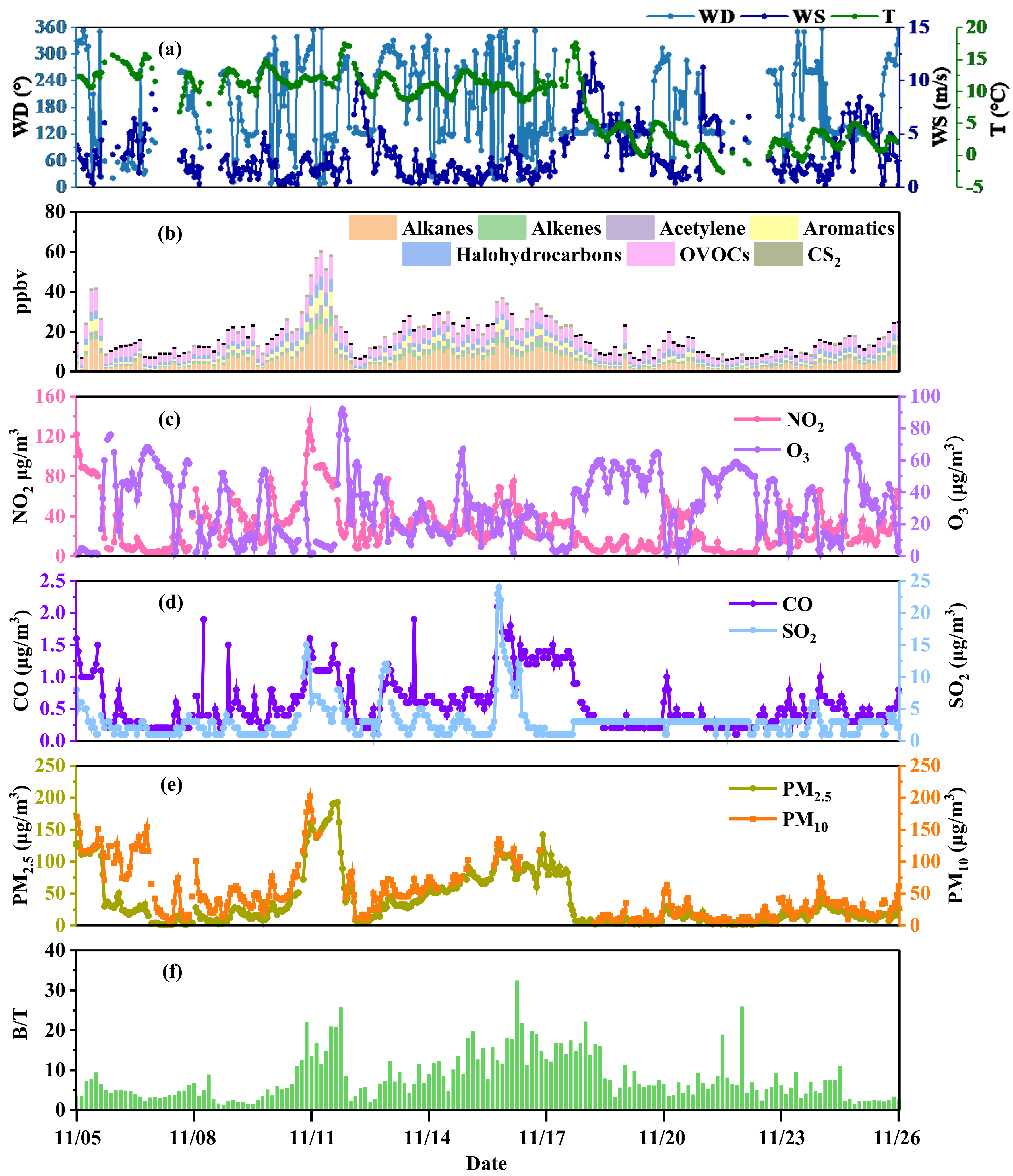
3.1. Overview of Meteorological Parameters and Air Quality

The hourly variation of meteorological parameters and air pollutants from 5–26 November 2020 is shown in Figure 1. During the sampling period, the mean values of T and WS were 10.66 °C and 3.03 m/s, respectively. As shown in the wind rose diagram in Figure S2, the dominant WDs during P1 were westerly and southeasterly, and the WD during P2 was mainly southeasterly. Additionally, the WS in P2 (3.39 ± 2.65 m/s) was significantly higher than that in P1 (2.58 ± 1.97 m/s). The average concentrations of NO2, O3, CO, and SO2 were 30.09 ± 23.27 μg/m3, 30.52 ± 20.27 μg/m3, 0.58 ± 0.40 mg/m3, and 3.04 ± 2.81 μg/m3, respectively. The average concentrations of PM2.5 and PM10 were 37.26 ± 41.06 μg/m3 and 47.61 ± 40.77 μg/m3, respectively. The concentration of TVOCs ranged from 5.85 to 60.19 ppbv, with an average value of 17.60 ± 10.25 ppbv.
During the whole campaign, the Pearson correlation coefficient between TVOCs and PM2.5 was the highest (r = 0.83, p < 0.01), indicating that they may have the same sources. In addition, TVOCs were positively correlated with PM10, NO2, CO, and SO2, and their correlation coefficients were 0.64, 0.68, 0.66 and 0.33 (p < 0.01), respectively. Furthermore, this study used trimethylbenzene (1,2,3-trimethylbenzene, 1,2,4-trimethylbenzene, 1,3,5-trimethylbenzene) and benzene, which have a 30-fold difference in OH reaction rate and similar sources, to evaluate the air aging level. As shown in Figure 1e, the ratio of benzene and trimethylbenzene (B/T ratio) was positively correlated with TVOCs (r = 0.44, p < 0.01) and higher in heavily polluted weather, indicating that the consumption of trimethylbenzene was higher than that of benzene under regional transmission. TVOCs were negatively correlated with wind speed, indicating that stagnant weather with low wind speed was more conducive to accumulation of VOCs. The RO2 generated by VOCs can oxidize NO to NO2, thereby reducing the consumption of NO to O3 and finally increasing the O3 concentration [38,39]. However, O3 was negatively correlated with TVOCs and NO2 in this study, and the occurrence of the peak concentration of O3 was about 12 h later than that of the peak concentrations of TVOCs and NO2. This phenomenon might be due to heavy-pollution weather increasing NO concentration and maintaining a NO–O3–NO2 dynamic equilibrium.
The diurnal variations in VOC groups, PM2.5, NO2, O3, and meteorological parameters are shown in Figure S3. The diurnal variations of alkanes, alkenes, acetylene, and aromatics were similar, with the lowest concentrations at 11:00–14:00 and higher concentrations at 7:00 and 19:00, which symbolized the bimodal features of vehicle emissions. Their diurnal variation was similar to that of NO2 and PM2.5, but completely opposite to that of O3, because stronger solar radiation and higher temperatures at noon promoted photochemical reaction. OVOCs had higher concentrations at noon as well and had another peak at 4:00 due to heavy pollution at night. Moreover, atmospheric pollutants could be easier to diffuse under the conditions of higher wind speed and atmospheric boundary layer at 7:00–16:00.

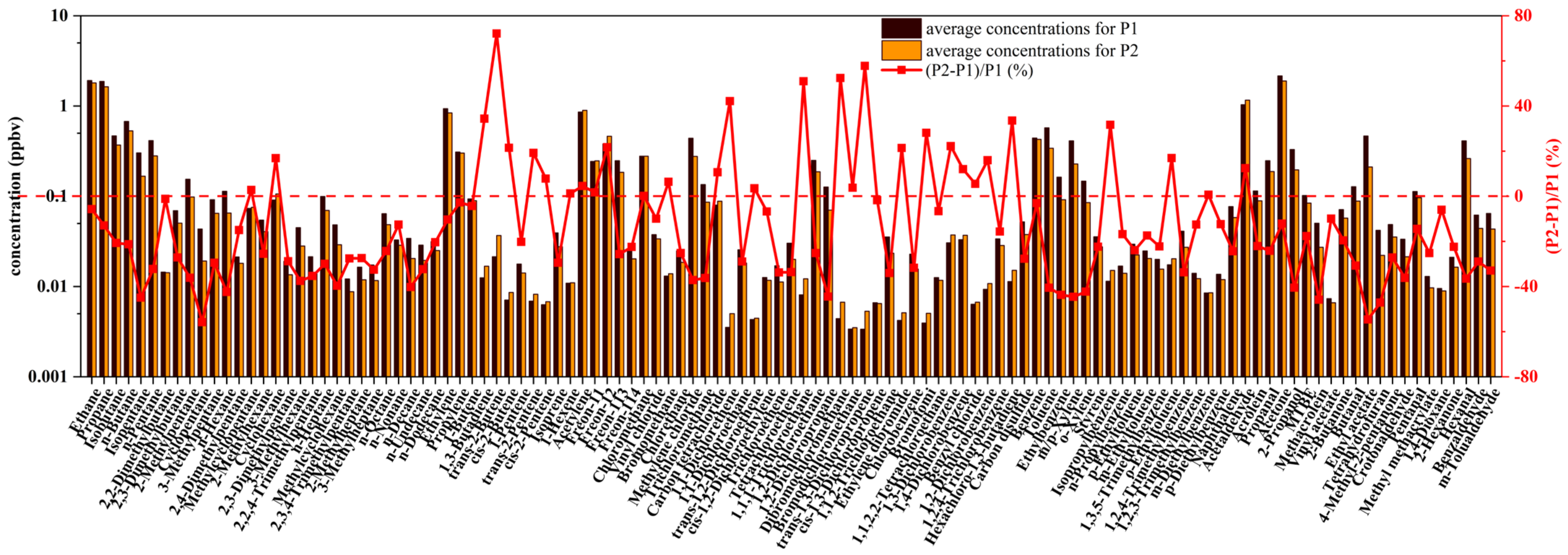
3.2. Concentrations and Compositions of VOCs
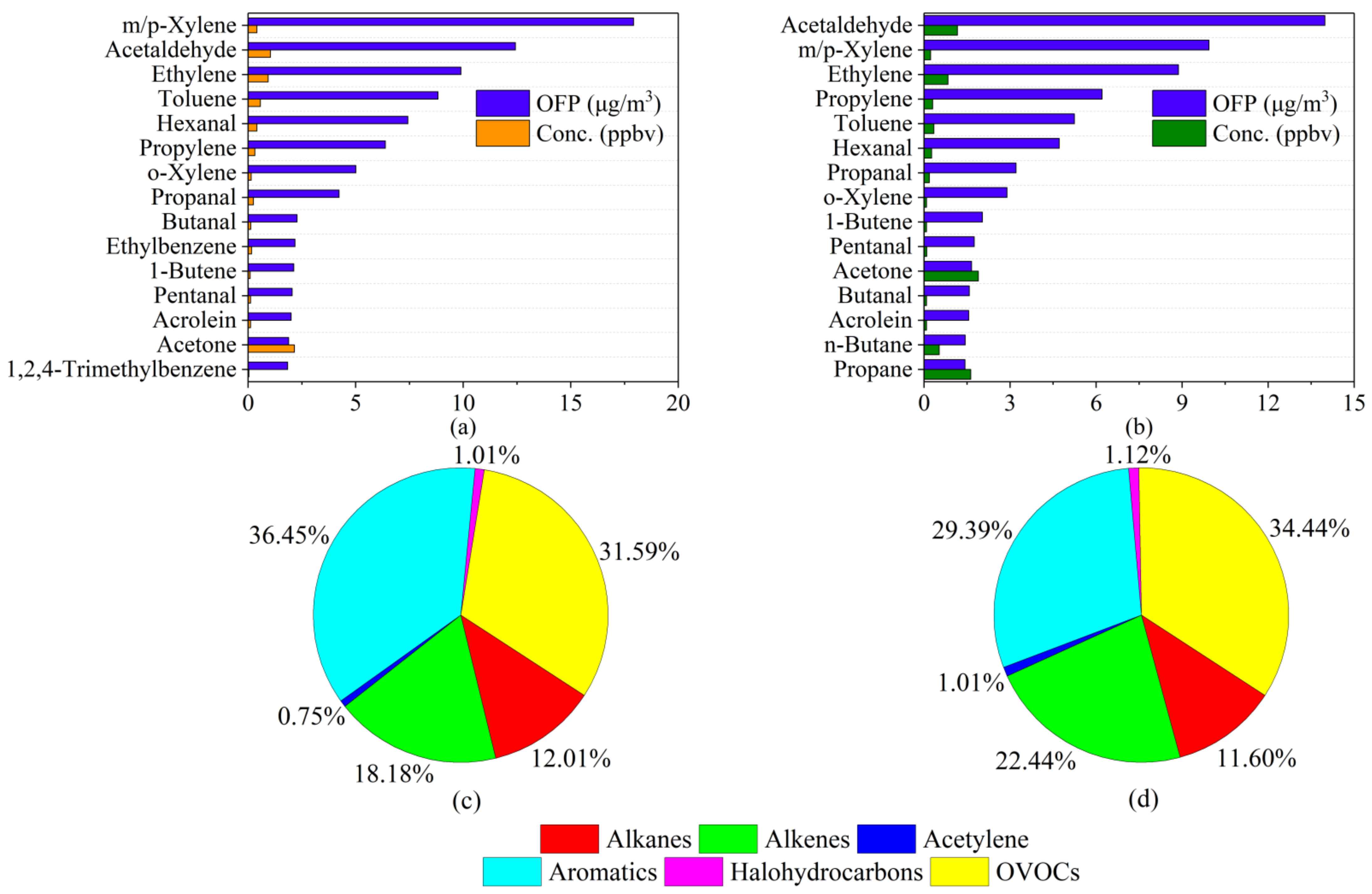
The descriptive statistical results for 116 VOC species during different periods are summarized in Table S6. The averaged TVOCs concentration in P1 was 19.43 ± 12.41 ppbv, higher than that in P2 (16.25 ± 8.01 ppbv). Figure 2 shows average concentrations of VOC groups, their compositions, and their relative differences between P1 and P2. Most alkanes, aromatics, and OVOC species were more abundant during P1 than P2, and their relative differences were 17.21%, 30.26%, and 17.40%, respectively. The concentration of acetylene in P2 was 4.52% higher than that in P1, which may be related to scattered coal burning in the heating period. The concentrations of alkenes with high reactivity and halohydrocarbons representing background sources were similar in P1 and P2. These results indicated that the relative differences between P1 and P2 were impacted mainly by aged and regional air mass transport.

3.3. OFP of VOCs

The average OFP value during P1 was 119.49 μg/m3, which was significantly higher than that during P2 (92.63 μg/m3). The top fifteen OFPs of VOC species during P1 and P2 are shown in Figure 3a,b. During P1, m/p-Xylene had the largest OFP value and contributed 17.92 μg/m3 OFP at a concentration of 0.41 ppbv, while during P2, acetaldehyde had the highest OFP value (13.98 μg/m3) at a concentration of 1.16 ppbv.
The contributions of VOC groups to the total OFP during P1 are shown in Figure 3c. Aromatics contributed most to the OFP (36.45%, 43.54 μg/m3), followed by OVOCs (31.59%, 37.74 μg/m3) and alkenes (18.18%, 21.72 μg/m3). As shown in Figure 3d, the OFP contribution of each group in P2 was different. The OFP value of OVOCs was the largest (34.44%, 31.89 μg/m3), followed by those of aromatics (29.39%, 27.22 μg/m3) and alkenes (22.44%, 20.78 μg/m3). This result indicates that vehicle exhaust and solvent usage played a dominant role in OFP during P1, while plant emissions and secondary generation contributed more to OFP during P2 [40,41]. Controlling emissions of related sources is an effective measure to reduce near-surface O3 pollution in the suburbs of Beijing. Although alkanes were dominant in terms of concentration (35.32%), their contribution to OFP was only nearly 12.01%, indicating that alkanes were not significant species for O3 formation. The contributions of acetylene and halohydrocarbons to OFP were almost negligible.

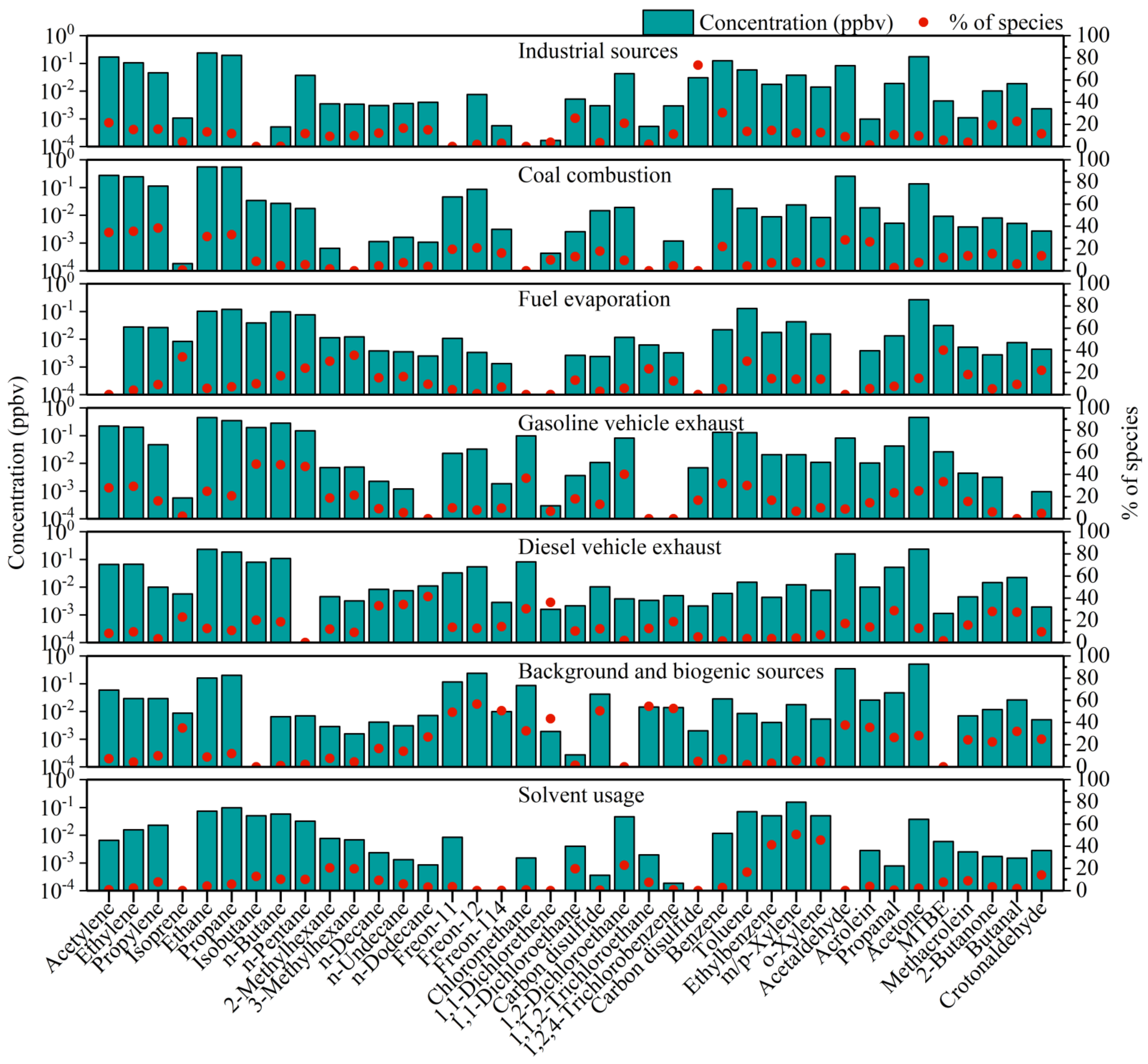
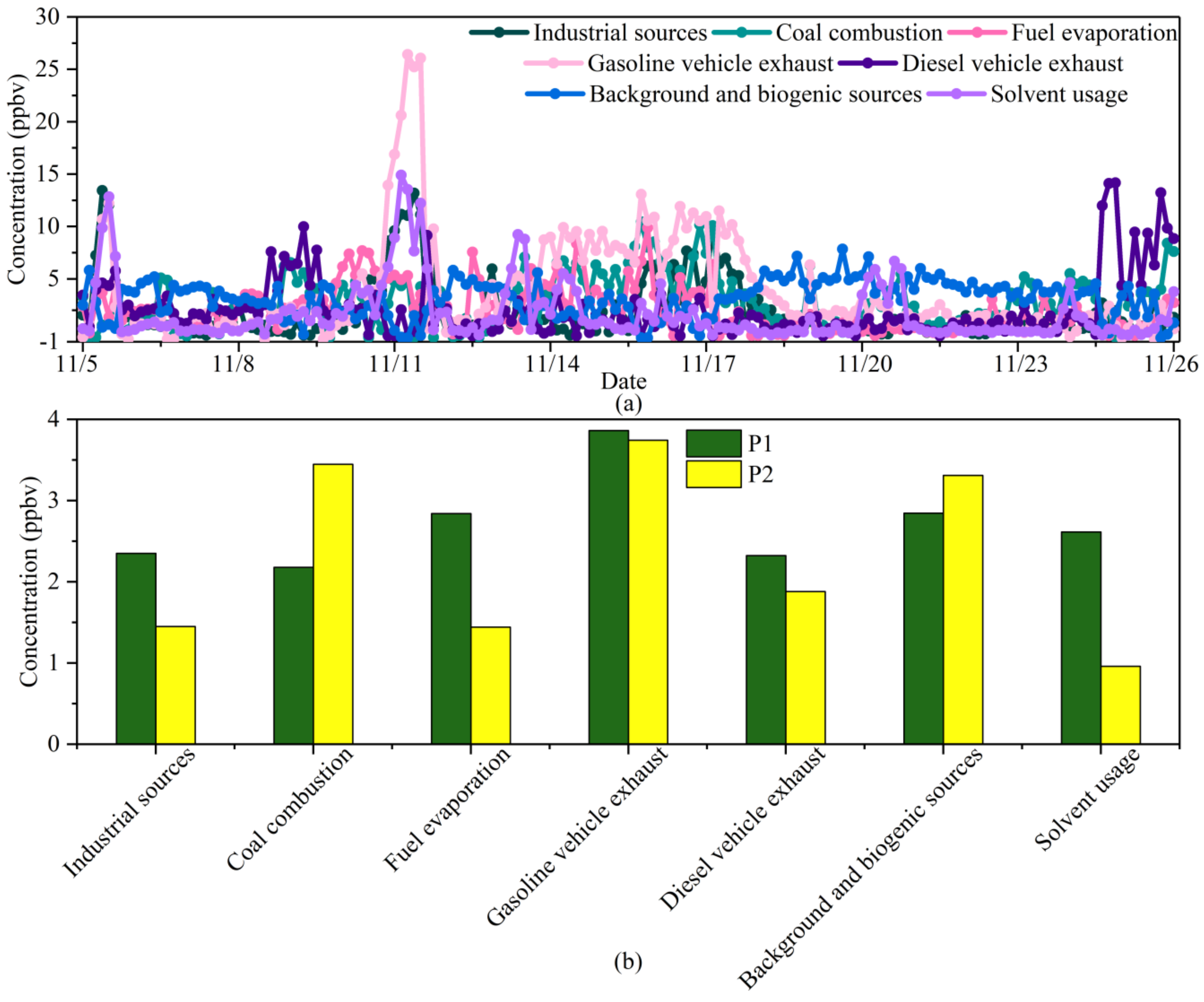
3.4. Source Apportionment

In the running of the PMF model, numbers of factors ranging from 4 to 10 were evaluated to determine the optimum solution. The variation of Q value with number of factors is shown in Figure S4. When the factor number was 7 to 10, Q(True)/Q(Robust) converged to 1.09. Theoretically, when the ratio of Q(true)/Q(robust) tends to 1, the impact of data points with high-scaled residuals is least. Based on the physical plausibility of the resulting profiles and residual distributions, the use of seven factors was determined to be the optimal solution. Values of Fpeak ranging from −1 to 1 at intervals of 0.2 were used in the model. An Fpeak of −0.2 was determined to be the optimum solution, and source profiles of the resolved factors are shown in Figure 4.
Factor 1 was identified as industrial sources, characterized by high percentages (73.46%) of CS2, which is mainly used in the production of viscose, rubber, and rayon [42,43]. This factor also had high contributions to 1,1-dichloroethane (25.52%), 1,2-dichloroethane (20.94%), and benzene (30.38%). Such high loadings of halohydrocarbons and aromatics were caused by industrial emissions [44,45]. 2-butanone is used as solvent in the manufacturing industry, and aldehyde is the main pollutant generated by the paint and textile furniture manufacturing industry [46,47]. This result was in good agreement with the contribution of factor 1 to butanal (22.67%) and 2-butanone (19.35%).
Factor 2 was attributed to coal combustion. Factor 2 had high contributions to acetylene (34.20%), ethylene (35.40%), propylene (38.05%), ethane (30.66%), propane (32.17%), and benzene (21.33%). VOCs emitted from coal combustion were mainly acetylene, C2–C3 alkenes, and C2–C3 alkanes [48]. Benzene was also a typical species released from the burning of fossil fuels [49].
Factor 3 was classified as fuel evaporation, characterized by high percentages of n-butane (17.00%), n-pentane (23.92%), 2-methylhexane (30.15%), and 3-methylhexane (35.44%). N-butane and n-pentane are the main tracers of gasoline volatilization [45,50]. Methyl tert-butyl ether (MTBE) is a commonly used gasoline additive, and this factor contributed 40.12% to it [51].
Factor 4 was identified as gasoline vehicle exhaust, characterized by high percentages of C2–C5 alkanes such as ethane (24.83%), propane (20.162%), isobutane (49.24%), n-butane (48.70%), and n-pentane (47.03%) [52]. Factor 4 contributed aromatic hydrocarbons such as benzene (31.77%), toluene (29.97%) and ethylbenzene (16.73%), which can also be attributed to gasoline usage [53]. MTBE (33.37%) is a commonly used additive to improve gasoline octane number, which was also reflected in this factor [54]. 1,2-dichloroethane (40.03%), as a petroleum hydrocarbon pollutant, was also contributed in a high percentage [55,56].
Factor 5 was identified as diesel vehicle exhaust. This factor had great contributions to n-decane (33.23%), n-undecane (34.26%), and n-dodecane (41.46%), which are the main products of diesel emissions [57]. In addition, this source also contributed to chloromethane (30.49%) and 1,1-dichloroethane (36.20%).
Factor 6 was characterized by high percentages of halohydrocarbons such as Freon-11 (49.29%), Freon-12 (56.76%), Freon-114 (50.28%), methyl chloride (32.36%), tetrachloromethane (50.40%), 1,1,2-trichloroethane (54.56%), and 1,2,4-trichlorobenzene (52.67%). These long-lifespan species can be regarded as tracers of background sources [58,59]. This factor contributed 35.08% to isoprene, which is an indicator of plant emission [60]. Isoprene can react with NO3, OH, and O3 in the atmosphere to produce aldehydes and ketones rapidly [61,62,63]. This factor also contributed to the oxidation products of isoprene such as acetaldehyde (37.63%), acrolein (35.54%), propanal (26.41%), acetone (28.06%), methacrolein (24.31%), 2-butanone (22.48%), butenal (31.93%), and crotonaldehyde (24.95%). Therefore, factor 6 was classified as background and biogenic sources.
Factor 7 possessed the property of high content of aromatics such as ethylbenzene (41.25%), m/p-xylene (50.67%), o-xylene (45.62%), and toluene (16.60%). The high ratio of aromatics was related to solvent usage in the adhesive, furniture, and shoemaking industries [40]. Additionally, 1,1-dichloroethane (19.78%) and 1,2-dichloroethane (22.86%) are commonly used as industrial adhesives in furniture, varnish, and paint stripper [64]. Hence, factor 7 was attributed to solvent usage.The time series of the seven factors, as well as their contribution percentages, are shown in Figure 5. Temporal variation in the concentration contribution of each source is shown in Figure 5a. All sources except for background and biogenic sources and diesel vehicle exhaust had peaks on 11 November, which were caused by persistent southern winds with low WS and temperature inversions. The contribution peaks of industrial sources and organic solvents appeared on several severely polluted days, and their Pearson correlation coefficient was 0.58, indicating that the two sources could be attributed to regional transport. In addition, the contribution peaks of fuel evaporation and gasoline vehicle exhaust occurred simultaneously, indicating that both factors were affected by traffic conditions. The contribution peak of diesel vehicle exhaust usually appeared at night, because trucks were allowed to enter downtown Beijing only at 23:00–6:00. The coal source had a high concentration after 14 November, in accordance with heating time. The background source contribution was relatively stable, with the smallest standard deviation, at 0.54, among all the sources (the average contribution of each source was set to 1).
Figure 5b shows that the average concentrations of sources during P1 and P2 were significantly different. The contribution of coal combustion during P2 increased significantly, accounting for 21.23% (3.45 ppbv) compared with only 11.46% (2.18 ppbv) during P1. This indicated that scattered coal might still be used in suburbs around Beijing. Contrarily, the relative contributions of industrial sources, fuel evaporation, and solvent usage all decreased more than 35% from P1 to P2. The contributions of background and biogenic sources and gasoline and diesel vehicle exhaust between P1 and P2 had no significant differences, indicating that heating activities had little impact on plant photosynthesis and traffic conditions.

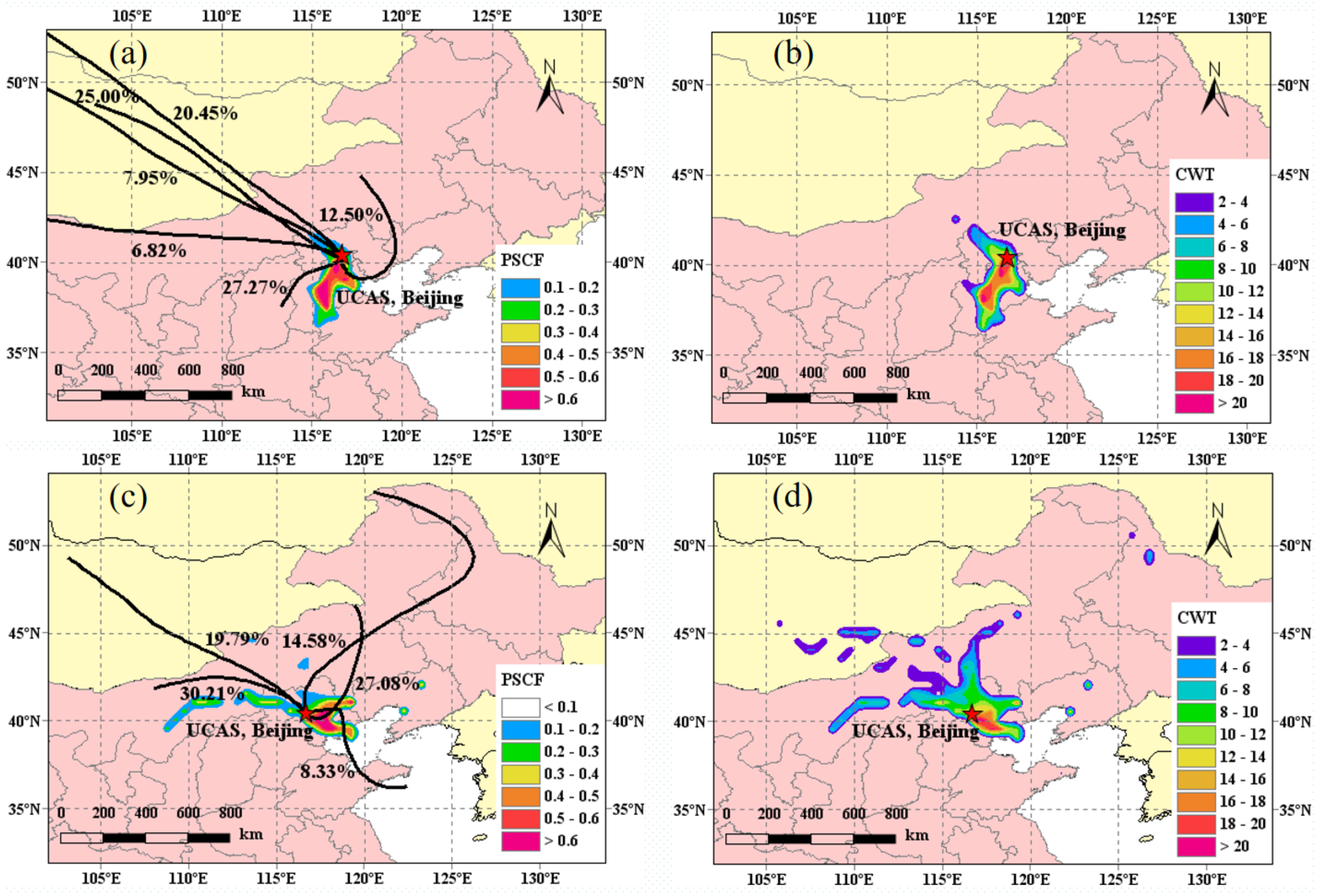
3.5. PSCF and CWT Results

As shown in Figure 6a, the northwest long-distance transport from Russia, Mongolia, and the Inner Mongolia Autonomous Region contributed 60.22% to Beijing’s air mass during P1. Contributions from short-distance transport from the southwest and medium-distance transport from the northeast were relatively small, amounting to 27.27% and 12.50%, respectively. From the results of PSCF, the regions that featured high PSCF values were concentrated mainly in southern Hebei Province and Tianjin. Based on the CWT results in Figure 6b, the strong sources of VOCs during P1 were mainly Baoding, Hebei Province, and local sources in Beijing.
As shown in Figure 6c, during P2, the main air mass came from the medium-distance transport from the western (30.21%) and northern Inner Mongolia Autonomous Region (27.08%), followed by long-distance transport from Mongolia (19.79%), Heilongjiang Province (14.58%), and medium-distance transport from Shandong Province (8.33%). The area with high PSCF value in P2 was smaller than that in P1, mainly in Beijing, northern Hebei Province, and Tianjin. As presented in Figure 6d, areas with CWT > 20 were located mainly in urban Beijing.
To the west of Beijing are the Taihang Mountains. The north and northeast are surrounded by the Yanshan Mountains, and the southern provinces of Hebei, Henan, and Shandong have many industrial enterprises [65]. It is easy for Beijing to accumulate air pollutants in the south wind and stagnant weather conditions, which was the main reason for the serious VOC pollution during P1. Nevertheless, air masses were mainly from the northwest. Therefore, the TVOCs concentration during P2 was lower than that during P1, although the contribution of coal combustion increased during the heating period.

3.6. Health Risk Assessment

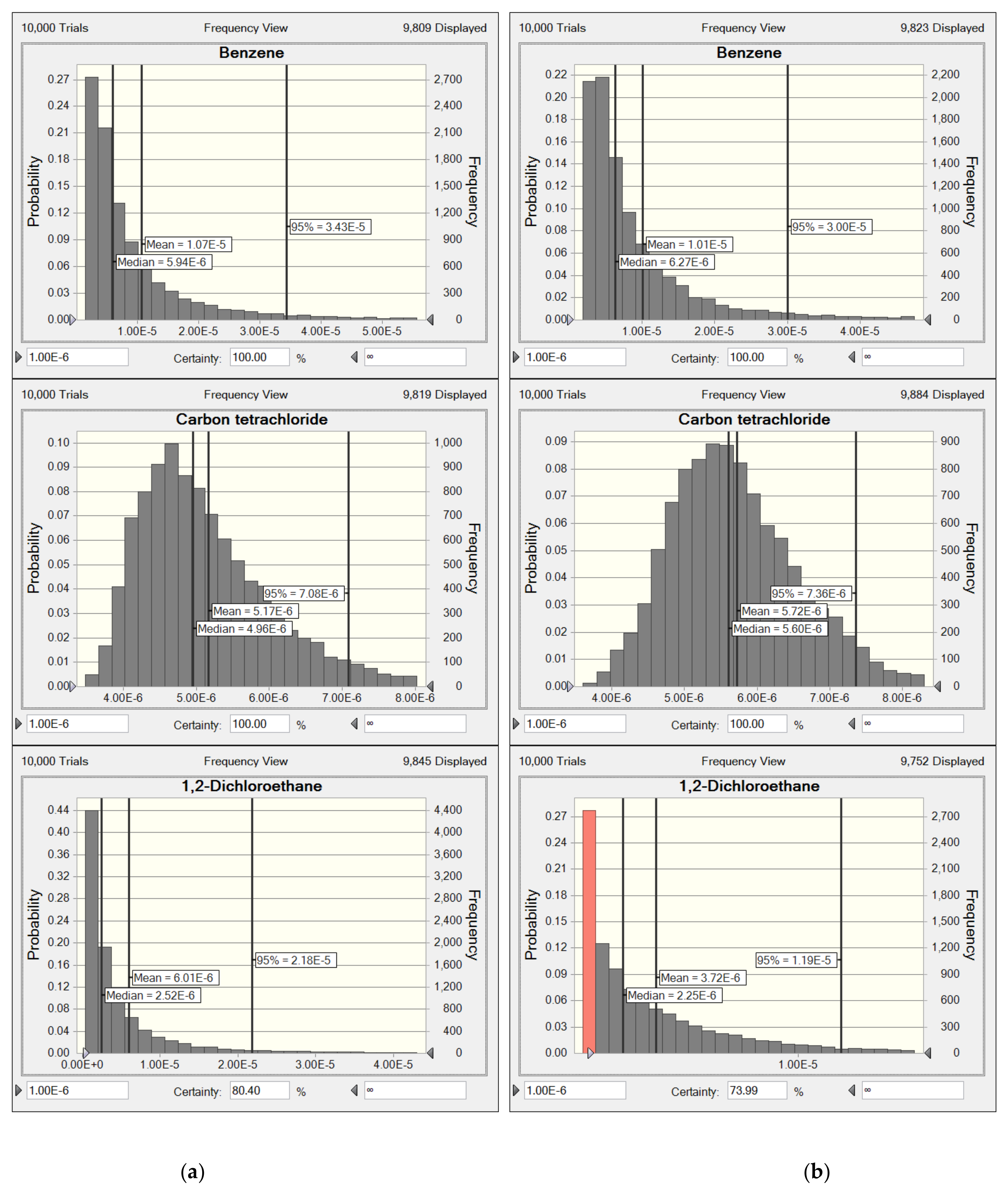
3.6.1. Noncarcinogenic and Carcinogenic Risks of VOC Species

The mean values of HQ of the 29 selected VOC species were all <1 during both periods. As shown in Figure S5, acrolein, benzene, and tetrachloromethane had relatively high HQ values during P1 and P2. The HI was calculated by summing the HQ values of VOC species affecting the same target organ (Table S7). The respiratory system had the highest HI values during P1 and P2, which were 0.83 and 0.65, respectively. Nevertheless, the HI values of all target organ systems were lower than 1, indicating that the chronic health risks caused by inhalation of selected VOCs in the suburbs of Beijing could be negligible.
For residential lifetime cancer risk assessment, the U.S. EPA divides the population into third trimester, infants (0–2), children (2–16), and adults (16–70). The normalized respiration rate of children was the highest after calculation, which was caused by the combined effect of respiration rate, body weight, and daily exposure time. Hence, the Monte Carlo simulation in this study used the correlation coefficient of children. As shown in Figure 7 and Figure 8 VOCs including benzene, tetrachloromethane, and 1,2-dichloroethane were higher than the U.S. EPA acceptable standard (1.0 × 10⁻⁶) during P1 and P2, and benzene was even higher than the stricter acceptable standard of the Canadian EPA (1.0 × 10⁻⁵) [66]. Furthermore, benzene and tetrachloromethane had high HQ values that might lead to noncarcinogenic hazards as well. Therefore, it is particularly important for suburban Beijing to control the VOC sources related to benzene and tetrachloromethane.

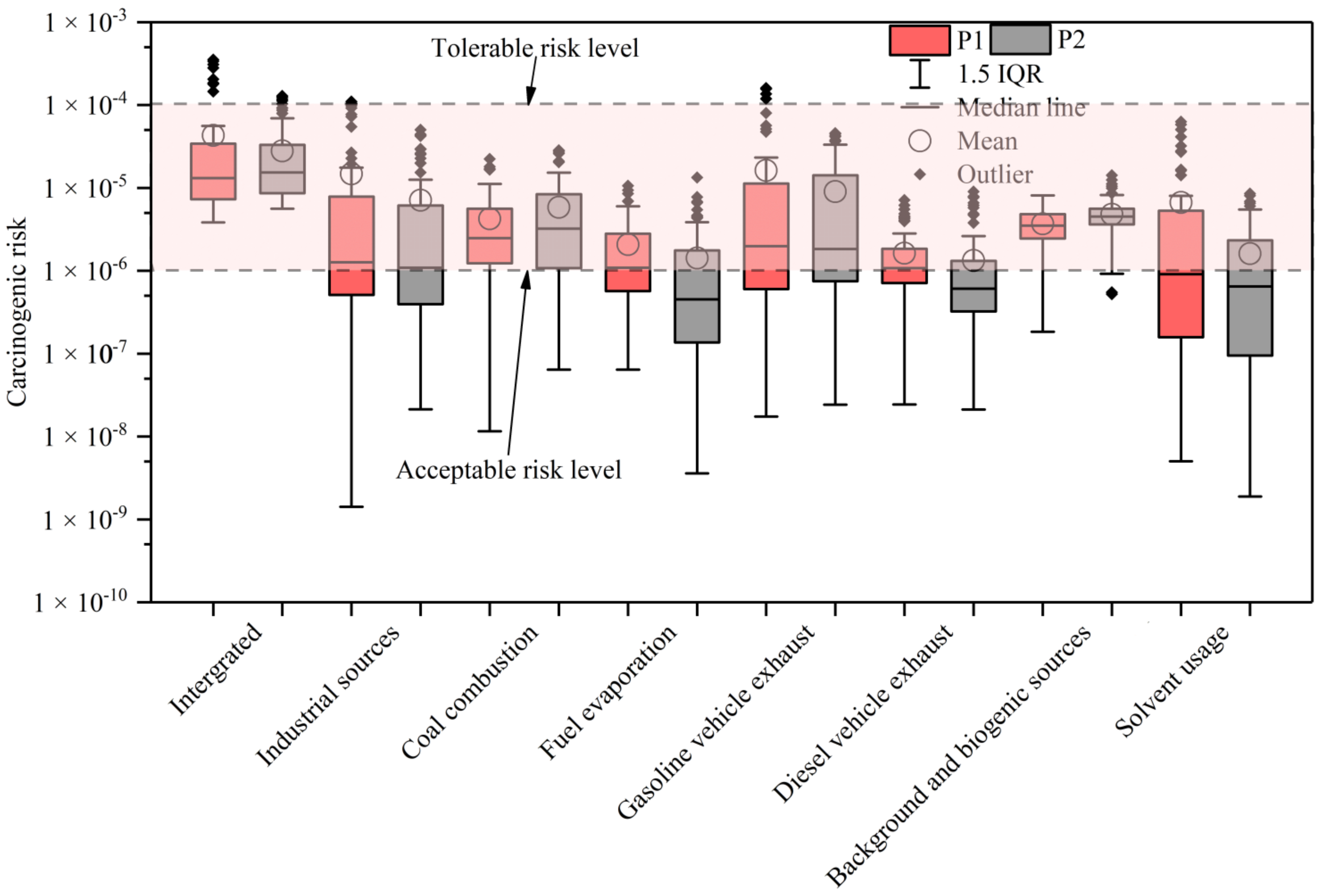
3.6.2. Carcinogenic Risks of VOC Sources

In order to propose more effective source control measures, we further calculated the carcinogenic risks of selected VOC species of PMF-derived sources by point estimation (Figure 8). The mean cancer risks of six sources ranged from 1.3 × 10⁻⁶ (diesel vehicle exhaust during P2) to 1.40 × 10⁻⁵ (gasoline during P1). The integrated carcinogenic risks during P1 and P2 were 4.30 × 10⁻⁵ and 2.80 × 10⁻⁵, which were below the U.S. EPA tolerable risk level (1.0 × 10⁻⁴). Out of six PMF-derived sources, gasoline vehicle exhaust, industrial source, and coal combustion exhibited higher risk values during both periods due to their high contributions to benzene or 1,2-dichloroethane. This was inconsistent with the finding that background sources had the highest cancer risks in some cities in Canada, which may be related to the local industrial structure [57,67]. In short, for public health, gasoline vehicle emissions, industrial enterprises, and coal combustion need more effective raw material pretreatment and emission control. Considering the regional transmission of VOCs, not only suburban Beijing but the surrounding provinces need to have corresponding control measures.

4. Conclusions

To assess the impact of heating on pollution characteristics and sources and health assessment in regard to VOCs, 116 VOC species were continuously monitored at UCAS, Beijing during 5–26 November 2020. The averaged TVOCs concentration during P1 was 19.43 ± 12.41 ppbv, higher than that (16.25 ± 8.01 ppbv) during P2. Most alkanes, aromatics, and OVOC species gave higher contributions during P1 than P2, and the concentrations of alkenes and halohydrocarbons were close during P1 and P2 because of the aged and regional air masses. The concentration of acetylene in P2 was 4.52% higher than that in P1, which may be related to scattered coal burning during the heating period.
During the whole sampling campaign, the concentration of TVOCs was positively correlated with the concentrations of PM2.5, PM10, NO2, CO, and SO2. However, O3 was negatively correlated with TVOCs and NO2 in this study, and the peak concentration of O3 was about 12 h later than those of TVOCs and NO2. Alkanes contributed most to the VOC mixing ratio during both P1 and P2, while aromatics and OVOCs contributed most to the OFP, with contributions of 36.44% and 34.43% during P1 and P2, respectively. These results indicate that vehicle exhaust and solvent usage were the main sources of the precursors of ozone, while the plant emissions and secondary generation contributed more OFP during P2. Controlling VOC and NOx emissions of gasoline vehicle exhaust, solvent usage, and industrial enterprises would constitute an effective measure to reduce near-surface O3 pollution in the suburbs of Beijing.
The 48 h backward trajectories, PSCF, and CWT showed that the air quality of Beijing during P1 was affected mainly by short-distance transportation from the southern Hebei Province. VOC pollution in Beijing was basically caused by local source emissions during P2, so the TVOCs concentration during P2 was lower than that during P1. After CTEP, although heating still contributed to VOCs in the suburbs of Beijing, the main cause of VOC heavy pollution events was regional transmission. Therefore, regional joint prevention and control of the 2 + 26 cities in North China is vital to Beijing’s air quality.
The seven sources identified from the PMF model were industrial source, coal combustion, fuel evaporation, gasoline vehicle exhaust, diesel vehicle exhaust, background and biogenic sources, and solvent usage. The contribution of coal combustion increased significantly during P2, indicating that scattered coal burning should be strictly controlled in suburban Beijing. Industrial sources, fuel evaporation, and solvent usage exhibited the opposite trend because of the regional transmission from southern Hebei Province during P1. Background and biogenic sources and gasoline and diesel vehicle exhaust showed no significant variation. Regarding the health risk assessment, the chronic noncarcinogenic risks of all selected VOC species were within the safe range, while the carcinogenic risks of most selected VOCs were above the acceptable risk level. From the perspective of public health, the cancer risks posed by gasoline vehicle emissions, industrial enterprises, and coal combustion should be paid more attention.

Supplementary Materials

The following supporting information can be downloaded at: https://www.mdpi.com/article/10.3390/atmos13040560/s1, Table S1. List of MDL, R2 and RSD of VOCs species; Table S2. Summary of PMF input data. Concentration units in ppbv; Table S3. The reference exposure level (REL) and cancer potency factor (CPF) of selected VOC species; Table S4. The target organ systems affected by non-carcinogenic adverse effects of selected VOC species; Table S5. Exposure parameters for calculating residential inhalation cancer risk for each age group; Table S6. Statistics of VOCs species during P1 and P2; Table S7. Substance-specific chronic inhalation hazard quotients (HQs) and the hazard index (HI) by target organ system during P1 and P2; Figure S1. Location of the sampling site in UCAS, Beijing; Figure S2. Wind rose diagrams during (a) P1 and (b) P2; Figure S3. Diurnal variations of VOC groups, PM2.5, NO2, O3 and meteorological parameters (T, WD and WS) during P1 and P2; Figure S4. Variation of Q Value with Factor in PMF Model; Figure S5. Probability distribution of HQ of selected VOC species during (a) P1 and (b) P2.

Author Contributions

Conceptualization, B.Z. and Y.Z. (Yang Zhang); methodology, B.Z. and P.H.; software, B.Z. and T.Z.; validation, T.Z. and L.Z.; formal analysis, B.Z.; investigation, B.Z. and Y.Z. (Yang Zhang); resources, Y.Z. (Yang Zhang) and Y.Z. (Yuanxun Zhang); data curation, J.M.; writing—original draft preparation, B.Z.; writing—review and editing, B.Z., T.Z. and Y.Z. (Yang Zhang); visualization, B.Z. and P.H.; supervision, Y.Z. (Yang Zhang) and Y.Z. (Yuanxun Zhang); project administration, Y.Z. (Yang Zhang) and Y.Z. (Yuanxun Zhang); funding acquisition, Y.Z. (Yang Zhang). All authors have read and agreed to the published version of the manuscript.

Funding

This research was funded by Fundamental Research Funds for the Central Universities (E0E48927X2) and the National Natural Science Foundation of China (21677145). And The APC was funded by [E0E48927X2].

Institutional Review Board Statement

Not applicable.

Informed Consent Statement

Not applicable.

Data Availability Statement

The concentrations of NO2, O3, CO, SO2, PM2.5, and PM10 were published by the Beijing Municiple Ecological and Environmental Monitoring Center and obtained from https://quotsoft.net/air/ (accessed on 1 July 2021). The meteorological parameters (temperature (T), wind speed (WS), and wind direction (WD)) were provided by Beijing Yanshan Earth Critical Zone National Research Station.

Conflicts of Interest

The authors declare no conflict of interest.

References

  1. Jiang, M.; Zou, L.; Li, X.-Q.; Che, F.; Zhao, G.-H.; Li, G.; Zhang, G.-N. Definition and Control Indicators of Volatile Organic Compounds in China. Huanjing Kexue 2015, 36, 3522–3532. [Google Scholar]
  2. Tai, X.H.; Chook, S.W.; Lai, C.W.; Lee, K.M.; Yang, T.C.K.; Chong, S.; Juan, J.C. Effective photoreduction of graphene oxide for photodegradation of volatile organic compounds. RSC Adv. 2019, 9, 18076–18086. [Google Scholar] [CrossRef] [Green Version]
  3. Jang, M.S.; Czoschke, N.M.; Lee, S.; Kamens, R.M. Heterogeneous atmospheric aerosol production by acid-catalyzed particle-phase reactions. Science 2002, 298, 814–817. [Google Scholar] [CrossRef]
  4. Sommariva, R.; de Gouw, J.A.; Trainer, M.; Atlas, E.; Goldan, P.D.; Kuster, W.C.; Warneke, C.; Fehsenfeld, F.C. Emissions and photochemistry of oxygenated VOCs in urban plumes in the Northeastern United States. Atmos. Chem. Phys. 2011, 11, 7081–7096. [Google Scholar] [CrossRef] [Green Version]
  5. Cooper, O.R.; Parrish, D.D.; Stohl, A.; Trainer, M.; Nedelec, P.; Thouret, V.; Cammas, J.P.; Oltmans, S.J.; Johnson, B.J.; Tarasick, D.; et al. Increasing springtime ozone mixing ratios in the free troposphere over western North America. Nature 2010, 463, 344–348. [Google Scholar] [CrossRef]
  6. Song, M.; Tan, Q.; Feng, M.; Qu, Y.; Liu, X.; An, J.; Zhang, Y. Source Apportionment and Secondary Transformation of Atmospheric Nonmethane Hydrocarbons in Chengdu, Southwest China. J. Geophys. Res. Atmos. 2018, 123, 9741–9763. [Google Scholar] [CrossRef]
  7. Zhou, J.; You, Y.; Bai, Z.; Hu, Y.; Zhang, J.; Zhang, N. Health risk assessment of personal inhalation exposure to volatile organic compounds in Tianjin, China. Sci. Total Environ. 2011, 409, 452–459. [Google Scholar] [CrossRef]
  8. Bolden, A.L.; Kwiatkowski, C.F.; Colborn, T. New Look at BTEX: Are Ambient Levels a Problem? Environ. Sci. Technol. 2015, 49, 11984–11989. [Google Scholar] [CrossRef]
  9. Li, Y.; Yin, S.; Yu, S.; Yuan, M.; Dong, Z.; Zhang, D.; Yang, L.; Zhang, R. Characteristics, source apportionment and health risks of ambient VOCs during high ozone period at an urban site in central plain, China. Chemosphere 2020, 250, 126283. [Google Scholar] [CrossRef]
  10. Emberson, L.D.; Pleijel, H.; Ainsworth, E.A.; van den Berg, M.; Ren, W.; Osborne, S.; Mills, G.; Pandey, D.; Dentener, F.; Buker, P.; et al. Ozone effects on crops and consideration in crop models. Eur. J. Agron. 2018, 100, 19–34. [Google Scholar] [CrossRef]
  11. Agyei, T.; Juran, S.; Edwards-Jonasova, M.; Fischer, M.; Svik, M.; Kominkova, K.; Ofori-Amanfo, K.K.; Marek, M.V.; Grace, J.; Urban, O. The Influence of Ozone on Net Ecosystem Production of a Ryegrass-Clover Mixture under Field Conditions. Atmosphere 2021, 12, 1629. [Google Scholar] [CrossRef]
  12. Gao, W.; Tang, G.; Xin, J.; Wang, L.; Wang, Y. Spatial-Temporal Variations of Ozone during Severe Photochemical Pollution over the Beijing-Tianjin-Hebei Region. Res. Environ. Sci. 2016, 29, 654–663. [Google Scholar]
  13. Zhang, C.; Liu, X.G.; Zhang, Y.Y.; Tan, Q.W.; Feng, M.; Qu, Y.; An, J.L.; Deng, Y.J.; Zhai, R.X.; Wang, Z.; et al. Characteristics, source apportionment and chemical conversions of VOCs based on a comprehensive summer observation experiment in Beijing. Atmos. Pollut. Res. 2021, 12, 183–194. [Google Scholar] [CrossRef]
  14. Zhang, L.H.; Wang, X.Z.; Li, H.; Cheng, N.L.; Zhang, Y.J.; Zhang, K.; Li, L. Variations in Levels and Sources of Atmospheric VOCs during the Continuous Haze and Non-Haze Episodes in the Urban Area of Beijing: A Case Study in Spring of 2019. Atmosphere 2021, 12, 171. [Google Scholar] [CrossRef]
  15. Zhan, J.; Feng, Z.; Liu, P.; He, X.; He, Z.; Chen, T.; Wang, Y.; He, H.; Mu, Y.; Liu, Y. Ozone and SOA formation potential based on photochemical loss of VOCs during the Beijing summer. Environ. Pollut. 2021, 285, 117444. [Google Scholar] [CrossRef]
  16. Zhang, H.; Ji, Y.; Wu, Z.; Peng, L.; Bao, J.; Peng, Z.; Li, H. Atmospheric volatile halogenated hydrocarbons in air pollution episodes in an urban area of Beijing: Characterization, health risk assessment and sources apportionment. Sci. Total Environ. 2022, 806, 150283. [Google Scholar] [CrossRef]
  17. Wang, M.; Shao, M.; Chen, W.; Yuan, B.; Lu, S.; Zhang, Q.; Zeng, L.; Wang, Q. A temporally and spatially resolved validation of emission inventories by measurements of ambient volatile organic compounds in Beijing, China. Atmos. Chem. Phys. 2014, 14, 5871–5891. [Google Scholar] [CrossRef] [Green Version]
  18. Wei, W.; Li, Y.; Wang, Y.; Cheng, S.; Wang, L. Characteristics of VOCs during haze and non-haze days in Beijing, China: Concentration, chemical degradation and regional transport impact. Atmos. Environ. 2018, 194, 134–145. [Google Scholar] [CrossRef]
  19. Li, J.; Hao, Y.; Simayi, M.; Shi, Y.; Xi, Z.; Xie, S. Verification of anthropogenic VOC emission inventory through ambient measurements and satellite retrievals. Atmos. Chem. Phys. 2019, 19, 5905–5921. [Google Scholar] [CrossRef] [Green Version]
  20. Cheng, M.; Zhi, G.; Tang, W.; Liu, S.; Dang, H.; Guo, Z.; Du, J.; Du, X.; Zhang, W.; Zhang, Y.; et al. Air pollutant emission from the underestimated households’ coal consumption source in China. Sci. Total Environ. 2017, 580, 641–650. [Google Scholar] [CrossRef]
  21. Peng, L.; Zhang, Q.; Yao, Z.; Mauzerall, D.L.; Kang, S.; Du, Z.; Zheng, Y.; Xue, T.; He, K. Underreported coal in statistics: A survey-based solid fuel consumption and emission inventory for the rural residential sector in China. Appl. Energy 2019, 235, 1169–1182. [Google Scholar] [CrossRef]
  22. Logan, J.A. Tropospheric ozone: Seasonal behavior, trends, and anthropogenic influence. J. Geophys. Res. Atmos. 1985, 90, 10463–10482. [Google Scholar] [CrossRef]
  23. Roelofs, G.J.; Lelieveld, J. Model study of the influence of cross-tropopause O3 transports on tropospheric O3 levels. Tellus B 1997, 49, 38–55. [Google Scholar] [CrossRef] [Green Version]
  24. Carter, W. Updated Maximum Incremental Reactivity Scale and Hydrocarbon Bin Reactivities for Regulatory Applications. California Air Resources Board Contract 07-339. 2010. Available online: https://www.researchgate.net/publication/284060890_Updated_maximum_incremental_reactivity_scale_and_hydrocarbon_bin_reactivities_for_regulatory_applications (accessed on 10 July 2021).
  25. Kuo, C.-P.; Liao, H.-T.; Chou, C.C.K.; Wu, C.-F. Source apportionment of particulate matter and selected volatile organic compounds with multiple time resolution data. Sci. Total Environ. 2014, 472, 880–887. [Google Scholar] [CrossRef]
  26. Tan, Y.; Han, S.; Chen, Y.; Zhang, Z.; Li, H.; Li, W.; Yuan, Q.; Li, X.; Wang, T.; Lee, S.-C. Characteristics and source apportionment of volatile organic compounds (VOCs) at a coastal site in Hong Kong. Sci. Total Environ. 2021, 777, 146241. [Google Scholar] [CrossRef]
  27. Gary Norris, R.D. EPA Positive Matrix Factorization (PMF) 5.0 Fundamentals and User Guide. U.S.; Environmental Protection Agency: San Francisco, CA, USA, 2014. Available online: https://nepis.epa.gov/Exe/ZyPURL.cgi?Dockey=P100IW74.txt (accessed on 20 July 2021).
  28. Guo, H.; Cheng, H.R.; Ling, Z.H.; Louie, P.K.K.; Ayoko, G.A. Which emission sources are responsible for the volatile organic compounds in the atmosphere of Pearl River Delta? J. Hazard. Mater. 2011, 188, 116–124. [Google Scholar] [CrossRef]
  29. Paatero, P.; Hopke, P.K.J.A.C.A. Discarding or Downweighting High-Noise Variables in Factor Analytic Models. Anal. Chim. Acta 2003, 490, 277–289. [Google Scholar] [CrossRef]
  30. Draxier, R.R.; Hess, G.D. An overview of the HYSPLIT_4 modelling system for trajectories, dispersion and deposition. Aust. Meteorol. Mag. 1998, 47, 295–308. [Google Scholar]
  31. Li, Q.Q.; Su, G.J.; Li, C.Q.; Liu, P.F.; Zhao, X.X.; Zhang, C.L.; Sun, X.; Mu, Y.J.; Wu, M.G.; Wang, Q.L.; et al. An investigation into the role of VOCs in SOA and ozone production in Beijing, China. Sci. Total Environ. 2020, 720, 14. [Google Scholar] [CrossRef]
  32. Polissar, A.V.; Hopke, P.K.; Paatero, P.; Kaufmann, Y.J.; Hall, D.K.; Bodhaine, B.A.; Dutton, E.G.; Harris, J.M. The aerosol at Barrow, Alaska: Long-term trends and source locations. Atmos. Environ. 1999, 33, 2441–2458. [Google Scholar] [CrossRef]
  33. Hsu, Y.K.; Holsen, T.M.; Hopke, P.K. Comparison of hybrid receptor models to locate PCB sources in Chicago. Atmos. Environ. 2003, 37, 545–562. [Google Scholar] [CrossRef]
  34. Han, Y.J.; Holsen, T.M.; Hopke, P.K.; Yi, S.M. Comparison between back-trajectory based modeling and Lagrangian backward dispersion Modeling for locating sources of reactive gaseous mercury. Environ. Sci. Technol. 2005, 39, 1715–1723. [Google Scholar] [CrossRef]
  35. Wang, Y.Q.; Zhang, X.Y.; Arimoto, R. The contribution from distant dust sources to the atmospheric particulate matter loadings at XiAn, China during spring. Sci. Total Environ. 2006, 368, 875–883. [Google Scholar] [CrossRef]
  36. Hsu, C.Y.; Chiang, H.C.; Shie, R.H.; Ku, C.H.; Lin, T.Y.; Chen, M.J.; Chen, N.T.; Chen, Y.C. Ambient VOCs in residential areas near a large-scale petrochemical complex: Spatiotemporal variation, source apportionment and health risk. Environ. Pollut. 2018, 240, 95–104. [Google Scholar] [CrossRef]
  37. CalEPA. Guidance Manual for Preparation of Health Risk Assessments. California, USA. 2015. Available online: http://citeseerx.ist.psu.edu/viewdoc/summary?doi=10.1.1.589.1068 (accessed on 25 July 2021).
  38. Hui, L.; Liu, X.; Tan, Q.; Feng, M.; An, J.; Qu, Y.; Zhang, Y.; Deng, Y.; Zhai, R.; Wang, Z. VOC characteristics, chemical reactivity and sources in urban Wuhan, central China. Atmos. Environ. 2020, 224, 117340. [Google Scholar] [CrossRef]
  39. Li, Y.; Gao, R.; Xue, L.; Wu, Z.; Yang, X.; Gao, J.; Ren, L.; Li, H.; Ren, Y.; Li, G.; et al. Ambient volatile organic compounds at Wudang Mountain in Central China: Characteristics, sources and implications to ozone formation. Atmos. Res. 2021, 250, 105359. [Google Scholar] [CrossRef]
  40. Liu, B.; Liang, D.; Yang, J.; Dai, Q.; Bi, X.; Feng, Y.; Yuan, J.; Xiao, Z.; Zhang, Y.; Xu, H. Characterization and source apportionment of volatile organic compounds based on 1-year of observational data in Tianjin, China. Environ. Pollut. 2016, 218, 757–769. [Google Scholar] [CrossRef]
  41. Wu, F.; Yu, Y.; Sun, J.; Zhang, J.; Wang, J.; Tang, G.; Wang, Y. Characteristics, source apportionment and reactivity of ambient volatile organic compounds at Dinghu Mountain in Guangdong Province, China. Sci. Total Environ. 2016, 548, 347–359. [Google Scholar] [CrossRef]
  42. Vermeulen, R.; Jonsson, B.A.G.; Lindh, C.H.; Kromhout, H. Biological monitoring of carbon disulphide and phthalate exposure in the contemporary rubber industry. Int. Arch. Occup. Environ. Health 2005, 78, 663–669. [Google Scholar] [CrossRef]
  43. Asaro, L.; Gratton, M.; Poirot, N.; Seghar, S.; Hocine, N.A. Devulcanization of natural rubber industry waste in supercritical carbon dioxide combined with diphenyl disulfide. Waste Manag. 2020, 118, 647–654. [Google Scholar] [CrossRef]
  44. Ling, Z.H.; Guo, H.; Cheng, H.R.; Yu, Y.F. Sources of ambient volatile organic compounds and their contributions to photochemical ozone formation at a site in the Pearl River Delta, southern China. Environ. Pollut. 2011, 159, 2310–2319. [Google Scholar] [CrossRef]
  45. Hui, L.; Liu, X.; Tan, Q.; Feng, M.; An, J.; Qu, Y.; Zhang, Y.; Jiang, M. Characteristics, source apportionment and contribution of VOCs to ozone formation in Wuhan, Central China. Atmos. Environ. 2018, 192, 55–71. [Google Scholar] [CrossRef]
  46. Legreid, G.; Loeoev, J.B.; Staehelin, J.; Hueglin, C.; Hill, M.; Buchmann, B.; Prevot, A.S.H.; Reimann, S. Oxygenated volatile organic compounds (OVOCs) at an urban background site in Zurich (Europe): Seasonal variation and source allocation. Atmos. Environ. 2007, 41, 8409–8423. [Google Scholar] [CrossRef]
  47. Liang, X.; Chen, X.; Zhang, J.; Shi, T.; Sun, X.; Fan, L.; Wang, L.; Ye, D. Reactivity-based industrial volatile organic compounds emission inventory and its implications for ozone control strategies in China. Atmos. Environ. 2017, 162, 115–126. [Google Scholar] [CrossRef]
  48. Li, G.; Wei, W.; Shao, X.; Nie, L.; Wang, H.; Yan, X.; Zhang, R. A comprehensive classification method for VOC emission sources to tackle air pollution based on VOC species reactivity and emission amounts. J. Environ. Sci. 2018, 67, 78–88. [Google Scholar] [CrossRef]
  49. Sarkar, C.; Sinha, V.; Kumar, V.; Rupakheti, M.; Panday, A.; Mahata, K.S.; Rupakheti, D.; Kathayat, B.; Lawrence, M.G. Overview of VOC emissions and chemistry from PTR-TOF-MS measurements during the SusKat-ABC campaign: High acetaldehyde, isoprene and isocyanic acid in wintertime air of the Kathmandu Valley. Atmos. Chem. Phys. 2016, 16, 3979–4003. [Google Scholar] [CrossRef] [Green Version]
  50. Wang, B.; Shao, M.; Lu, S.H.; Yuan, B.; Zhao, Y.; Wang, M.; Zhang, S.Q.; Wu, D. Variation of ambient non-methane hydrocarbons in Beijing city in summer 2008. Atmos. Chem. Phys. 2010, 10, 5911–5923. [Google Scholar] [CrossRef] [Green Version]
  51. Chang, C.-C.; Wang, J.-L.; Liu, S.-C.; Lung, S.-C.C. Assessment of vehicular and non-vehicular contributions to hydrocarbons using exclusive vehicular indicators. Atmos. Environ. 2006, 40, 6349–6361. [Google Scholar] [CrossRef]
  52. Chen, C.-H.; Chuang, Y.-C.; Hsieh, C.-C.; Lee, C.-S. VOC characteristics and source apportionment at a PAMS site near an industrial complex in central Taiwan. Atmos. Pollut. Res. 2019, 10, 1060–1074. [Google Scholar] [CrossRef]
  53. Bari, M.A.; Kindzierski, W.B.; Wheeler, A.J.; Heroux, M.-E.; Wallace, L.A. Source apportionment of indoor and outdoor volatile organic compounds at homes in Edmonton, Canada. Build. Environ. 2015, 90, 114–124. [Google Scholar] [CrossRef]
  54. Legreid, G.; Reimann, S.; Steinbacher, M.; Staehelin, J.; Young, D.; Stemmler, K. Measurements of OVOCs and NMHCs in a swiss highway tunnel for estimation of road transport emissions. Environ. Sci. Technol. 2007, 41, 7060–7066. [Google Scholar] [CrossRef] [PubMed]
  55. Zhang, X.; Ma, Z.; Guo, X.Y.; Lu, H. In Source Apportionment of Petroleum Hydrocarbon Contamination in Karst Fissure Groundwater. DEStech Transactions on Environment, Energy and Earth Science. 2017. Available online: https://www.researchgate.net/publication/318892903_Source_Apportionment_of_Petroleum_Hydrocarbon_Contamination_in_Karst_Fissure_Groundwater (accessed on 7 August 2021).
  56. Heibati, B.; Pollitt, K.J.G.; Charati, J.Y.; Ducatman, A.; Shokrzadeh, M.; Karimi, A.; Mohammadyan, M. Biomonitoring-based exposure assessment of benzene, toluene, ethylbenzene and xylene among workers at petroleum distribution facilities. Ecotoxicol. Environ. Saf. 2018, 149, 19–25. [Google Scholar] [CrossRef] [PubMed]
  57. Xiong, Y.; Bari, M.A.; Xing, Z.; Du, K. Ambient volatile organic compounds (VOCs) in two coastal cities in western Canada: Spatiotemporal variation, source apportionment, and health risk assessment. Sci. Total Environ. 2020, 706, 135970. [Google Scholar] [CrossRef] [PubMed]
  58. Han, Y.; Huang, X.F.; Wang, C.; Zhu, B.; He, L.Y. Characterizing oxygenated volatile organic compounds and their sources in rural atmospheres in China. J. Environ. Sci. 2019, 81, 148–155. [Google Scholar] [CrossRef]
  59. Zhang, F.; Shang, X.; Chen, H.; Xie, G.; Fu, Y.; Wu, D.; Sun, W.; Liu, P.; Zhang, C.; Mu, Y.; et al. Significant impact of coal combustion on VOCs emissions in winter in a North China rural site. Sci. Total Environ. 2020, 720, 137617. [Google Scholar] [CrossRef]
  60. Hui, L.; Liu, X.; Tan, Q.; Feng, M.; An, J.; Qu, Y.; Zhang, Y.; Cheng, N. VOC characteristics, sources and contributions to SOA formation during haze events in Wuhan, Central China. Sci. Total Environ. 2019, 650, 2624–2639. [Google Scholar] [CrossRef]
  61. Stroud, C.A.; Roberts, J.M.; Goldan, P.D.; Kuster, W.C.; Murphy, P.C.; Williams, E.J.; Hereid, D.; Parrish, D.; Sueper, D.; Trainer, M.; et al. Isoprene and its oxidation products, methacrolein and methylvinyl ketone, at an urban forested site during the 1999 Southern Oxidants Study. J. Geophys. Res. Atmos. 2001, 106, 8035–8046. [Google Scholar] [CrossRef] [Green Version]
  62. Xie, X.; Shao, M.; Liu, Y.; Lu, S.; Chang, C.-C.; Chen, Z.-M. Estimate of initial isoprene contribution to ozone formation potential in Beijing, China. Atmos. Environ. 2008, 42, 6000–6010. [Google Scholar] [CrossRef]
  63. Starn, T.K.; Shepson, P.B.; Bertman, S.B.; Riemer, D.D.; Zika, R.G.; Olszyna, K. Nighttime isoprene chemistry at an urban-impacted forest site. J. Geophys. Res. Atmos. 1998, 103, 22437–22447. [Google Scholar] [CrossRef]
  64. Cai, C.J.; Geng, F.H.; Tie, X.X.; Yu, Q.O.; An, J.L. Characteristics and source apportionment of VOCs measured in Shanghai, China. Atmos. Environ. 2010, 44, 5005–5014. [Google Scholar] [CrossRef]
  65. Liu, Y.; Song, M.; Liu, X.; Zhang, Y.; Hui, L.; Kong, L.; Zhang, Y.; Zhang, C.; Qu, Y.; An, J.; et al. Characterization and sources of volatile organic compounds (VOCs) and their related changes during ozone pollution days in 2016 in Beijing, China. Environ. Pollut. 2020, 257, 113599. [Google Scholar] [CrossRef]
  66. Canada, H. Federal Contaminated Site Risk Assessment in Canada Part I: Guidance on Human Health Preliminary Quantitative Risk Assessment. 2004. Available online: http://www.publications.gc.ca/collections/Collection/H46-2-04-367E.pdf (accessed on 5 November 2021).
  67. Bari, M.A.; Kindzierski, W.B. Ambient volatile organic compounds (VOCs) in Calgary, Alberta: Sources and screening health risk assessment. Sci. Total Environ. 2018, 631–632, 627–640. [Google Scholar] [CrossRef] [Green Version]
Figure 1. Hourly variations of meteorological parameters, PM2.5, PM10, and gaseous pollutants and variations of three-hour average concentrations of VOCs at UCAS, Beijing from 5–26 November 2020: (a) wind direction (WD), wind speed (WS), and temperature (T), (b) VOC concentration, (c) NO2 and O3 concentration, (d) CO and SO2 concentration, (e) PM2.5 and PM10 concentration, (f) B/T (benzene/trimethylbenzene) ratio.
Atmosphere 13 00560 g001
Figure 2. Average concentrations of VOC species during nonheating (P1) and heating (P2) periods and the relative differences between these two periods.
Atmosphere 13 00560 g002
Figure 3. The top 15 VOCs in terms of ozone formation potential (OFP) their concentrations during (a) P1 and (b) P2 and contributions of groups of VOCs to the total OFP during (c) P1 and (d) P2.
Atmosphere 13 00560 g003
Figure 4. Source profiles of the resolved factors from the positive matrix factorization (PMF) model.
Atmosphere 13 00560 g004
Figure 5. (a) Concentration time series and (b) average concentration of the PMF-resolved sources of VOCs during P1 and P2.
Atmosphere 13 00560 g005
Figure 6. The 48 h backward trajectories, potential source contribution function (PSCF), and concentration weighted trajectory (CWT) from Beijing during (a,b) P1 and (c,d) P2.
Atmosphere 13 00560 g006
Figure 7. Probability distribution of cancer risks of selected VOC species during (a) P1 and (b) P2.
Atmosphere 13 00560 g007
Figure 8. Carcinogenic risks of PMF-derived VOC sources.
Atmosphere 13 00560 g008
Publisher’s Note: MDPI stays neutral with regard to jurisdictional claims in published maps and institutional affiliations.

