Article

Crop Residue Burning Emissions and the Impact on Ambient Particulate Matters over South Korea

1
School of Earth Sciences and Environmental Engineering, Gwangju Institute of Science and Technology (GIST), Gwangju 61005, Korea
2
Center for Earth Environmental Modeling Studies (CEMOS), Gwangju Institute of Science and Technology (GIST), Gwangju 61005, Korea
3
Central Research Facilities, Gwangju Institute of Science and Technology (GIST), Gwangju 61005, Korea
4
Department of Environmental Engineering, Mokpo National University, Muan 58554, Korea
5
The Seoul Institute, Seoul 06756, Korea
6
Department of Health Management, Kyung-in Women’s University, Incheon 21041, Korea
*
Author to whom correspondence should be addressed.
Atmosphere 2022, 13(4), 559; https://doi.org/10.3390/atmos13040559
Submission received: 17 February 2022 / Revised: 23 March 2022 / Accepted: 29 March 2022 / Published: 30 March 2022
(This article belongs to the Special Issue Physical, Chemical and Optical Properties of Aerosols)

Abstract

:
In the study, crop residue burning (CRB) emissions were estimated based on field surveys and combustion experiments to assess the impact of the CRB on particulate matter over South Korea. The estimates of CRB emissions over South Korea are 9514, 8089, 4002, 2010, 172,407, 7675, 33, and 5053 Mg year−1 for PM10, PM2.5, OC, EC, CO, NOx, SO2, and NH3, respectively. Compared with another study, our estimates in the magnitudes of CRB emissions were not significantly different. When the CRB emissions are additionally considered in the simulation, the monthly mean differences in PM2.5 (i.e., △PM2.5) were marginal between 0.07 and 0.55 μg m−3 over South Korea. Those corresponded to 0.6–4.3% in relative differences. Additionally, the △PM10 was 0.07–0.60 μg m−3 over South Korea. In the spatial and temporal aspects, the increases in PM10 and PM2.5 were high in Gyeongbuk (GB) and Gyeongnam (GN) provinces in June, October, November, and December.

1. Introduction

The air quality in South Korea has been gradually improving over the past decades [1]. The recent concentrations of the particulate matter showed a rapid decline, in particular during the period of the coronavirus COVID-19 pandemic [2,3]. Nevertheless, there is still apprehension about serious air quality, and the annual average levels of PM10 and PM2.5 do not meet the WHO air quality guidelines [4]. The South Korean government planned to reduce the PM2.5 emissions by 35.8% by 2022 from 2014. To reduce the concentrations of particulate matter, the government has established policies (e.g., Special Act on Fine Aerosol) for each ministry and has implemented reduction measures as follows [3]:
-
In energy production, conversion from coal-fired power plants to liquefied natural gas (LNG)-fired plants (i.e., coal-to-gas switching).
-
In the industry section, extending the environmental management policy for total amount control of air pollutants from the Seoul Metropolitan area to the whole country.
-
In transportation, early scrappage of old diesel vehicles and supply of low-emission vehicles such as electric and hybrid vehicles.
In the agricultural section, the South Korean government also strengthened the enforcement actions against illegal open burning activities. Nevertheless, as agricultural practices, crop residue burning (CRB) activities have been conducted in the field after harvest to manage the large quantities of the crop residues and to provide some nutrients from the residues (e.g., ashes) into the soil [5,6]. However, there are few studies to quantify the CRB emission and examine their impacts on particulate matter in South Korea.
Similarly, the CRB has often occurred in China, India, Myanmar, Thailand, Laos, Cambodia, and Vietnam [7,8,9,10,11]. The emissions from crop residue burning (or biomass burning) activities are closely related to radiative effects, air pollution, and public health [12,13,14,15]. Crutzen and Andreae reported that gaseous species of CO, CH4, NOx, and VOCs from biomass burning influence the oxidation capacities of the atmosphere by reacting with OH radicals or elevating the levels of O3 [13]. Particulate species emitted from the CRB can play a role in condensation nuclei leading to changes in radiative balance. In terms of air pollution, the peak concentrations of PM2.5 due to the enhanced biomass burning emissions reached ~500 μg m−3 in May 2012 in Chengdu, China [16]. Importantly, many investigators have attempted to estimate the biomass burning emissions based on bottom-up, top-down, and hybrid approaches on regional and global scales, particularly in China and India, as summarized in Table 1.
Generally, the emission fluxes are calculated by the multiplication of emission factors and dry masses of burned crop residues. In a conventional way (i.e., bottom-up (B) approach), the information on the dry mass of crop residues, agricultural waste burning, and its areas is obtained from statistical data and field surveys to farmers. The approach can lack accurate spatial and temporal allocations of the statistical and survey data. On the other hand, the remotely sensed observations (e.g., MODIS, SEVIRI, GOES) have been used to quantify the biomass burning emission [23,25,27,33,35,38,40,42,50,51,52]. The top-down emissions of biomass burning are estimated, multiplying several parameters of (i) burned areas, (ii) biomass load (FRP, fire radiative power), (iii) combustion efficiency (or conversion factor), and (iv) emission factors [53,54]. The typical products of the biomass burning (BB) emissions calculated from the MODIS sensor are the Fire Inventory from NCAR (FINN) and Global Fire Emissions Database (GFED) v3–v4, which are inventories, used worldwide to consider the BB emissions in the 3D-chemistry transport model simulations [36,55,56,57]. Figure 1 shows the spatial distributions of the annual carbon monoxide (CO) and black carbon (BC) emission fluxes from the FINNv1.5 inventory over East Asia for 2016. CO and BC are the main products of incomplete combustion of biomass burning.
As shown in Figure 1, no hot spots were observed in South Korea, unlike many points in the biomass burning emissions of CO and BC over China. Thus, we believe that the top-down CRB emissions were poorly characterized in South Korea. This absence is closely related to the lower detection of the MODIS sensor for the small and short-interval fires due to its moderate spatial resolution and sparse observation frequency [44,58]. To improve the capability of the detections for small fires, many investigators have used multiple/geostationary satellite retrievals [37,51,59,60] or the hybrid MODIS-Landsat method with Google Earth Engine [43] in Table 1. Despite many efforts to improve the capability, the estimation algorithm based on satellite observations (i.e., top-down approach based on multi-sensors) is still hampered by cloud or hazy conditions [61]. Therefore, both estimations through field survey and remote sensing satellite observations compensate for mutual BB emissions [43,44].
Despite many uncertain issues in the bottom-up emission inventory, the objective is to build the bottom-up emission database of crop residue burning over South Korea. For the estimation, a field survey and combustion experiment were carried out for the 19 types of crops considered in South Korea. Thus, these activity data and emission factors are originated from actual situations in South Korea. The second objective of the study is to examine the impact of CRB emissions on the concentrations of particulate matter in South Korea.

2. Experiments and Methods

The impact of agricultural residue burning on the concentrations of particulate matter in South Korea was investigated using two different WRF-CMAQ simulations with and without the emissions of crop residue burning (CRB), denoted as “SM1” (or default) and “SM2” simulations in Figure 2, respectively. The conceptual framework of the study is given in Figure 2. For the SM2 simulation, the CRB emissions were calculated by the activity data and emission factor and analyzed spatially and temporally in detail in Section 2.2.

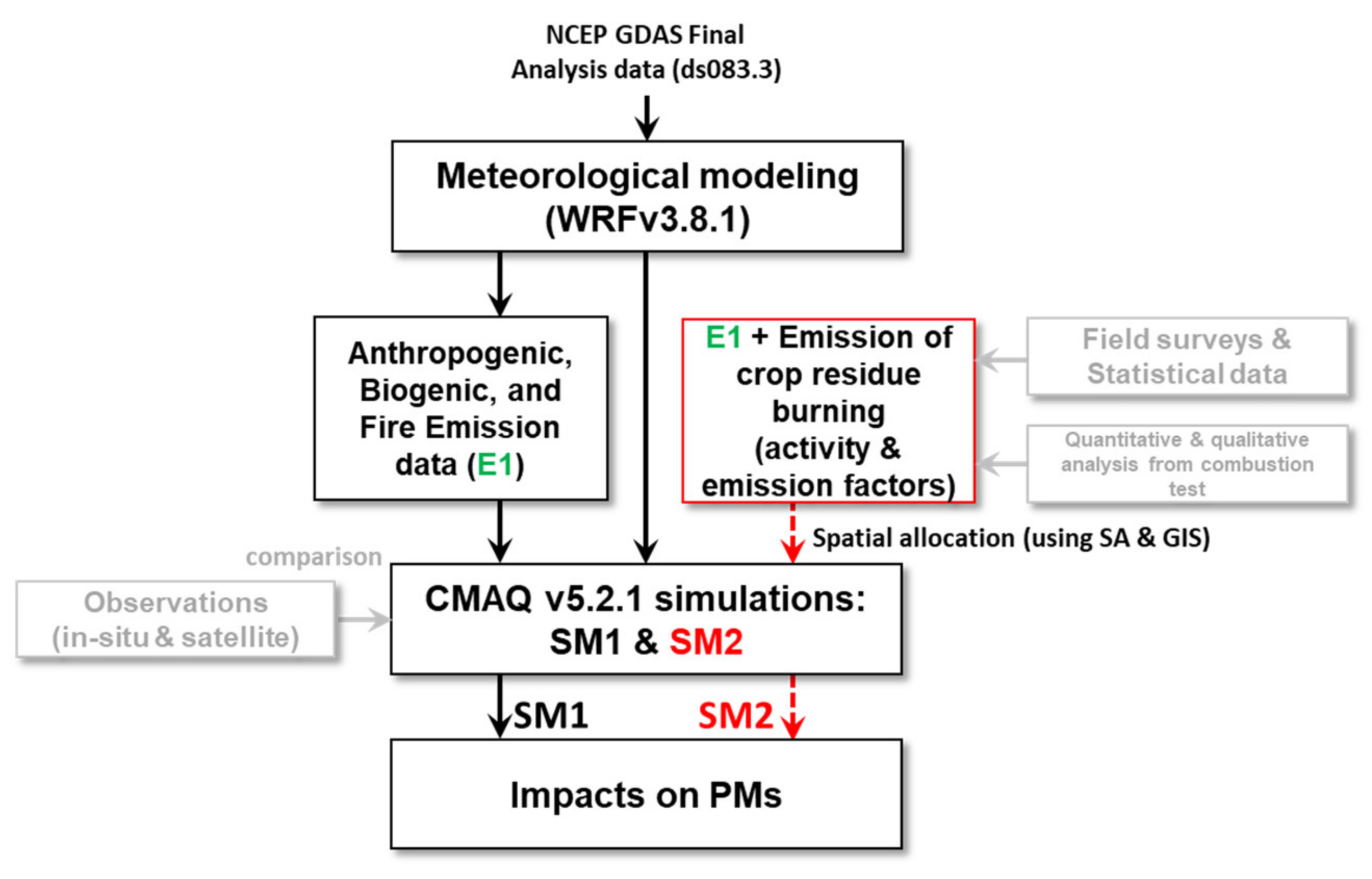
2.1. WRF-CMAQ Model Simulations

A 3-dimensional Eulerian Chemistry Transport Model (3D-CTM), US-EPA Models-3/CMAQ is one of the most powerful tools to manage the air quality for environmental policymakers and understand atmospheric phenomena for atmospheric scientists. The CMAQ model has been used worldwide to simulate the atmospheric levels of multi-pollutants, particularly focusing ozone and particulate matter, on local and regional scales because it is well built up and parameterized in gas-phase/heterogeneous chemistry and aerosol dynamics/thermodynamics (refer to CMAQ user’s guide for more details [62,63]). In this study, we also utilized the CMAQ v5.2.1 model to simulate the air quality and examine the impact of crop residue burning (CRB) on the levels of particulate matter in South Korea during the year of 2016 [63]. The spatial domain of the simulations consists of 273 rows and 204 columns of 15 × 15 km2 resolution with 27 vertical layers from the surface to ~50 hPa over East Asia. The CMAQ model simulations were configured with Stateside Air Pollution Research Center-07 (SAPRC-07) for the gas-phase chemistry [64,65] and sixth-generation model CMAQ aerosol model (AERO6) for the aerosol dynamics [66,67]. For the horizontal advection in the CMAQ simulations, we utilized Yamartino (YAMO) scheme [68], showing good performance in terms of mass conservation [69,70]. Additionally, the Multiscale and ACM2 schemes were used for the horizontal and vertical mixing processes [71,72,73].
The CMAQ model was derived by the meteorological fields produced from the WRFv3.8.1 with the ARW dynamic solver [74]. The initial and boundary data were the National Center for Environmental Prediction (NCEP) Final operation global analysis (ds083.3) obtained from the NCAR (https://rda.ucar.edu accessed on 14 February 2022). These input data have a spatial resolution of 0.25° × 0.25° with a 6 h interval. The WRF simulations employed the single-moment 6-class for microphysics scheme [75]. Other physical methods were Yonsei University (YSU) PBL parameterization [76], Rapid Radiative Transfer Model (RRTM) scheme for long- and short-wave radiations [77], and Kain-Fritch scheme for cumulus physics [78]. The chemical and physical parameterizations are given in Table 2.

2.2. Emission Inventory
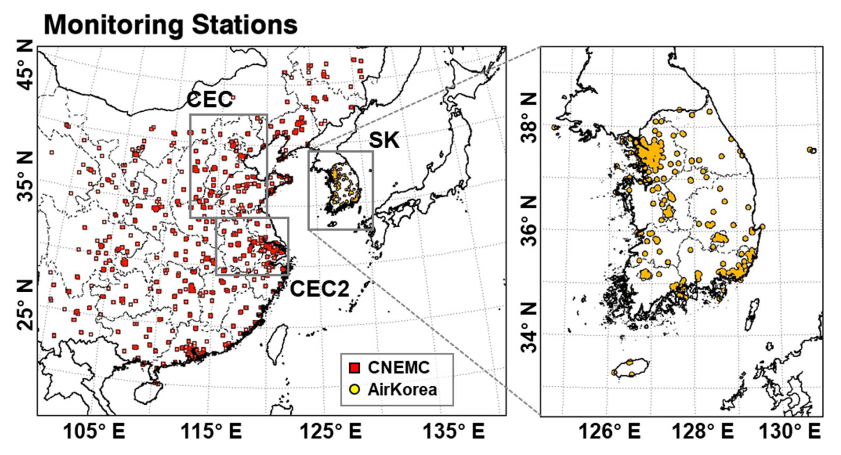
Atmospheric levels of gaseous and particulate species are significantly influenced by emission data [83]. For anthropogenic emission, we utilized the 0.1° × 0.1° resolved KORUS v5.0 emission inventory prepared from the SMOKE-Asia processing [84] over the entire domain except for South Korea. The emissions fluxes of CO, NOx, SO2, NH3, PM2.5, PM10, and total VOCs from the KORUS v5.0 were replaced with those from the 1 km × 1 km resolved Clean Air Policy Support System (CAPSS) inventory for South Korea. However, the KORUS v5.0 inventory was also used for information on the VOC speciation because the CAPSS inventory provided only total VOC emission fluxes instead of the speciated VOCs. For biogenic emissions, the Model of Emissions of Gases and Aerosol from Nature—Monitoring Atmospheric Composition and Climate (MEGAN-MACC) [85] was obtained from the monthly Emission of atmospheric Compounds and Compilation of Ancillary Data (ECCAD, https://eccad.aeris-data.fr/ accessed on 14 February 2022). For the fire emission, we also took into account the daily Fire Inventory from NCAR (FINN) v1.5 (https://www.acom.ucar.eud/Data/fire/ accessed on 14 February 2022) [55]. These emission data were spatially re-gridded into the model grids for the SM1 (default) simulation. The spatial distributions of emission fluxes used in the SM1 simulation were shown over South Korea and East Asia in Figure 3 and Figure S1, respectively.
In this study, monthly emissions of CO, NOx, SO2, NH3, PM2.5, PM10, and speciated VOCs from open burning of crop residue were estimated over South Korea using several activity data and emission factors. The monthly emissions (Eij) of pollutants (i) from residue burning of nineteen crops (j) were quantified from Equation (1) based on the methodology suggested by the studies of Delmas et al. [86], California Air Resources Board, US [87], and NSW Environment Protection Authority, Australia [88]. For the estimation, we considered nineteen crops, including rice (in the rice fields and ridges), barley, sweet potato, corn, soybean, pepper, sesame, perilla, peanut, garlic, onion, watermelon, apple, persimmon, citrus, pear, grape, and peach.
E i , j = j M j × E F i , j = j P j × R j × D j × F j × E F i , j
where, Mj represents masses of the residue of crop type j burned in the open field (unit: kg month−1) and is defined as the multiplication of Pj (production of crops, kg month−1), Rj (conversion factor for crop residue production or residue-to-crop ratio), Dj (correction factor for dry matter from the crop residues), and Fj (fraction of crop residue burning in the field). The production of crops (Pj) was obtained from Statistics Korea [89]. The conversion factors (Rj) were obtained from a report of the National Institute of Agricultural Sciences (NAS) in Korea [90] and summarized in Table S1. For other activity data, we carried out surveys (e.g., face-to-face, mail, and internet surveys) on the open burning of crop residue, targeting approximately 1000 farmers. The interviewees were selected considering their distributions of the agricultural areas and farmworkers by region. The questionnaire for the survey includes (i) what fraction of each crop residue is burned in the open field, (ii) how frequently, and (iii) which season the burning occurs in. In the study, to estimate the emission factors (EFi,j) of chemical species for 10 crops of rice, garlic, onion, sweet potato, barley, corn, peanut, watermelon, persimmon, and citrus fruit, the combustion test facility was built for the open combustion of crop residues under well-controlled conditions, which was designed based on the EPA method 5G [91]. The facility is composed of five components: (i) combustion chamber in which the crop residue is burned, (ii) inlet and outlet pipes, (iii) filter-based sampling part for PM10, PM2.5, EC, OC, and ion species, (iv) measuring part for VOCs, and (v) measuring part for other gases (e.g., NOx, CO, SO2, NH3). The schematic diagram for the combustion test facility is given in Figure S2. Then, particulate matters (PM10 and PM2.5) and gaseous species are analyzed qualitatively and quantitatively based on several analysis methods in Table S2. The emission factors of gaseous and particulate species were summarized in Table S3. The emission fluxes from the crop residue burning were estimated based on the municipal-level divisions (e.g., Si for the city, Gun for the county, and Gu for the district) in Korea. Finally, the emission fluxes based on the Si-Gun-Gu levels were spatially allocated to the modeling grids using the software of the Geographic Information System (GIS) and Spatial Allocator (SA). The spatial distributions of emission fluxes from the crop residue burning (CRB) were presented in the right two columns of Figure 3. The CRB emissions were then added into the default emission for the SM2 simulation.

2.3. Observations

The performance of the chemical model was evaluated by comparing the concentrations of O3, PM10, and PM2.5 observed at ~1400 sites in China and 320 sites in South Korea. These data were collected for the entire year of 2016 from both the China National Environmental Monitoring Center (CNEMC, https://quotsoft.net/air/ accessed on 14 February 2022) [92] in China and the national air quality monitoring network (AirKorea, https://www.airkorea.or.kr/ accessed on 14 February 2022) [93] in South Korea (Figure 4).
In addition to the ground data, satellite-observed data were also collected from TEMIS (www.temis.nl accessed on 14 February 2022) [94] for evaluation over the entire domain. The Ozone Monitoring Instrument (OMI) observation data retrieved from the Quality Assurance for Essential Climate Variables (QA4ECV) algorithm provides the tropospheric vertical NO2 columns on a daily basis. We extracted and utilized only valid data according to several flag criteria (e.g., processing_error_flag = 0; solar_zenith_angle < 80; snow_ice_flag < 10 or snow_ice_flag = 255; amf_trop/amf_geo > 0.2; cloud_radiance_fraction_no2 < 0.5) suggested in the document for the QA4ECV product [95]. Averaging kernels were also considered in the CMAQ-simulated NO2 columns for direct comparison with the OMI observations [96].

3. Results and Discussion

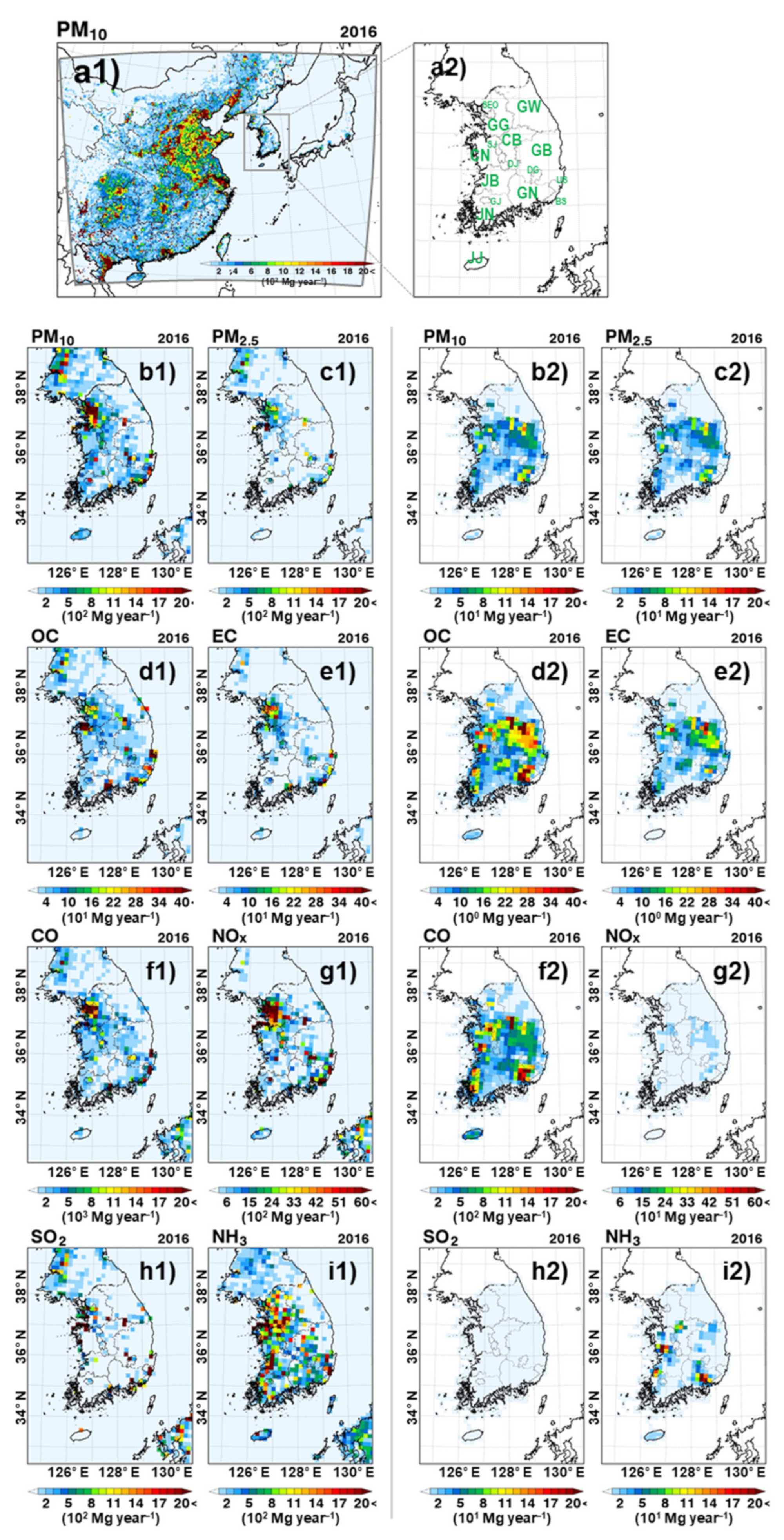
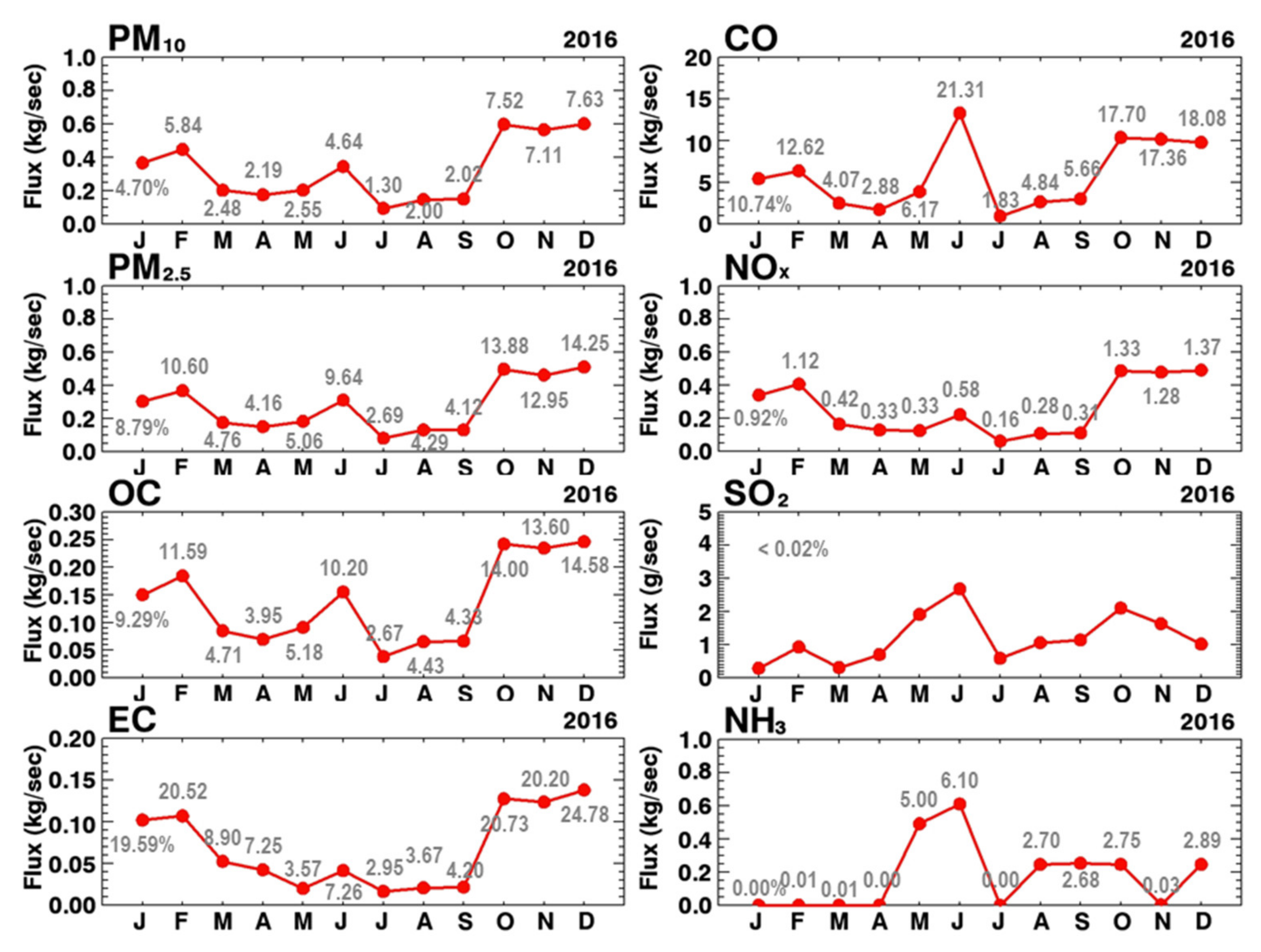
3.1. Emission Fluxes (E) Estimated from Residue Burning of Crops over South Korea

As discussed previously in Section 2.2, the CRB emission fluxes (Ei,j) were estimated from several emission factors (EFi,j) and activity data (Mj) related to crop residue burning. The annual emission fluxes over South Korea estimated as 9514, 8089, 4002, 2010, 172,407, 7675, 33, and 5053 Mg for PM10, PM2.5, OC, EC, CO, NOx (as NO2), SO2, and NH3, respectively (in Table 3), which corresponded to 4.16, 7.93, 8.21, 11.96, 10.27, 0.47, 0.01, and 1.86% of those from anthropogenic sources. The contributions from the crop residue burning to total emissions were not small, particularly for EC and CO, above 10%. However, such contributions can vary considerably depending on the analysis regions defined in Figure 3(a2). From a regional perspective, most species showed the highest emission fluxes in the order of Gyeongbuk (GB), Gyeongnam (GN), Chungbuk (CB), Chungnam (CN), and other provinces in Table 3. The high emissions were also clearly seen in the spatial distributions of CRB emission in Figure 3. GB province, the largest emitter of CRB, accounted for 33–41% and 14–37% for particulate and gaseous species, respectively. On the other hand, the CRB emissions in SEO, BS, DG, IC, GJ, DJ, US, and SJ were insignificant due to the limited cultivation areas in the metropolitan cities [89]. This shows a clear spatial contrast between the CRB and anthropogenic emissions (refer to Figure 3).
To evaluate the approximate magnitudes of emission fluxes in this study, we compared our estimations with data of Kim et al. (hereinafter referred to as KIM) [97], conducted for South Korea based on a similar bottom-up approach. Figure 5 showed scatter plots between KIM and our estimates for available species of PM2.5, PM10, CO, NOx, SO2, and NH3. In this analysis, emission fluxes in CN province also included those of SJ province. As shown in Figure 5, many data points were significantly scattered along the 1:1 line. Those were possibly due to two aspects. For the first, we considered seven more crops of persimmon, citrus fruit, sweet potato, rice, garlic, watermelon, and onion than those in KIM, leading to data points distributed above the 1:1 line (i.e., higher estimates). Secondly, the emission factors (EF) for barley were significantly different. The EFPM2.5, EFPM10, and EFCO of KIM were 6–15 times larger than our experiment values. In contrast to the first aspect, data points can be distributed below the 1:1 line. In the scatter plot for NH3, the large biases were determined dominantly by the high EFNH3 for watermelon, considered only in our estimate (Table S3). Nevertheless, both estimates were not significantly different in their magnitudes. Additionally, in both studies, GB province was ranked the highest in common for PM2.5, PM10, CO, and NOx. Annual emission fluxes from our estimate and KIM were summarized in Table S4.
Figure 6 shows monthly variations of CRB emissions of gaseous and particulate species over South Korea. As shown in Figure 6, while the CRB emission fluxes were generally high in the warm season, particularly in June for the gaseous species of CO, SO2, and NH3, they were great in the cold season for the particulate species of PMs, EC, and OC. Such differences are significantly related to the harvest time for the specific crop with its different emission factors for the chemical species. Accordingly, different harvest times and emission factors for the crops also led to significant differences in the monthly contributions. For example, the contributions were generally marginal within 0.02, 1.37, and 6.10% for the gaseous species of SO2, NOx, and NH3 (in the right column of Figure 6), respectively. On the other hand, the maximum contributions reached 14.25, 14.58, and 24.78% for PM2.5, OC, and EC (in the left columns of Figure 6), respectively. The emission fluxes of EC were relatively small compared to those of PM10 and PM2.5, despite it being the highest contribution.
For anthropogenic and CRB sources, we also examined the ratio of PM2.5 to PM10 emissions in this study. The ratios can be used to identify the sources because the particulate matter in different sizes possibly originates from different sources [98,99]. In the anthropogenic emissions from the CAPSS inventory, the monthly PM2.5/PM10 ratios were almost constant, ranging between 0.41 and 0.44. For the CRB emission, the average ratio was 0.85 in the range of 0.82–0.90, indicating relatively large amounts of PM2.5 emitted through the agricultural residue burning. Our averaging ratios for the CRB emission are similar to values from observations during the periods of biomass burning events at Gwangju Korea and Pathumthani Thailand [100,101].

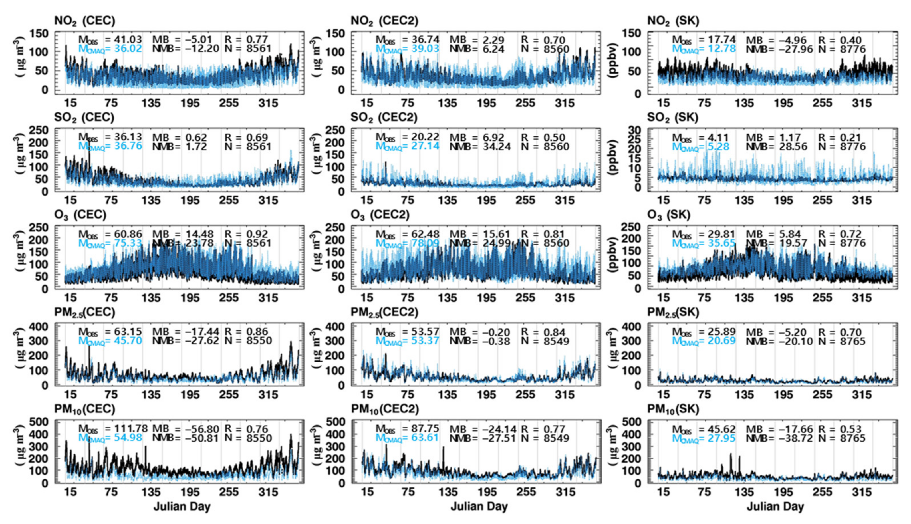
3.2. Modeling Performances

We evaluated the general performances of the default CMAQ simulation (i.e., SM1) by comparing the tropospheric NO2 columns over the entire domain. The hourly mixing ratios (unit: ppm) of NO2 at each layer from the simulations were converted to the vertical column concentrations (unit: molecules cm−2) by integrating vertically from surface to approximately 10 km in altitude for direct comparison [102].
The first and second columns of Figure 7 showed spatial and seasonal distributions of the CMAQ-calculated and OMI-retrieved NO2 columns over East Asia. The differences and scatter plots between the two columns were presented in the third and fourth columns of Figure 7. The simulated NO2 columns over the entire domain were 0.85 × 10¹⁵, 0.52 × 10¹⁵, 1.12 × 10¹⁵, 1.89 × 10¹⁵ molecules cm−2 for spring (March–May), summer (June–August), fall (September–November), and winter (December–February), respectively. These values were small, compared to those of OMI observation, which were 2.15 × 10¹⁵, 1.61 × 10¹⁵, 2.15 × 10¹⁵, 2.87 × 10¹⁵ molecules cm−2 for spring, summer, fall, and winter, respectively. Despite some positive bias (showing red) partly over Hebei and Henan provinces, such negative bias (showing blue color) was seen over most regions, particularly in central east China and the Guangdong and Hong Kong areas in the third column of Figure 7 (also refer to the statistical values and slopes in the fourth column of the figure), indicating the underestimation of NOx emissions in these areas. According to the study of ozone production efficiency (OPE) by Oak et al. [103] using KORUSv5 emission data, the OPE characteristics are best simulated when 50% of NOx emission increase in the chemistry-transport modeling. Such results also indicate the underestimation of KORUSv5 NOx emissions used in our study. Nevertheless, our CMAQ simulations using the same emission inventory well captured the satellite-observed spatial distributions and seasonal variations over East Asia. The correlation coefficients were quite good, ranging between 0.85 and 0.88. During the summer episode, the lower concentration observed from the OMI sensor was also well simulated by the CMAQ model in the second row of Figure 7. The low NO2 columns in summer are attributed to the active NOx chemical losses via the reaction of NO2 with high concentrations of OH radicals [104,105].
In addition to satellite, in situ ground observations from the CNEMN and AirKorea were utilized to evaluate the modeling performance. The hourly observation was compared to the simulated data averaged for the pixels corresponding to the CEC, CEC2, and SK regions defined in Figure 4. Figure 8 showed the time series of hourly surface concentrations of O3, PM10, and PM2.5 from observations (black lines) and simulations (blue lines) for CEC, CEC2, and SK in the first, second, and third columns, respectively.
In the upper panel of Figure 8, the simulated O3 concentrations were higher by 20–25%, compared to the observation. The high O3 mixing ratios simulated from the CMAQ simulation are strongly related to the underestimation of NOx emissions over East Asia discussed in the NO2 column analysis in Figure 7 because of less O3 being titrated by NO. The correlation coefficients were good, generally ranging from 0.72 to 0.91. In Figure S3, the model-calculated O3 mixing ratios agreed spatially with monthly averaged values of in situ observation, particularly in Seoul Metropolitan areas (showing bluish colors in the figure).
In the bottom panel of Figure 8, the simulated concentrations of PM10 were small by −50.8, −25.5, and −38.7%, compared to the observations over CEC, CEC2, and SK. Nevertheless, the correlation coefficients between the simulated and observed PM10 were moderately good (0.76 and 0.77) over CEC and CEC2. The observations captured the Asian dust in China and its impact on PM10 in South Korea in May and June 2016. However, the high concentrations of PM10 were not adequately simulated in the CMAQ simulations, in which the dust module for dust emission was off. The lower correlation coefficient in SK was mainly due to some inconsistency, particularly during April–June (refer to Figure S4). It is well known that the concentration of PM10 is closely related to the Asian dust event [106].
On the other hand, the temporal variations and magnitudes of observed PM2.5 were well simulated, as shown in the middle panel of Figure 8. Accordingly, the correlation coefficients for PM2.5 were good as 0.87, 0.84, and 0.70 over CEC, CEC2, and SK, respectively. Although the simulated PM2.5 concentrations were also small by −27.6, −0.4, and −20.1% over the analysis regions, PM2.5 was better simulated than PM10 in terms of several statistical parameters between simulations and observations (i.e., absolute and relative differences, correlation coefficient, and slope in the scatter plots). Additionally, the spatial distributions of PM2.5 concentrations were well consistent with those of in situ observation in Figure S5. Therefore, we more focused on PM2.5 for the impacts of crop residue burning.
Collectively, the performance for SM1 simulation showed underestimation of PM10 and O3 in the CEC region, which affects the air quality in South Korea. Nevertheless, there were relatively consistent for PM2.5. From the statistical analysis between the simulated and observed O3 and PM2.5 concentrations, we believe that the SM1 simulation has sufficient performance to investigate the effect of the CRB emission on particulate matter in South Korea.

3.3. Impact of Crop Residue Burning on Particulate Matters

The impact of the crop residue burning on the concentrations of particulate matter was examined in terms of absolute (unit: μg m−3) and relative (unit: %) differences using Equations (2) and (3) as follows:
A .   D i f f = C S M 2 C S M 1
R .   D i f f = C S M 2 C S M 1 C S M 1 × 100
where, CSM1 and CSM2 represent the concentrations of PM2.5 or PM10 from the SM1 and SM2 simulations, respectively. Figure 9 and Figure 10 show the spatial distributions of absolute and relative differences of PM2.5 between the SM1 and SM2 simulations over South Korea. The positive values of the absolute differences colored in red in Figure 9 indicate the elevated PM2.5 originated from the crop residue burning. The absolute differences were lowest at 0.07 μg m−3 in July and were generally high in June, October, November, and December (highest at 0.55 μg m−3 in October). The monthly absolute difference increased to a maximum of 1.82 μg m−3 at a specific pixel of GN province (defined in Figure 9) in June.
The relative difference at the same specific pixel point in GN province also increased by 12.91% in June. From a temporal viewpoint, the relative differences were highest (4.33%) in October and lowest (0.60%) in March. From a spatial point of view, the relatively high elevations occurred in the rural areas of the northern GB, central GN, northern CB, southern CN areas. For PM10 in this study, we also examined the absolute and relative differences in Figures S6 and S7. As shown in the analysis, the temporal and spatial features for PM10 were not much different from those for PM2.5.
From such analysis, most increases in the PM10 concentration were attributed to the increase in the PM2.5 concentration. The result was consistent with the PM2.5/PM10 emission ratios discussed in Section 3.1. Because PM2.5 has a more severe impact on cardiorespiratory disorders than PM10, the high ratios are more important from a public health perspective [107].
We summarized the impacts of CRB on the monthly mean and maximum concentrations of surface PM2.5 and PM10 in terms of absolute (AD) and relative differences (RD) in Table 4 and Table 5. Collectively, our simulations showed that over the entire period of 2016 in South Korea, the monthly PM2.5 (and PM10) concentrations originated by the crop residue burning were elevated within 0.55 μg m−3 (and 0.60 μg m−3).
The contributions from the CRB emissions to the concentrations of particulate matter estimated in this study are still subject to some uncertain issues. The uncertainty is related to the diurnal variations of the CRB emissions. Although the contributions in this study were estimated every month, the diurnal variations of CRB emissions can be randomly large. Open crop residue burning activity has often been carried out surreptitiously in the dark evening in South Korea to avoid surveillance for the illegal burning [50,108]. Thus, the peak contribution occurs possibly between late evening and early night during the day. As the planetary boundary layer (PBL) decreases at that temporal point, the surface concentrations of particulate matter or its contribution can further increase [109]. However, the time of open burning during the day varies spatially, depending on country-specific agricultural practices [44,50]. Additionally, as input data for the estimation, the activity data still has room for improvement through the precise representativeness of the survey population to the reality.

4. Summary and Conclusions

In this study, we attempted to quantify the impacts of crop residue burning (CRB) on the concentrations of PM10 and PM2.5 in South Korea. For the investigation, we built the CRB emission database on the basis of the bottom-up approach over South Korea. Then, two different one-year WRF-CMAQ simulations with and without the CRB emissions were conducted for 2016.
The monthly CRB emissions over South Korea were estimated using i) several activity data of nineteen crops from the online and offline surveys with statistical data in Korea and ii) emission factors for the gaseous and particulate species through a combustion test facility. In our estimation, the emissions of CRB over South Korea are 9514, 8089, 4002, 2010, 172,407, 7675, 33, and 5053 Mg year−1 for PM10, PM2.5, OC, EC, CO, NOx (as NO2), SO2, and NH3, respectively. The contributions of the CRB emissions to the anthropogenic emissions were generally small, except for EC and OC, which have more than 10% contributions. In the regional comparison with the KIM study [97] over South Korea, our estimates were not significantly different except for NH3 and SO2 species. In both studies, Gyeongbuk (GB) province was the largest emitter of CRB emission in common for PM2.5, PM10, CO, and NOx. The CRB emissions in GB accounted for approximately 33–41% of the total amounts for the particulate species. In terms of seasonal variation, the crop residue burning emissions were high in the cold season for PM10, PM2.5, EC, and OC. On the other hand, they were higher in the warm season for CO, SO2, and NH3.
From two different WRF-CMAQ simulations, we found the monthly average concentrations of PM2.5 (PM10) over South Korea were elevated between 0.07 and 0.55 μg m−3 (between 0.07 and 0.60 μg m−3) when the CRB missions are considered in the CMAQ simulation. The elevations in PM2.5 (PM10) were corresponded to 0.6–4.3% (0.5–3.1%) in relative differences. The increases in PM2.5 were high in June, October, November, and December. Spatially, the relatively high elevations occurred in the northern Gyeongbuk (GB), central Gyeongnam (GN), northern Chungbuk (CB), and southern Chungnam (CN) provinces in South Korea.
Despite large uncertainties in the activity data, our crop residue burning emission from this study is expected to be an alternative database for the areas where the satellite observations for the top-down estimation are not available, in part, for small and short-lasting fires or cloudy conditions. The emission data can also be applied to the air quality modeling to evaluate the associated disease/public health burden and impact on climate change. Finally, our analysis contributes to determining the effectiveness of the reduction measure when the Korean government establishes the reduction policy to reduce the concentrations of PM10 and PM2.5. From the study, the impact of the CRB emissions on PM10 and PM2.5 were marginal over South Korea. Nevertheless, the impacts could vary significantly from a temporal and spatial point of view. Thus, further studies should investigate the in-depth diurnal/temporal variations of the crop residue burning emissions based on the combined top-down and bottom-up approaches.

Supplementary Materials

The following supporting information can be downloaded at: https://www.mdpi.com/article/10.3390/atmos13040559/s1, Figure S1: Annual emission fluxes of (a) PM10, (b) PM2.5, (c) OC, (d) EC, (e) CO, (f) NO, (g) SO2, and (h) NH3 combined from the KORUS v5, MEGAN, and FINN v1.5 inventories used in the SM1 simulation; Figure S2: Schematic diagram of combustion test facility; Figure S3: Spatial distributions of O3 mixing ratios from the SM1 simulations over South Korea. The colored circles represented the observed values from the AirKorea network (unit: ppb); Figure S4: Spatial distributions of PM10 concentrations from the SM1 simulations over South Korea. The colored circles represented the observed values from the AirKorea network (unit: μg m−3); Figure S5: Spatial distributions of PM2.5 concentrations from the SM1 simulations over South Korea. The colored circles represented the observed values from the AirKorea network (unit: μg m−3); Figure S6: Absolute differences for PM10; Figure S7: Relative differences for PM10; Table S1: Residue-to-crop ratios for crops considered in this study; Table S2: Analytic methods for gaseous and particulate species; Table S3: Examples of emission factors (Ei,j) of particulate and gaseous species for the crop residue (Unit: g/kg); Table S4: Estimated CRB emission and their comparison with Kim et al. [97] (unit: g/kg). Additional information are explained in [110,111] in the Supplementary Material file.

Author Contributions

Conceptualization, K.M.H. and B.T.L.; methodology, K.M.H., B.T.L., and M.-S.B.; validation, K.M.H., S.L., C.H.J., and H.S.K.; formal analysis, B.T.L., M.-S.B., C.H.J., and K.M.H.; data curation, S.L.; writing—review and editing, K.M.H., S.L., C.H.J., and B.T.L. All authors have read and agreed to the published version of the manuscript.

Funding

This work was supported by the Korea Institute of Planning and Evaluation for Technology in Food, Agriculture and Forestry (IPET) through the Agri-Bio industry Technology Development Program, funded by the Ministry of Agriculture, Food and Rural Affairs (MAFRA) (319108-2). Additionally, this research was funded by a National Research Foundation of Korea Grant from the Korean Government (MSIT; the Ministry of Science ICT) (NRF-2021M1A5A1065425) (KOPRI-PN21011). C.H. Jung was supported by the National Research Foundation of Korea grant funded by the Korean government (MSIT) (No. NRF-2021R1F1A1046878).

Institutional Review Board Statement

Not applicable.

Informed Consent Statement

Not applicable.

Data Availability Statement

Not applicable.

Acknowledgments

We would like to acknowledge the use of the emission data from the websites (https://eccad.aeris-data.fr/ accessed on 14 February 2022; https://www.acom.ucar.edu/Data/fire/ accessed on 14 February 2022). We also thank the OMI data team for developing the NO2 product (https://www.temis.nl/airpollution/no2col/no2regioomi_qa.php accessed on 14 February 2022). Additionally, we are thankful to all scientists and operators for the uses of in situ ground data in China and South Korea.

Conflicts of Interest

The authors declare no conflict of interest.

References

  1. Kim, Y.P.; Lee, G.W. Trend of air quality in Seoul: Policy and Science. Aerosol Air Qual. Res. 2018, 18, 2141–2156. [Google Scholar] [CrossRef] [Green Version]
  2. Koo, J.H.; Kim, J.; Lee, Y.G.; Park, S.S.; Lee, S.; Chong, H.; Cho, Y.; Kim, J.; Choi, K.; Lee, T. The implication of the air quality pattern in South Korea after the COVID-19 outbreak. Sci. Rep. 2020, 10, 22462. [Google Scholar] [CrossRef] [PubMed]
  3. Ministry of Environment in South Korea. Available online: http://eng.me.go.kr/eng/web/index.do?menuId=464 (accessed on 21 January 2022).
  4. World Health Organization. WHO Global Air Quality Guidelines: Particulate Matter (PM2.5 and PM10), Ozone, Nitrogen Dioxide, Sulfur Dioxide, and Carbon Monoxide. Available online: https://apps.who.int/iris/handle/10665/345329 (accessed on 21 January 2022).
  5. Yevich, R.; Logan, J.A. An assessment of biofuel use and burning of agricultural waste in the developing world. Glob. Biogeochem. Cycles 2003, 17, 1095. [Google Scholar] [CrossRef]
  6. Wulfhorst, J.D.; Van Tassell, L.; Johnson, B.; Holman, J.; Thill, D. An Industry Amidst Conflict and Change: Practices and Perceptions of Idaho’s Bluegrass Seed Producers; University of Idaho College of Agricultural and Life Sciences: Moscow, ID, USA, 2006; pp. 1–20. [Google Scholar]
  7. Lin, N.-H.; Tsay, S.-C.; Maring, H.B.; Yen, M.-C.; Sheu, G.-R.; Wang, S.-H.; Chi, K.H.; Chuang, M.-T.; Ou-Yang, C.-F.; Fu, J.-S.; et al. An overview of regional experiments on biomass burning aerosols and related pollutants in Southeast Asia: From BASE-ASIA and the Dongsha Experiment to 7-SEAS. Atmos. Environ. 2013, 78, 1–19. [Google Scholar] [CrossRef] [Green Version]
  8. Zhou, L.; Baker, K.R.; Napelenok, S.L.; Pouliot, G.; Elleman, R.; O’Neill, S.M.; Urbanski, S.P.; Wong, D.C. Modeling crop residue burning experiments to evaluate smoke emissions and plume transport. Sci. Total Environ. 2018, 627, 523–533. [Google Scholar] [CrossRef] [PubMed]
  9. Jethva, H.; Torres, O.; Field, R.D.; Lyapustin, A.; Gautam, R.; Kayetha, V. Connecting crop productivity, residue fires, and air quality over Northern India. Sci. Rep. 2019, 9, 16594. [Google Scholar] [CrossRef] [PubMed] [Green Version]
  10. Takami, K.; Shimadera, H.; Uranishi, K.; Kondo, A. Impacts of Biomass Burning Emission Inventories and Atmospheric Reanalyses on Simulated PM10 over Indochina. Atmosphere 2020, 11, 160. [Google Scholar] [CrossRef] [Green Version]
  11. Das, B.; Bhave, P.V.; Puppala, S.P.; Shakya, K.; Maharjan, B.; Byanju, R.M. A model-ready emission inventory for crop residue open burning in the context of Nepal. Environ. Pollut. 2020, 266, 115069. [Google Scholar] [CrossRef] [PubMed]
  12. Crutzen, P.J.; Andreae, M.O. Biomass burning in the tropics: Impact on atmospheric chemistry and biogeochemical cycles. Science 1990, 250, 1669–1678. [Google Scholar] [CrossRef] [PubMed]
  13. Reisen, F.; Meyer, C.P.; Keywood, M.D. Impact of biomass burning sources on seasonal aerosol air quality. Atmos. Environ. 2013, 67, 437–447. [Google Scholar] [CrossRef]
  14. Agarwal, R.; Awasthi, A.; Mital, S.K.; Singh, N.; Gupta, P.K. Statistical model to study the effect of agriculture crop residue burning on healthy subjects. MAPAN-J. Metrol. Soc. India 2014, 29, 57–65. [Google Scholar] [CrossRef]
  15. Awasthi, A.; Agarwal, R.; Mittal, S.K.; Singh, N.; Singh, K.; Gupta, P.K. Study of size and mass distribution of particulate matter due to crop residue burning with seasonal variation in rural area of Punjab, India. J. Environ. Monit. 2011, 13, 1073–1081. [Google Scholar] [CrossRef] [PubMed] [Green Version]
  16. Chen, Y.; Xie, S. Characteristics and formation mechanism of a heavy air pollution episode caused by biomass burning in Chengdu, Southwest China. Sci. Total Environ. 2014, 473–474, 507–517. [Google Scholar] [CrossRef] [PubMed]
  17. Yang, S.; He, H.; Lu, S.; Chen, D.; Zhu, J. Quantification of crop residue burning in the field and its influence on ambient air quality in Suqian, China. Atmos. Environ. 2008, 42, 1961–1969. [Google Scholar] [CrossRef]
  18. Zhang, H.; Ye, X.; Cheng, T.; Chen, J.; Yang, X. A laboratory study of agricultural crop residue combustion in China: Emission factors and emission inventory. Atmos. Environ. 2008, 42, 8432–8441. [Google Scholar] [CrossRef]
  19. Jain, N.; Bhatia, A.; Pathak, H. Emission of air pollutants from crop residue burning in India. Aerosol Air Qual. Res. 2014, 14, 422–430. [Google Scholar] [CrossRef] [Green Version]
  20. Andreae, M.O.; Merlet, P. Emission of trace gases and aerosols from biomass burning. Glob. Biogeochem. Cycles 2001, 15, 955–966. [Google Scholar] [CrossRef] [Green Version]
  21. Stockwell, C.E.; Christian, T.J.; Goetz, J.D.; Jayarathne, T.; Bhave, P.V.; Praveen, P.S.; Adhikari, S.; Maharjan, R.; DeCarlo, P.F.; Stone, E.A.; et al. Nepal Ambient Monitoring and Source Testing Experiment (NAMaSTE): Emissions of trace gases and lightabsorbing carbon from wood and dung cooking fires, garbage and crop residue burning, brick kilns, and other sources. Atmos. Chem. Phys. 2016, 16, 11043–11081. [Google Scholar] [CrossRef] [Green Version]
  22. Jayarathne, T.; Stockwell, C.E.; Bhave, P.V.; Praveen, P.S.; Rathnayake, C.M.; Islam, M.R.; Panday, A.K.; Adhikari, S.; Maharjan, R.; Goetz, J.D.; et al. Nepal Ambient Monitoring and Source Testing Experiment (NAMaSTE): Emissions of particulate matter from wood and dung cooking fires, garbage and crop residue burning, brick kilns, and other sources. Atmos. Chem. Phys. 2018, 18, 2259–2286. [Google Scholar] [CrossRef] [Green Version]
  23. McCarty, J.L. Remote Sensing-Based Estimates of Annual and Seasonal Emissions from Crop Residue Burning in the Contiguous United States. J. Air Waste Manag. Assoc. 2011, 61, 22–34. [Google Scholar] [CrossRef]
  24. Turn, S.Q.; Jenkins, B.M.; Chow, J.C.; Pritchett, L.C.; Campbell, D.; Cahill, T.; Whalen, S.A. Elemental Characterization of Particulate Matter Emitted from Biomass Burning: Wind Tunnel Derived Source Profiles for Herbaceous and Wood Fuels. J. Geophys. Res. 1997, 102, 3683–3699. [Google Scholar] [CrossRef]
  25. Liu, M.; Song, Y.; Yao, H.; Kang, Y.; Li, M.; Huang, X.; Hu, M. Estimating emissions from agricultural fires in the North China Plain based on MODIS fire radiative power. Atmos. Environ. 2015, 112, 326–334. [Google Scholar] [CrossRef]
  26. Akagi, S.; Yokelson, R.J.; Wiedinmyer, C.; Alvarado, M.; Reid, J.; Karl, T.; Crounse, J.; Wennberg, P. Emission factors for open and domestic biomass burning for use in atmospheric models. Atmos. Chem. Phys. 2011, 11, 4039–4072. [Google Scholar] [CrossRef] [Green Version]
  27. Wooster, M.J.; Roberts, G.; Perry, G.; Kaufman, Y. Retrieval of biomass combustion rates and totals from fire radiative power observations: FRP derivation and calibration relationships between biomass consumption and fire radiative energy release. J. Geophys. Res. Atmos. 2005, 110, D24311. [Google Scholar] [CrossRef]
  28. Li, J.; Li, Y.; Bo, Y.; Xie, S. High-resolution historical emission inventories of crop residue burning in fields in China for the period 1990–2013. Atmos. Environ. 2016, 138, 152–161. [Google Scholar] [CrossRef]
  29. Li, X.G.; Wang, S.X.; Duan, L.; Hao, J.; Li, C.; Chen, Y.S.; Yang, L. Particulate and trace gas emissions from open burning of wheat straw and corn stover in China. Environ. Sci. Technol. 2007, 41, 6052–6058. [Google Scholar] [CrossRef]
  30. Zhang, Y.; Shao, M.; Lin, Y.; Luan, S.; Mao, N.; Chen, W.; Wang, M. Emission inventory of carbonaceous pollutants from biomass burning in the Pearl River Delta Region, China. Atmos. Environ. 2013, 76, 189–199. [Google Scholar] [CrossRef]
  31. National Bureau of Statistics of China, 1991–2014. China Statistical Yearbook; China Statistics Press: Beijing, China, 2014. [Google Scholar]
  32. Wang, X.Y.; Xue, S.; Xie, G.H. Value-taking for residue factor as a parameter to assess the field residue of field crops. J. China Agric. Univ. 2012, 17, 1–8. (In Chinese) [Google Scholar]
  33. Andela, N.; Van, D.W.; Guido, R.; Kaiser, J.W.; Van Leeuwen, T.T.; Wooster, M.J.; Lehmann, C.E.R. Biomass burning fuel consumption dynamics in the tropics and subtropics assessed from satellite. Biogeosciences 2016, 13, 3717–3734. [Google Scholar] [CrossRef] [Green Version]
  34. Pouliot, G.; Rao, V.; McCarty, J.L.; Soja, A. Development of the crop residue and rangeland burning in the 2014 National Emissions Inventory using information from multiple sources. J. Air Waste Manag. Assoc. 2017, 67, 613–622. [Google Scholar] [CrossRef] [Green Version]
  35. Van der Werf, G.R.; Randerson, J.T.; Giglio, L.; van Leeuwen, T.T.; Chen, Y.; Rogers, B.M.; Mu, M.; van Marle, M.J.E.; Morton, D.C.; Collatz, G.J.; et al. Global fire emissions estimates during 1997–2016. Earth Syst. Sci. Data 2017, 9, 697–720. [Google Scholar] [CrossRef] [Green Version]
  36. Giglio, L.; Randerson, J.T.; van der Werf, G.R. Analysis of daily, monthly, and annual burned area using the fourth generation global fire emissions database (GFED4). J. Geophys. Res.-Biogeo. 2013, 118, 317–328. [Google Scholar] [CrossRef] [Green Version]
  37. Randerson, J.T.; Chen, Y.; van der Werf, G.R.; Rogers, B.M.; Morton, D.C. Global burned area and biomass burning emissions from small fires. J. Geophys. Res.-Biogeo. 2012, 117, G04012. [Google Scholar] [CrossRef]
  38. Wu, J.; Kong, S.; Wu, F.; Cheng, Y.; Zheng, S.; Yan, Q.; Zheng, H.; Yang, G.; Zheng, M.; Liu, D. Estimating the open biomass burning emissions in central and eastern China from 2003 to 2015 based on satellite observation. Atmos. Chem. Phys. 2018, 18, 11623–11646. [Google Scholar] [CrossRef] [Green Version]
  39. He, M.; Wang, X.R.; Han, L.; Feng, X.Q.; Mao, X. Emission Inventory of Crop Residues Field Burning and Its Temporal and Spatial Distribution in Sichuan Province. Environ. Sci. 2015, 36, 1208–1216. (In Chinese) [Google Scholar]
  40. Yin, L.; Du, P.; Zhang, M.; Liu, M.; Xu, T.; Song, Y. Estimation of emissions from biomass burning in China (2003–2017) based on MODIS fire radiative energy data. Biogeosciences 2019, 16, 1629–1640. [Google Scholar] [CrossRef] [Green Version]
  41. Li, F.; Zhang, X.; Roy, D.P.; Kondragunta, S. Estimation of biomass-burning emissions by fusing the fire radiative power retrievals from polar-orbiting and geostationary satellite across the conterminous United States. Atmos. Environ. 2019, 211, 274–287. [Google Scholar] [CrossRef]
  42. Shi, Y.; Zang, S.; Matsunaga, T.; Yamaguchi, Y. A multi-year and high-resolution inventory of biomass burning emissions in tropical continents from 2001–2017 based on satellite observations. J. Clean. Prod. 2020, 270, 122511. [Google Scholar] [CrossRef]
  43. Liu, T.; Marlier, M.E.; Karambelas, A.; Jain, M.; Singh, S.; Singh, M.K.; Gautam, R.; DeFries, R.S. Missing emissions from post-monsoon agricultural fires in northwestern India: Regional limitations of MODIS burned area and active fire products. Environ. Res. Commun. 2019, 1, 011007. [Google Scholar] [CrossRef]
  44. Liu, T.; Mickley, L.J.; Singh, S.; Jain, M.; DeFries, R.S.; Marlier, M.E. Crop residue burning practices across north India inferred from household survey data: Bridging gaps in satellite observations. Atmos. Environ. X 2020, 8, 1000091. [Google Scholar] [CrossRef]
  45. Andela, N.; Morton, D.C.; Giglio, L.; Paugam, R.; Chen, Y.; Hantson, S.; van der Werf, G.R.; Randerson, J.T. The Global Fire Atlas of individual fire size, duration, speed, and direction. Earth Syst. Sci. Data 2019, 11, 529–552. [Google Scholar] [CrossRef] [Green Version]
  46. Lasko, K.; Vadrevu, K. Improved rice residue burning emissions estimates: Accounting for practice-specific emission factors in air pollution assessments of Vietnam. Environ. Pollut. 2018, 236, 795–806. [Google Scholar] [CrossRef] [PubMed]
  47. Kaiser, J.W.; Andela, N.; Atherton, J.; de Jong, M.; Heil, A.; Paugam, R.; Remy, S.; Schultz, M.G.; van der Werf, G.R.; van Leeuwen, T.T.; et al. Recommended Fire Emission Service Enhancements. ECMWF Technical Memoranda; ECMWF: Reading, UK, 2014. [Google Scholar]
  48. Bouwman, L.; Braatz, B.; Conneely, D.; Gaffney, K.; Gerbens, S.; Gibbs, M.; Hao, W.M.; Johnson, D.; Jun, P.; Lassey, K.; et al. Chapter 4: Agriculture. In IPCC Good Practice Guidance and Uncertainty Management in National Greenhouse Gas Inventories; IPCC-NGGIP: Kanagawa, Japan, 2000. [Google Scholar]
  49. Ravindranath, N.H.; Somashekar, H.I.; Nagaraja, M.S.; Sudha, P.; Sangeetha, G.; Bhattacharya, S.C.; Abdul Salam, P. Assessment of sustainable non-plantation biomass resources potential for energy in India. Biomass Bioenergy 2005, 29, 178–190. [Google Scholar] [CrossRef]
  50. Shen, Y.; Jiang, C.; Chan, K.L.; Hu, C.; Yao, L. Estimation of Field-Level NOx Emissions from Crop Residue Burning Using Remote Sensing Data: A Case Study in Hubei, China. Remote Sens. 2021, 13, 404. [Google Scholar] [CrossRef]
  51. Qiu, X.; Duan, L.; Chai, F.; Wang, S.; Yu, Q.; Wang, S. Deriving High-Resolution Emission Inventory of Open Biomass Burning in China based on Satellite Observations. Environ. Sci. Technol. 2016, 50, 11779–11786. [Google Scholar] [CrossRef] [PubMed]
  52. Ellicott, E.; Vermote, E.; Giglio, L.; Roberts, G. Estimating biomass consumed from fire using MODIS FRE. Geophys. Res. Lett. 2009, 36, L13401. [Google Scholar] [CrossRef] [Green Version]
  53. Seiler, W.; Crutzen, P. Estimates of the gross and net flux of carbon between the biosphere and the atmosphere from biomass burning. Clim. Change 1980, 2, 207–247. [Google Scholar] [CrossRef]
  54. Kaufman, Y.J.; Justice, C.O.; Flynn, L.P.; Kendall, J.D.; Prins, E.M.; Giglio, L.; Ward, D.E.; Menzel, W.P.; Setzer, A.W. Potential global fire monitoring from EOS-MODIS. J. Geophys. Res. 1998, 103, 32215–32238. [Google Scholar] [CrossRef]
  55. Wiedinmyer, C.; Akagi, S.K.; Yokelson, R.J.; Emmons, L.K.; Al-Saadi, J.A.; Orlando, J.J.; Soja, A.J. The Fire INventory from NCAR (FINN): A high resolution global model to estimate the emissions from open burning. Geosci. Model Dev. 2011, 4, 625–641. [Google Scholar] [CrossRef] [Green Version]
  56. Wiedinmyer, C.; Yokelson, R.; Gullett, B.K. Global Emissions of Trace Gases, Particulate Matter, and Hazardous Air Pollutants from Open Burning of Domestic Waste. Environ. Sci. Technol. 2014, 48, 9523–9530. [Google Scholar] [CrossRef]
  57. Van der Werf, G.R.; Randerson, J.T.; Giglio, L.; Collatz, G.J.; Mu, M.; Kasibhatla, P.S.; Morton, D.C.; DeFries, R.S.; Jin, Y.; van Leeuwen, T.T. Global fire emissions and the contribution of deforestation, savanna, forest, agricultural, and peat fires (1997–2009). Atmos. Chem. Phys. 2010, 10, 11707–11735. [Google Scholar] [CrossRef] [Green Version]
  58. Kaiser, J.W.; Heil, A.; Andreae, M.O.; Benedetti, A.; Chubarova, N.; Jones, L.; Morcrette, J.J.; Razinger, M.; Schultz, M.G.; Suttie, M.; et al. Biomass burning emissions estimated with a global fire assimilation system based on observed fire radiative power. Biogeosciences 2012, 9, 527–554. [Google Scholar] [CrossRef] [Green Version]
  59. Xu, W.; Wooster, M.J.; Kaneko, T.; He, J.; Zhang, T.; Fisher, D. Major advances in geostationary fire radiative power (FRP) retrieval over Asia and Australia stemming from use of Himarawi-8 AHI. Remote Sens. Environ. 2017, 193, 138–149. [Google Scholar] [CrossRef] [Green Version]
  60. Xu, Y.; Huang, Z.; Ou, J.; Jia, G.; Wu, L.; Liu, H.; Lu, M.; Fan, M.; Wie, J.; Chen, L.; et al. Near-real-time estimation of hourly open biomass burning emissions in China using multiple satellite retrievals. Sci. Total Environ. 2022, 817, 152777. [Google Scholar] [CrossRef] [PubMed]
  61. Cusworth, D.H.; Mickley, L.J.; Sulprizio, M.P.; Liu, T.; Marlier, M.E.; DeFries, R.S.; Guttikunda, S.K.; Gupta, P. Quantifying the influence of agricultural fires in northwest India on urban air pollution in Delhi, India. Environ. Res. Lett. 2018, 13, 44018. [Google Scholar] [CrossRef] [Green Version]
  62. CMAQ User’s Guide. Available online: https://github.com/USEPA/CMAQ/blob/main/DOCS/Users_Guide/README.md (accessed on 14 February 2022).
  63. Byun, D.W.; Schere, K.L. Review of the governing equations, computational algorithms, and other components of the models-3 community multiscale air quality (CMAQ) modeling system. Appl. Mech. Rev. 2006, 59, 51–77. [Google Scholar] [CrossRef]
  64. Hutzell, W.T.; Luecken, D.J.; Appel, K.W.; Carter, W.P.L. Interpreting predictions from the SAPRC07 mechanism based on regional and continental simulations. Atmos. Environ. 2012, 46, 417–429. [Google Scholar] [CrossRef]
  65. Carter, W.P.L. Development of a condensed SAPRC-07 chemical mechanism. Atmos. Environ. 2010, 44, 5336–5345. [Google Scholar] [CrossRef]
  66. Binkowski, F.; Roselle, S.J. Models-3 Community Multiscale Air Quality (CMAQ) model aerosol component 1. Model description. J. Geophys. Res. 2003, 108, 4183. [Google Scholar] [CrossRef]
  67. Appel, K.W.; Pouliot, G.A.; Simon, H.; Sarwar, G.; Pye, H.O.T.; Napelenok, S.L.; Akhtar, F.; Roselle, S.J. Evaluation of dust and trace metal estimates from the Community Multiscale Air Quality (CMAQ) model version 5.0. Geosci. Model Dev. 2013, 6, 883–899. [Google Scholar] [CrossRef] [Green Version]
  68. Yamartino, R.J. Nonnegative, Conserved Scalar Transport Using Grid-Cell-centered, Spectrally Constrained Blackman Cubics for Applications on a Variable-Thickness Mesh. Mon. Weather Rev. 1993, 121, 753–763. [Google Scholar] [CrossRef] [Green Version]
  69. Li, X.; Rappenlück, B. A WRF-CMAQ study on spring time vertical ozone structure in Southeast Texas. Atmos. Environ. 2014, 97, 363–385. [Google Scholar] [CrossRef]
  70. Rappenglück, B.; Lefer, B.; Wang, W.Y.; Czader, B.; Li, X.; Golovko, J.; Alvarez, S.; Flynn, J.; Haman, C.; Crossberg, N. University of Houston Moody Tower 2010 Ozone Formation Research Monitoring; Project grant No. 582-5-64594-FY10-14; Report to the Texas Commission on Environmental Quality: Houston, TX, USA, 2011; p. 98. [Google Scholar]
  71. Louis, J.F. A parametric model of vertical eddy fluxes in the atmosphere. Bound. -Layer Meteorol. 1979, 17, 187–202. [Google Scholar] [CrossRef]
  72. Pleim, J.E. A combined local and nonlocal closure model for the atmospheric boundary layer. Part I: Model description and testing. J. Appl. Meteorol. Climatol. 2007, 46, 1383–1395. [Google Scholar] [CrossRef]
  73. Pleim, J.E. A combined local and nonlocal closure model for the atmospheric boundary layer. Part II: Application and evaluation in a mesoscale meteorological model. J. Appl. Meteor. Climatol. 2007, 46, 1396–1409. [Google Scholar] [CrossRef] [Green Version]
  74. Skamarock, W.C.; Klemp, J.B.; Dudhia, J.; Gill, D.O.; Barker, D.; Duda, M.G.; Huang, X.Y.; Wang, W.; Powers, J.G. A Description of the Advanced Research WRF Version 3 (No. NCAR/TN-475+STR); University Corporation for Atmospheric Research: Boulder, CO, USA, 2008; pp. 1–113. [Google Scholar]
  75. Hong, S.-Y.; Lim, J.-O.J. The WRF Single-Moment 6-class Microphysics Scheme (WSM6). Asia Pac. J. Atmos. Sci. 2006, 42, 129–151. [Google Scholar]
  76. Hong, S.Y.; Noh, Y.; Dudhia, J. A new vertical diffusion package with an explicit treatment of entrainment processes. Mon. Weather Rev. 2006, 134, 2318–2341. [Google Scholar] [CrossRef] [Green Version]
  77. Iacono, M.J.; Delamere, J.S.; Mlawer, E.J.; Shephard, M.W.; Clough, S.A.; Collins, W.D. Radiative forcing by long-lived greenhouse gases: Calculations with the AER radiative transfer models. J. Geophys. Res. 2008, 113, D13103. [Google Scholar] [CrossRef]
  78. Kain, J.S. The Kain-Fritsch convective parameterization: An update. J. Appl. Meteor. 2004, 43, 170–181. [Google Scholar] [CrossRef] [Green Version]
  79. Dudhia, J. A multi-layer soil temperature model for MM5. In Proceedings of the 6th PSU/NCAR Mesoscale Model Users’ Workshop, Boulder, CO, USA, 22–24 July 1996; pp. 49–50. [Google Scholar]
  80. Hertel, O.; Berkowicz, R.; Christensen, J.; Hov, O. Test of two numerical scheme for use in atmospheric transport-chemistry models. Atmos. Environ. 1993, 27A, 2591–2611. [Google Scholar] [CrossRef]
  81. CMASWIKI. CMAQ Version 5.0 (February 2010 Release) OGD; CMASWIKI: Research Triangle Park, NC, USA, 2015; Available online: https://www.airqualitymodeling.org/index.php/CMAQ_version_5.0_(February_2010_release)_OGD (accessed on 14 February 2022).
  82. Colella, P.; Woodward, P.R. The piecewise parabolic method (PPM) for gas-dynamical simulations. J. Comput. Phys. 1984, 54, 174–201. [Google Scholar] [CrossRef] [Green Version]
  83. Hanna, S.R.; Chang, J.C.; Fernau, M.E. Monte Carlo estimates of uncertainties in predictions by a photochemical grid model (UAM-IV) due to uncertainties in input variables. Atmos. Environ. 1998, 32, 3619–3628. [Google Scholar] [CrossRef]
  84. Woo, J.H.; Choi, K.C.; Kim, H.K.; Baek, B.H.; Jang, M.; Eum, J.H.; Song, C.H.; Ma, Y.I.; Sunwoo, Y.; Chang, L.S.; et al. Development of an anthropogenic emissions processing system for Asia using SMOKE. Atmos. Environ. 2012, 58, 5–13. [Google Scholar] [CrossRef]
  85. Sindelarova, K.; Granier, C.; Bouarar, I.; Guenther, A.; Tilmes, S.; Stavrakou, T.; Müller, J.-F.; Kuhn, U.; Stefani, P.; Knorr, W. Global data set of biogenic VOC emissions calculated by the MEGAN model over the last 30 years. Atmos. Chem. Phys. 2014, 14, 9317–9341. [Google Scholar] [CrossRef] [Green Version]
  86. Delmas, R.; Lacaux, J.P.; Menaut, J.C.; Abbadie, L.; Le Roux, X.; Helaa, G.; Lobert, J. Nitrogen compound emission from biomass burning in tropical African Savanna FOS/DECAFE 1991 experiment. J. Atmos. Chem. 1995, 22, 175–193. [Google Scholar] [CrossRef]
  87. CARB. Area-Wide Source Methodology, Section 7.17 Agricultural Burning and Other Burning Methodology; California Air Resource Board: Sacrameto, CA, USA, 2005. [Google Scholar]
  88. NSW EPA. Air Emissions Inventory for the Greater Metropolitan Regions in New South Wales, 2008 Calendar Year, Biogenic and Geogenic Emissions: Results, Technical Report No. 2; NSW EPA: Sydney, Australia, 2012; pp. 19–35. [Google Scholar]
  89. Statistics Korea. Available online: https://kosis.kr (accessed on 1 January 2022).
  90. National Institute of Agricultural Sciences (NAS). Establishment and Assessment of Biomass Inventory for Bioenergy; NAS: Wanju, Korea, 2013; pp. 1–199. [Google Scholar]
  91. Environmental Protection Agency. Determination of Particulate Emissions form Wood Heaters from a Dilution Tunnel Sampling Location; 40 US code of Federal Regulations, Part 60, Appendix A, Method 5G, U.S.; Government Print Office: Washington, DC, USA, 2000. [Google Scholar]
  92. CNEMC. Available online: https://quotsoft.net/air/ (accessed on 1 January 2022).
  93. AirKorea. Available online: https://www.airkorea.or.kr/ (accessed on 1 January 2022).
  94. TEMIS. Available online: www.temis.nl (accessed on 1 January 2022).
  95. Boersma, K.F.; Eskes, H.; Richter, A.; De Smedt, I.; Lorente, A.; Beirle, S.; Van Geffen, J.; Peters, E.; Van Roozendael, M.; Wagner, T. QA4ECV NO2 Tropospheric and Stratospheric Vertical Column Data from OMI (Version 1.1) [Data Set]; Royal Netherlands Meteorological Institute (KNMI): De Bilt, The Netherland, 2017. [Google Scholar] [CrossRef]
  96. Eskes, H.J.; Boersma, K.F. Averaging kernels for DOAS total-column satellite retrievals. Atmos. Chem. Phys. 2003, 3, 1285–1291. [Google Scholar] [CrossRef] [Green Version]
  97. Kim, D.Y.; Choi, M.A.; Han, Y.H.; Park, S.K. A study on estimation of air pollutants emission from agricultural waste burning. J. Korean Soc. Atmos. Environ. 2016, 32, 167–175. [Google Scholar] [CrossRef] [Green Version]
  98. Chan, C.K.; Yao, X. Air pollution in mega cities in China. Atmos. Environ. 2008, 42, 1–42. [Google Scholar] [CrossRef]
  99. Zhao, D.; Chen, H.; Yu, E.; Luo, T. PM2.5/PM10 ratios in eight economic regions and their relationship with meteorology in China. Adv. Meteorol. 2019, 2019, 5295726. [Google Scholar] [CrossRef] [Green Version]
  100. Ryu, S.Y.; Kwon, B.G.; Kim, Y.G.; Kim, H.H.; Chun, K.J. Characteristics of biomass burning aerosol and its impact on regional air quality in the summer of 2003 at Gwangju, Korea. Atmos. Res. 2007, 84, 362–373. [Google Scholar] [CrossRef]
  101. Kim Oanh, N.T.; Ly, B.T.; Tipayarom, D.; Manandhar, B.R.; Prapat, P.; Simpson, C.D.; Liu, L.J.S. Characterization of particular matter emission from open burning of rice straw. Atmos. Environ. 2011, 45, 493–502. [Google Scholar] [CrossRef] [PubMed] [Green Version]
  102. Herron-Thorpe, F.L.; Lamb, B.K.; Mount, G.H.; Vaughan, J.K. Evaluation of a regional air quality forecast model for tropospheric NO2 columns using the OMI/Aura satellite tropospheric NO2 product. Atmos. Chem. Phys. 2010, 10, 8839–8854. [Google Scholar] [CrossRef] [Green Version]
  103. Oak, Y.J.; Park, R.J.; Schroeder, J.R.; Crawford, J.H.; Blake, D.R.; Weinheimer, A.J.; Woo, J.H.; Kim, S.W.; Yeo, H.; Fried, A.; et al. Evaluation of simulated O3 production efficiency during the KORUS-AQ campaign: Implications for anthropogenic NOx emissions in Korea. Elem. Sci. Anth. 2019, 7, 56. [Google Scholar] [CrossRef]
  104. Han, K.M.; Song, C.H.; Ahn, H.J.; Park, R.S.; Woo, J.H.; Lee, C.K.; Richter, A.; Burrows, J.P.; Kim, J.Y.; Hong, J.H. Investigation of NOx emissions and NOx-related chemistry in East Asia using CMAQ-predicted and GOME-derived NO2 columns. Atmos. Chem. Phys. 2009, 9, 1017–1036. [Google Scholar] [CrossRef] [Green Version]
  105. Han, K.M.; Lee, S.; Chang, L.S.; Song, C.H. A comparison study between CMAQ-simulated and OMI-retrieved NO2 columns over East Asia for evaluation of NOx emission fluxes of INTEX-B, CAPSS, and REAS inventories. Atmos. Chem. Phys. 2015, 15, 1913–1938. [Google Scholar] [CrossRef] [Green Version]
  106. Chun, Y.; Cho, H.K.; Chung, H.S.; Lee, M. Historical records of Asian dust events (Hwangsa) in Korea. Bull. Amer. Meteor. Soc. 2008, 89, 823–827. [Google Scholar] [CrossRef] [Green Version]
  107. Pope, C.A., III; Dockery, D.W. Health effects of fine particulate air pollution: Lines that connect. J. Air Waste Manag. Assoc. 2006, 56, 709–742. [Google Scholar] [CrossRef] [PubMed]
  108. Jung, J.S.; Kang, J.H. Postharvest Burning of Crop Residues in Home Stoves in a Rural Site of Daejeon, Korea: Its Impact to Atmospheric Carbonaceous Aerosol. Atmosphere 2021, 12, 257. [Google Scholar] [CrossRef]
  109. Pan, L.; Xu, J.; Tie, X.; Mao, X.; Gao, W.; Chang, L. Long-term measurements of planetary boundary layer height and interactions with PM2.5 in Shanghai, China. Atmos. Pollut. Res. 2019, 10, 989–996. [Google Scholar] [CrossRef]
  110. NAS. Establishment and Assessment of Biomass Inventory for Bioenergy; National Institute of Agricultural Sciences: Wanju, Korea, 2013. [Google Scholar]
  111. KEITI. Improvement of Air Pollution Emission Data by Biomass Burning; Korea Environmental Industry and Technology Institute: Seoul, Korea, 2014. [Google Scholar]
Figure 1. Annual emission fluxes of CO and BC from the FINNv1.5 inventory over East Asia. Their close-up of the area of South Korea.
Atmosphere 13 00559 g001
Figure 2. Process flow diagram for the study.
Atmosphere 13 00559 g002
Figure 3. (a1) Study domain and annual emission fluxes over South Korea for (b1) PM10, (c1) PM2.5, (d1) OC, (e1) EC, (f1) CO, (g1) NOx (as NO), (h1) SO2, and (i1) NH3 combined from the CAPSS, MEGAN, and FINN v1.5 inventories used in the SM1 simulations (in the left two columns). (b2i2) Annual emission fluxes for the same species from the residue burning of 19 crops used in the SM2 simulation (in the right two columns). The units are small by a factor of 0.1 than those of the same species on the left columns. (a2) Administrative district of Seoul (SEO), BS (Busan), DG (Daegu), IC (Incheon), GJ (Gwangju), DJ (Daejeon), US (Ulsan), SJ (Sejong), GG (Gyeounggi), GW (Gangwon), CB (Chungbuk), CN (Chungnam), JB (Jeonbuk), JN (Jeonnam), GB (Gyeongbuk), GN (Gyeongnam), and JJ (Jeju).
Atmosphere 13 00559 g003
Figure 4. Analysis regions of CEC, CEC2, and SK. Monitoring stations of CNEMC (closed red squares) and AirKorea (closed yellow circles) utilized for the comparison.
Atmosphere 13 00559 g004
Figure 5. Scatter plots between KIM and our estimates for annual CRB emissions of 17 provinces.
Atmosphere 13 00559 g005
Figure 6. Monthly variations of CRB emissions for gaseous particulate species over South Korea (unit: g s−1 for SO2, kg s−1 for other species). The numbers (unit: %) colored in gray represent contributions of CRB to total emission considering anthropogenic, biogenic, fire, and CRB sources.
Atmosphere 13 00559 g006
Figure 7. Spatial distributions of CMAQ-simulated and OMI-retrieved tropospheric NO2 in the first and second columns. Their differences and scatter plots between two columnar NO2 in third and fourth columns, respectively. In statistical analysis, R, MB, NMB, S, and N represent correlation coefficient, mean bias (molecules cm−2), normalized mean bias (%), slope, and the number of data, respectively.
Atmosphere 13 00559 g007
Figure 8. Time series of hourly concentrations of O3, PM2.5, and PM10 from both observation (black lines) and simulation (blue lines) for CEC, CEC2, and SK in first, second, and third columns, respectively.
Atmosphere 13 00559 g008
Figure 9. Spatial distributions of monthly absolute differences in PM2.5 between SM1 and SM2 simulations (unit: μg m−3).
Atmosphere 13 00559 g009
Figure 10. Spatial distributions of monthly relative differences in PM2.5 between SM1 and SM2 simulations (unit: %).
Atmosphere 13 00559 g010
Table 1. Several studies on the estimation of biomass burning emissions.
RefsEstimation MethodRegion PeriodsParameters Crops or land Types
Yang et al., 2008 [17]B aChina (Suqian)2001–2005EF b (literatures), DM c (statistical data and field survey)wheat, legume, rice, corn, potato, oil plant, cotton
Zhang et al., 2008 [18]BChina2004EF (combustion chamber experiment), DM (field survey)Rice, wheat, corn straws
Jain et al., 2014 [19]BIndia2008–2009EF (literature [20]), DM (field survey)Rice paddy, wheat, maize, jute, cotton, groundnut, sugarcane, mustard, millets
Das et al., 2020 [11]BNepal2003–2017EF (literature, [21,22]), DM (literatures)Paddy, maize, millet, wheat, barley, oil crops, potatoes, sugarcane, jute, pluses
McCarty 2011 [23]T dUSA2003–2007EF (literatures), DM (US EPA [24]), BA e (MODIS f sensor)Bluegrass, corn, cotton, rice, soy, sugarcane, wheat, others
Liu et al., 2015 [25]TChina (North Chain Plain) 2003–2014EF (literatures [20,26]), conversion factor [27], BA with FRP g data (MODIS sensor)wheat
Li et al., 2016 [28]TChina1990–2013EF (literatures from experiments [29,30]), crop productions with grain-to-straw ratio (Chinese statistical data [31,32]), BA (MODIS sensor)Wheat, corn, rice, cotton, others
Andela et al., 2016 [33]T for burned crop residue South America, Sub-Saharan Africa, and Australia 2003–2014Conversion factor [27], BA with FRP data (MODIS and SEVIRI h sensors)Cropland, woody savanna, savanna, grassland, shrubland
Pouliot et al., 2017 [34]TUSA2014EF (literatures [23]), BA and fire detection (MODIS, GOES i, and AVHRR j sensors) Corn, wheat, soybean, cotton, fallow, rice, sugarcane, lentils, others
van der Werf et al., 2017 [35]T [36,37]World1997–2016EF (literatures [20,26]), BA with active fire data (MODIS, ATSR k, and VIRS l sensors)Savanna, Boreal Forest, temperate forest, tropical forest, peat, agriculture
Wu et al., 2018 [38]TEastern China2003–2015EF (literatures [26,39]), DM (literatures), BA (MODIS sensor)Corn, rice, wheat, cotton, rapeseed, soybean, sugarcane, peanut, potato, tobacco, sesame, sugar beet, coniferous forest, broadleaf forest, mixed forest, grassland, shrubland
Yin et al., 2019 [40]TChina2003–2017EF (literatures [20]), conversion factor [27], BA with FRP data (MODIS sensor)Forest, grassland, cropland, shrubland
Li et al., 2019 [41]TUSA2011, 2013–2015EF (literature [20,26,35]), conversion factor [27], BA with FRP data (GEOS and MODIS sensors)Forest, Savanna, Shrubs, Grasslands, Croplands
Shi et al., 2020 [42]TAmerica, Africa, and Asia2001–2017EF [20], conversion factor [27], BA with FRP (MODIS sensor)Forest, woody savanna, shrubland, grassland, crop, peat
Liu et al., 2019 [43]B, hybrid-TNW India (Punjab, Haryana)2003–2016EF [26], DM (field survey), DM (from GFEDv4 inventory) [35], BA (MODIS sensor with Google Earth Engine) Rice, wheat
Liu et al., 2020 [44]B, TIndia (Punjab, Bihar, Uttar Pradesh, Haryana)2003–2018EF [45,46], DM (Indian statistic data and literatures [19,47,48,49]), BA with FRP data (MODIS and VIRS sensors)Rice, wheat
a B (bottom-up); b EF (emission factor); c DM (dry mass of burned crop residue); d T (top-down); e BA (Burned area); f MODIS (Moderate Resolution Imaging Spectroradiometer); g FRP (fire radiative power); h SEVIRI (Spinning Enhanced Visible and Infrared Imager); i GOES (Geostationary Operational Environmental Satellite); j AVHRR (Advanced Very High-Resolution Radiometer); k ATSR (Along Track Scanning Radiometers); l VIRS (Visible and Infrared Scanner).
Table 2. Configuration of the WRF/CMAQ simulations.
ParameterizationsSchemesRefs.
WRFMicrophysicsWSM6[75]
PBLYSU[76]
Long and short radiationsRRTMG[77]
Cumulus physicsKain-Fritsch (new Eta)[78]
Land surface5-layer thermal diffusion land surface model[79]
CMAQChemical solverEBI[80]
Gas phase chemistrySAPRC-07[64,65]
Aerosol processAERO6[66,67]
Horizontal advectionYAMO[68]
Vertical advectionWRF omega formula with PPM[81,82]
Horizontal diffusionMultiscale[71]
Vertical diffusionACM2[72,73]
Table 3. CRB emissions of gaseous and particulate species estimated in South Korea (unit: Mg year−1).
RegionsPM10PM2.5OCECCONOx *SO2NH3
SEO0.00.00.00.00.00.00.00.0
BS0.30.30.10.04.90.10.00.0
DG0.00.00.00.00.00.00.00.0
IC32.726.013.76.2749.029.40.214.4
GJ52.043.524.89.31107.438.20.230.8
DJ6.35.22.11.2101.95.00.00.0
US40.030.711.913.9838.343.80.10.3
SJ25.020.710.54.5562.826.40.131.4
GG521.5411.4208.9124.610,605.2504.90.958.4
GW337.6285.9140.762.96044.8247.31.277.0
CB1179.31001.3520.5243.520,293.1945.82.7550.8
CN1078.5918.1437.4196.920,552.0824.95.71237.9
JB778.5672.1332.5127.115,183.5564.74.4729.7
JN815.1675.9333.3155.024,625.4629.63.9338.9
GB3192.32745.61327.1828.439,243.32808.84.8687.4
GN1355.91166.5600.9229.827,876.3943.07.41160.7
JJ98.386.437.06.34619.162.61.6135.6
sum9513.58089.44001.62009.5172,407.17674.733.15053.2
* NOx emissions as NO2.
Table 4. Impacts of crop residue burning on the monthly concentrations of particulate matters over South Korea, in terms of absolute (AD) and relative differences (RD).
PM2.5PM10
AD (μg m−3)RD (%)AD (μg m−3)RD (%)
January0.210.810.230.76
February0.210.910.240.86
March0.170.600.180.55
April0.130.660.140.55
May0.291.790.311.33
June0.423.490.432.54
July0.070.680.070.49
August0.171.600.181.06
September0.211.590.221.14
October0.554.330.603.07
November0.341.970.381.67
December0.512.840.552.42
Table 5. Impacts of crop residue burning on the maximum concentrations of particulate matter at certain pixels in South Korea, in terms of absolute (AD) and relative differences (RD).
PM2.5PM10
AD (μg m−3)RD (%)AD (μg m−3)RD (%)
January0.702.930.842.89
February0.773.350.843.36
March0.702.650.772.64
April0.482.620.522.47
May1.237.311.265.10
June1.8212.911.869.00
July0.393.860.422.54
August0.755.540.803.76
September0.957.051.014.56
October1.4610.691.588.33
November1.035.931.215.71
December1.498.581.728.06
Publisher’s Note: MDPI stays neutral with regard to jurisdictional claims in published maps and institutional affiliations.

