Abstract
The PM10 prediction has received considerable attention due to its harmful effects on human health. Machine learning approaches have the potential to predict and classify future PM10 concentrations accurately. Therefore, in this study, three machine learning algorithms—namely, decision tree (DT), boosted regression tree (BRT), and random forest (RF)—were applied for the prediction of PM10 in Kota Bharu, Kelantan. The results from these three methods were compared to find the best method to predict PM10 concentration for the next day by using the maximum daily data from January 2002 to December 2017. To this end, 80% of the data were used for training and 20% for validation of the models. The performance measure of the PM10 concentration was based on accuracy, sensitivity, specificity, and precision for RF, BRT, and DT, respectively, which indicates that these three models were developed effectively, and they are applicable in the prediction of other atmospheric environmental data. The best model to use in predicting the next day’s PM10 concentration classification was the random forest classifier, with an accuracy of 98.37, sensitivity of 97.19, specificity of 99.55, and precision of 99.54, but the result of the boosted regression tree was substantially different from the RF model, with an accuracy of 98.12, sensitivity of 97.51, specificity of 98.72, and precision of 98.71. The best model can assist local governments in providing early warnings to people who are at risk of acute and chronic health consequences from air pollution.
1. Introduction
Particulate matter is a well-known air contaminant that has been linked to a variety of negative health effects. When compared with the other criterion contaminations, particulate matter is the most prominent pollutant in Peninsular Malaysia, with the highest air pollutant index (API) value. According to one study [1], until 2017, PM10 contributed the most to Malaysia’s API, whereas PM2.5 had a substantial impact on APIs starting in the middle of 2017.
Particulate matter consists of microscopic liquid droplets or solids that can travel deep into the lungs of humans and cause serious health problems. Studies [2,3,4] have stated that particulate matter can cause lung or heart disease, asthma, irregular heartbeat, heart attacks, decreased lung function, and increased respiratory symptoms such as coughing, airway irritation, and breathing difficulties.
In other studies [5,6], it was stated that vehicle traffic is one of the main causes of PM10 pollution in Malaysia due to primary and secondary emissions from exhausts, as well as suspended dust from the streets caused by circulation. In addition, power plants, open burning and wildfires, industrial facilities, and other sources also contribute to this pollution.
Several recent studies have developed models to predict PM10 concentrations such as WRF-CMAQ and WRF-Chem. Weather research and forecasting (WRF) models combined with community multiscale air quality (CMAQ) models (WRF-CMAQ) were developed to predict the mesoscale meteorology condition and to simulate the regional air quality, respectively [7,8,9,10]. The WRF-CMAQ model system provides advances in terms of the capability to simulate complex atmospheric processes that transport and transform pollutants in a dynamic environment [11].
However, the interactions between air pollutants and meteorological conditions could decrease the accuracy of the WRF-CMAQ models, especially in heavily polluted episodes. Ref. [12] reported that the performance of the WRF model inaccurately reproduced low surface temperature and overestimated the wind speed as the pollution loading increased, thus affecting the CMAQ model. There was also another prediction model developed associated with WRF, which is the weather research and forecasting coupled with the chemistry module (WRF-Chem) system. WRF-Chem incorporated complex gas-phase chemistry, aerosol treatments, and photolysis scheme to investigate the influence of different chemical mechanisms on aerosol concentrations [13,14,15]. Chemical transport and transformations are incorporated into WRF so that the interactions between meteorology and chemistry can be investigated [16]. Different from the WRF-CMAQ model, the WRF-Chem system showed the worst performance, specifically during episodes dominated by coarse particles [17]. WRF-Chem model was found to underestimate aerosol optical depth (AOD) because of the misinterpretation of the coarse particles.
Advanced statistical models based on machine learning (ML) techniques have been widely applied in the field of air quality modelling [18,19] because they can perform large and complex data analysis to predict a potential outcome efficiently [20]. Artificial intelligence is used in these techniques, which learn the patterns in the dataset and then construct and train a predictive model [21].
The decision tree (DT) analysis is a data mining and machine learning analytical method that generates a tree-based classification model that classifies cases or predicts values of a dependent variable based on the values of independent variables. Ref. [22] introduced the term ‘classification and regression trees’ (CART) to refer to DT algorithms that can be used to solve classification or regression predictive modelling challenges. This algorithm is known as ‘decision trees’ in the traditional way, but in some platforms, such as R, it is referred to as ‘CART’. The DT technique was originally applied to statistics by [22]. Ref. [23] explained how the DT technique in machine learning was established, while the authors of [24] described decision trees from a statistical approach.
Two well-known ensemble approaches are bagging [25] and boosting [26,27]. They were developed to improve CART’s stability by generating multiple tree models and integrating their outputs to obtain a final prediction. According to [25], the random forest (RF) algorithm applies the bagging approach to an ensemble of DT that trains numerous trees in parallel and uses the majority decision of the trees as the RF model’s final decision. The boosted regression tree (BRT) algorithm, stated by [28], uses boosting to randomly resample training datasets (without replacement) and build a sequence of trees, with each new tree focusing on poorly fitted cases. As a rule of thumb, the authors of [28] suggest using 1000 trees. However, this is based on a detailed analysis of predictive stability for the specific dataset used in the paper.
Furthermore, there are various methods used by previous researchers to predict air pollution concentrations using classification-based predictions. For instance, a study by [29] was performed to determine the major pollutants present in India. The results showed that the DT algorithm provided the highest accuracy. A study conducted by [30] suggested that the multilabel classification be used to predict multiple pollutants since it computes more accurate posterior probabilities, which better supports the decision maker. Then, the authors of [31] stated that classification-based predictions can be measured by accuracy, and the results of this study showed that the multilayer perceptron gave the best results in predicting the levels of PM10 concentration.
The aim of this study is to develop a new approach to predict and classify PM10 concentration levels in Malaysia using machine learning tree-based techniques, i.e., decision tree (DT), boosted regression tree (BRT), and random forest (RF). This study also presents the results of the most relevant features in predicting PM10 concentration levels in Kota Bharu, Kelantan.
2. Materials and Methods
2.1. Study Area
Kota Bharu is a town located in Kelantan, and the station is located at Sekolah Menengah Kebangsaan Tanjong Chat, Kelantan. It is the royal seat and the state capital of Kelantan. The latitude and longitude for this station are 6°6′28.42″ N and 102°15′5.01″ E. This location is classified as an urban area by the Department of Environment (DoE), Malaysia. Its location on the Peninsular’s east coast, facing the South China Sea, in the path of the cold surge, results in a harsh climate during the months of November, December, and January due to the annual monsoon season. Since Kota Bharu is Kelantan’s capital, its population is higher than the population of other parts of the state. The availability of jobs in this main city has resulted in rising population density and economic development, which might result in increased pollution.
2.2. Monitoring Records
In order to acquire a better grasp of PM10 variability, this study used eight maximum daily parameters across a sixteen-year period (2002–2017). Gaseous parameters such as carbon monoxide (CO, ppb), nitrogen dioxide (NO2, ppb), sulphur dioxide (SO2, ppb), particulate matter with an aerodynamic diameter less than 10 µm (PM10, µgm−3), and ozone concentration (O3, ppb), as well as meteorological parameters such as wind speed (WS, Km/h), relative humidity (RH, %) and temperature (T, °C), were used as predictors for the next day’s PM10 concentration. WS, RH, T, and previous PM10 concentrations were selected as independent variables since, according to [32,33,34], they had the most significant effect on future PM10 concentrations. On the other hand, Ref. [35] discovered that additional air pollutants, such as SO2, NO2, and CO, can similarly enhance PM10 concentration predictions. Furthermore, Ref. [36] found no significant correlation between PM10 and wind direction. Therefore, wind direction does not affect PM10 concentration prediction.
This study used linear interpolation for missing data imputation. According to [37], this linear interpolation method estimates the missing data better for the air pollution data.
The monitoring records were obtained from Malaysia’s Ministry of Environment and Water’s Department of Environment (DoE). Then, 80% of the monitoring data were used for model training, while 20% was used for model validation. In this study, value 1 was set as indicative of a low level of air quality, if the concentration level did not exceed 100, which is the index value in the current 24 h PM10 standard, while value 2 represented a high level of air quality if it exceeded 100; Table 1 shows the labelling for the next day’s PM10 concentration. Thus, in this study, the threshold value was considered based on the Malaysia Ambient Air Quality Guideline 2019 [38].

Table 1.
Class labels for the next day’s PM10 concentration.
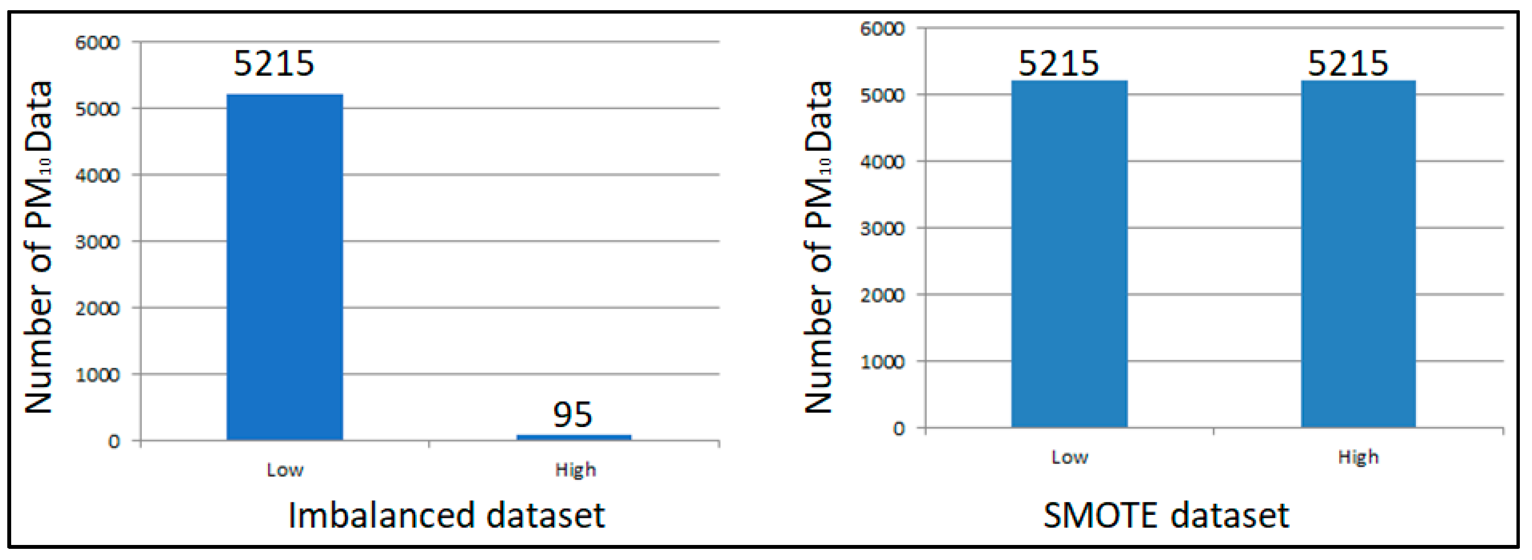
To avoid imbalanced classification in developing predictive models on these classification datasets, this study used the synthetic minority oversampling technique (SMOTE), as proposed by [39]. In the first step, the dataset was filtered to only consider the minority class, which was the high-level air quality, with 95 data points only. Following that, a search of the k-nearest neighbours was performed (k = 5). The algorithm then selected a random nearest neighbour for these data. A new data point was created, which was on the line between the two data points. The results before and after using the SMOTE technique are shown in Figure 1.

Figure 1.
Original dataset vs. synthetic minority oversampling technique (SMOTE) dataset.
2.3. Tree-Based Machine Learning Approaches
Three models were used for the prediction of PM10 concentration for the next day by using the maximum daily data in Kota Bharu, Kelantan. The models are decision trees (DTs), random forest (RF), and boosted regression trees (BRTs). In addition, in the process of model development, model prediction, and model evaluation, RapidMiner Studio was used to predict the air pollution concentration. Moreover, 80% of the data from January 2002 to December 2017 were divided into two parts, which means 80% of the data were used for training and 20% for validation of the models. Then, the results of each model were compared to find the best-proposed model for predicting PM10 concentration. Table 2 shows the general model of DT, RF, and BRT in predicting next-day PM10 concentration (PM10,D+1). The dependent variable was next-day PM10 concentration represented by PM10,D+1, while the independent variables were daily maximum CO, PM10, NO2, SO2, O3, T, RH, and WS represented by CO (D), PM10 (D), NO2 (D), SO2 (D), O3 (D), T (D), RH (D), and WS(D).

Table 2.
General model for the next day’s prediction.
2.3.1. Decision Tree
The decision tree (DT) model is a nonparametric method that can be used to predict a variety of quantitative and qualitative variables. In the form of a tree structure and with a reciprocal classification of data, a DT model illustrates direct and indirect correlations of numerous independent variables with a target variable (dependent) [40]. Variables on the upper branches of the tree structure have a greater impact on the prediction of the related class. For the DT model, four split measures were tested using gain ratio, information gain, Gini index, and accuracy.
2.3.2. Random Forests
Random forests (RFs) are a collection of methods for assembling a collection (or forest) of decision trees [41]. According to [25], the random forest (RF) approach applies the bagging technique to an ensemble of DTs, through which it trains many trees concurrently and uses the majority judgment developed in DTs as the RF model’s final decision. After that, the outputs of each tree are combined to create an ensemble prediction of the target variable. The model also estimates the most relevant features by determining how much the prediction error increases when data for that variable are permuted, while the rest of the data are not [42]. For RF models, four split measures were tested using gain ratio, information gain, Gini index, and accuracy.
2.3.3. Boosted Regression Tree
Boosted regression tree (BRT) models are developed by integrating two algorithms: Decision trees [11] are used to fit a series of single models, and then boosting [26] is used to aggregate their outputs to obtain the total prediction. A thorough description of the approaches can be found in [6,43]. The learning rate (lr), which is the shrinkage parameter used in each iteration to reduce the contribution of the tree, the complexity of the tree (tc), which is the maximum tree depth of variable interactions, as well as the number of trees (nt), are all tuning parameters that must be controlled in the BRT model. In this study, default settings for lr (0.01), tc (5), and nt (1000) were used to fit BRT models in RapidMiner. To optimise the number of trees in BRT, the optimise parameters (grid) operator was used, which is a nested operator. The loss functions or distributions that were used for this study were multinomial and Bernoulli distributions.
The DT, BRT, and RF models were run using RapidMiner software with the abovementioned independent variables (CO(D), PM10(D), NO2(D), SO2(D), O3 (D), T(D), RH(D), WS(D)) and dependent variable (PM10,D+1), with two class labels.
2.4. Performance Measures
Several performance measures—namely, accuracy, sensitivity, specificity, and precision values—were used to evaluate each classification model in this study. The formula for the performance measures used in this study is shown in Equations (1)–(4).
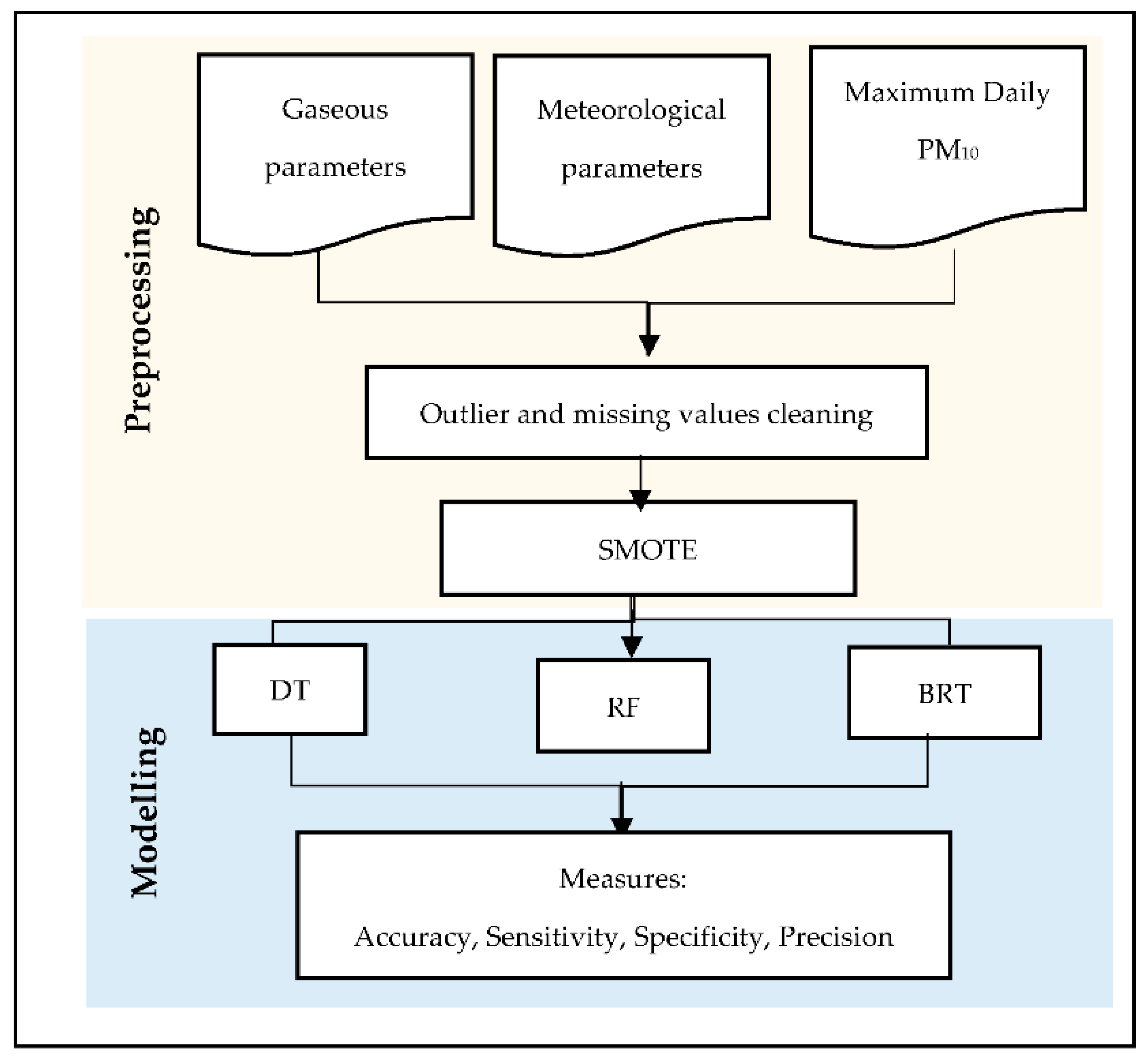
where TP is the true-positive, TN is the true-negative, FP is the false-positive, and FN is the false-negative value based on a confusion matrix. To support the accuracy values, we used sensitivity, specificity, and precision values as suggested by [44]. The overview of the experiments performed for this study is shown in Figure 2.
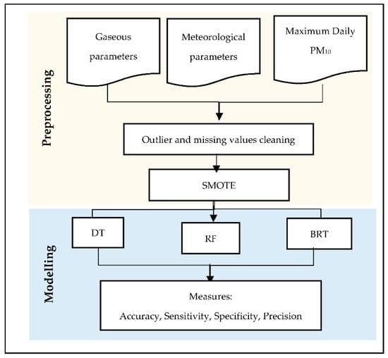
Figure 2.
Flowchart of steps in this study.
3. Results and Discussion
3.1. Statistical Characteristics of PM10
The descriptive statistics of all independent variables are shown in Table 3. The mean of the PM10 concentration was 48.73 µg/m3 below the specified MAAQG for the yearly average of 50 µg/m3 [45]. The distribution was highly skewed for PM10 (1.72), CO (16.44), NO2 (1.22), SO2 (19.54), RH (−5.92), and WS (31.08) since the values were less than −1 or more than +1 [6]. During the 2002–2017 period, the data revealed the presence of an extreme level of concentration in Kota Bharu.

Table 3.
The descriptive statistics of independent variables (IVs).
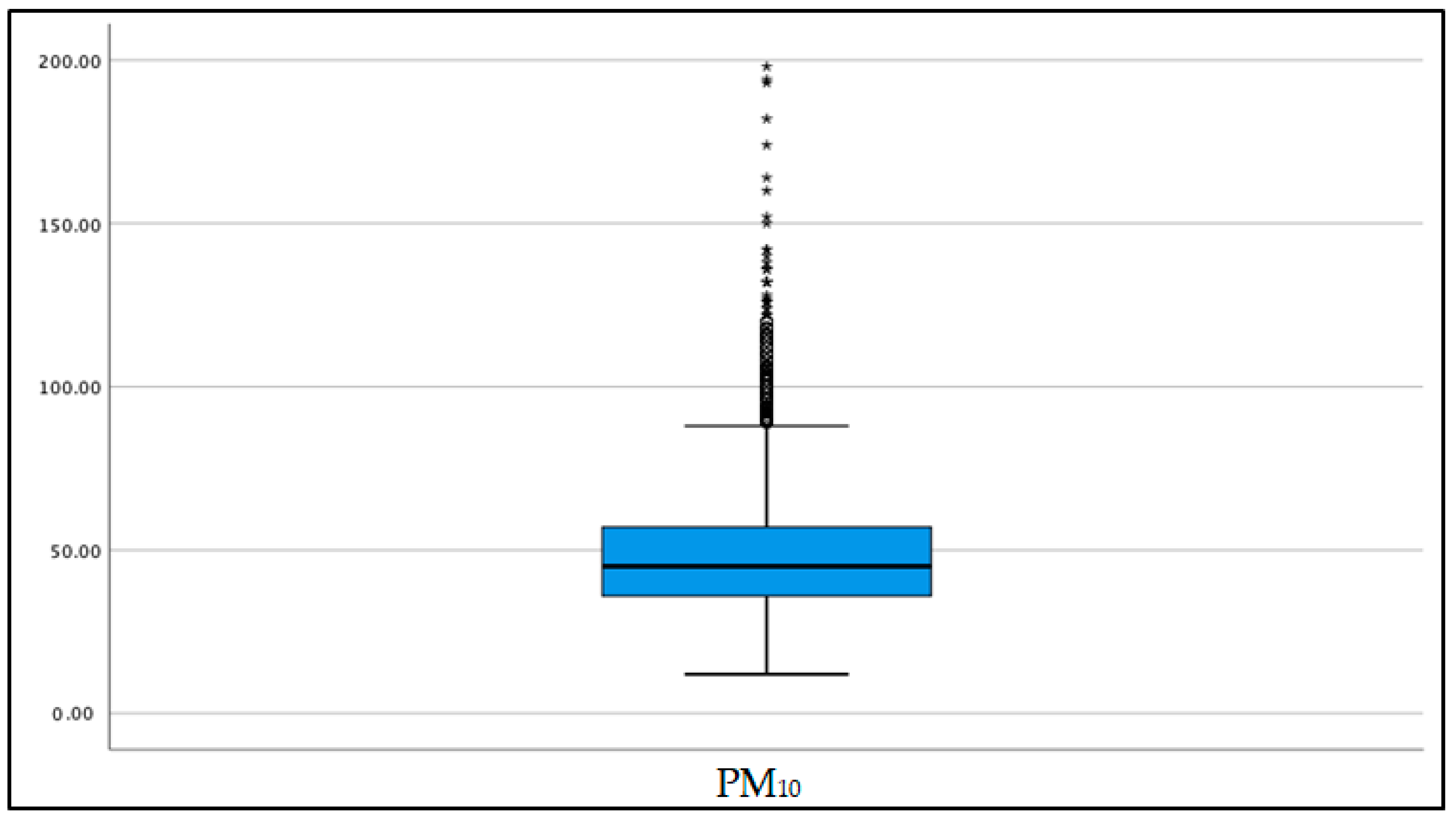
The box plot results in Figure 3 also showed that PM10 concentrations had extreme values since they consisted of many outliers. The highest extreme value indicates the maximum daily reading in 16 years of PM10 concentration. The maximum PM10 concentration was reported at 198 g/m3.

Figure 3.
Box plot for PM10 concentration.
3.2. Decision Tree (DT)
The performance values for each of the DT splitting criteria are shown in Table 4. Overall, the results indicate that all of the splitting criteria can be used to classify the air pollution dataset. On the other hand, the information gain produced the highest accuracy value in terms of total performance and recorded an impressive accuracy value of 96.52%, compared with the other splitting criteria, which was supported by sensitivity (95.78%), specificity (97.25%), and precision (97.21%).

Table 4.
The best splitting criteria for the decision tree.
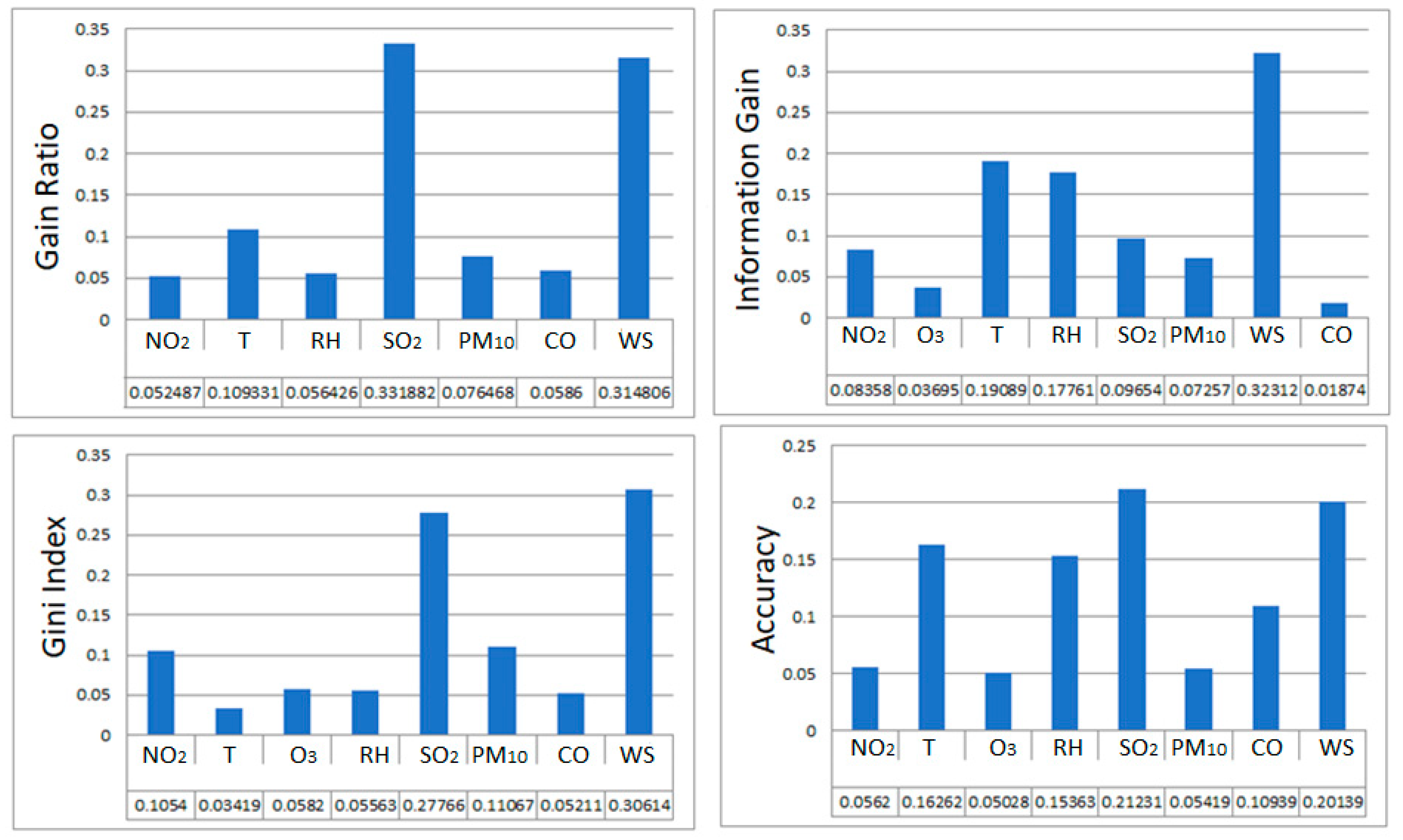
Figure 4 shows the decision tree classifier with eight features included in the model. The most influential variable regarding PM10 concentration levels was SO2 for gain ratio (0.33) and accuracy (0.21), while the second-most influential parameter would be WS for gain ratio (0.31) and accuracy (0.20). For information gain and Gini indices, the most influential variable was WS.
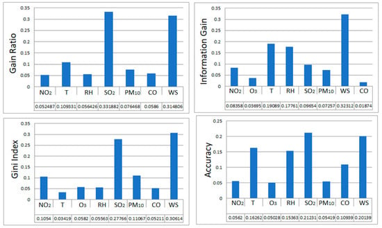
Figure 4.
Feature importance for eight parameters (decision tree (DT) model).
3.3. Boosted Regression Tree (BRT)
The performance values for each of the BRT distributions are shown in Table 5. Overall, the results indicate that both distributions can be used to classify air pollution data sets. However, the best distribution was the multinomial distribution, which had the same accuracy (98.12%) as the Bernoulli distribution but was supported by sensitivity (97.51%), specificity (98.72%), and precision (98.71%).

Table 5.
The best distribution for the boosted regression tree.
The boosted regression tree classifier, which has eight features, is shown in Figure 5. The most influential (PM10) and second-most (WS) influential variables were the same for both distributions. The parameter with the least significant influence on PM10 was ozone concentration, with only 811.43 (multinomial) and 958.16 (Bernoulli). After optimising the number of trees using the parameters (grid) operator, the best number of trees to be used in this study for multinomial was 500, and for Bernoulli, it was 450.

Figure 5.
Feature importance for eight parameters (boosted regression tree (BRT) model).
3.4. Random Forest (RF)
Table 6 shows the performance numbers for each of the RF splitting criteria. Overall, the results show that the air pollution dataset can be classified using all of the splitting criteria. In comparison to the other splitting criteria, the information gain produced the highest accuracy value in terms of total performance, with an exceptional accuracy of 98.37%, which was confirmed by sensitivity (97.19%), specificity (99.55%), and precision (99.54%).

Table 6.
The best splitting criteria for the random forest.
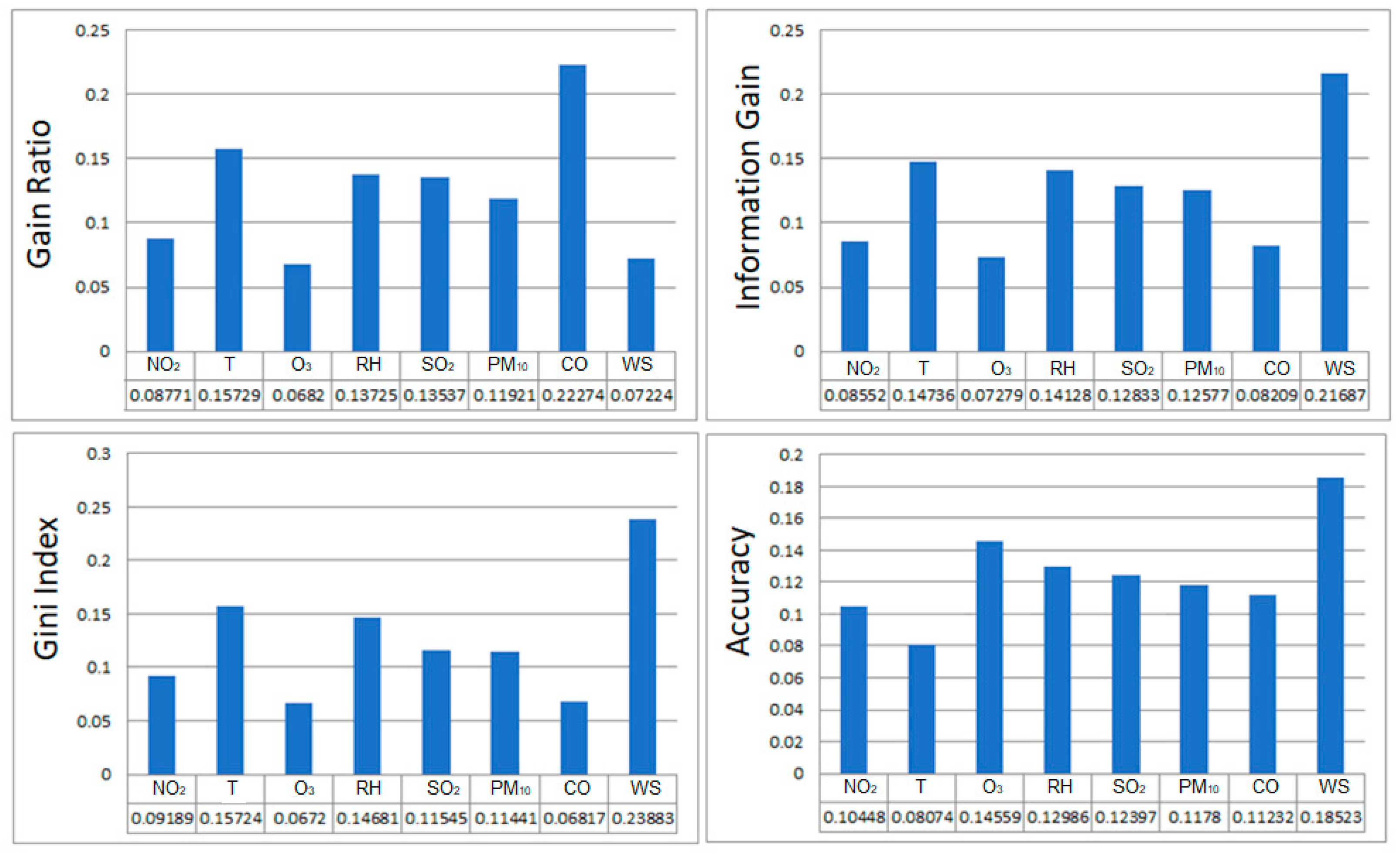
The random forest classifier, which has eight features, is shown in Figure 6. The most influential variable on PM10 concentration was WS for all methods of splitting criteria in RF, with a gain ratio of 0.22, information gain of 0.22, Gini index of 0.24, and accuracy of 0.19. The temperature was the second-most influential factor.
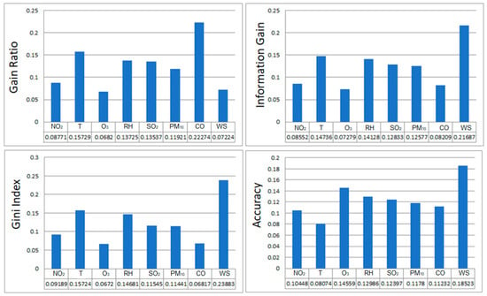
Figure 6.
Feature importance for eight parameters (random forest (RF) model).
3.5. Performance Comparison
According to the results of these performance error and accuracy measurements, the RF model outperformed BRT and DT models. As a result, in Kota Bharu, RF predicted PM10 concentrations better than BRT and DT. The values of the performance measures based on accuracy, sensitivity, specificity, and precision are shown in Table 7. Overall, the best model to use in predicting the next day’s PM10 concentration classification was the random forest classifier, with the five best parameters of WS, T, RH, NO2, and PM10. Table 8 summarises the comparison results with other researchers. The data indicate that the results in this study are quite similar to those of other researchers. In addition, the values of the accuracy are larger for the RF model, compared with those found by other models. This shows that the RF model can be used to predict PM10 concentrations since it improved the performance of the model.

Table 7.
Performance comparison for decision tree (DT), boosted regression tree (BRT), and random forest (RF).

Table 8.
Performance comparison and the results gained from other researchers.
4. Conclusions
Based on the results of this study, the random forest classifier performed the best in predicting for the next day’s PM10 concentration classification, with an accuracy of 98.37, sensitivity of 97.19, specificity of 99.55, and precision of 99.54, but the results showed that the BRT performance was not substantially different from that of the RF model, with an accuracy of 98.12, sensitivity of 97.51, specificity of 98.72, and precision of 98.71.
Next, the wind speed was the most relevant feature to classifying the next day’s PM10 concentration as indicative of a low or high level of air quality in RF and DT techniques, but for BRT, PM10 was the most relevant feature.
Overall, this study’s findings show that machine learning algorithms can help classify the next day’s PM10 concentration as indicative of a low or high level of air quality. The three classifiers applied in this research also covered the most relevant features in PM10 concentration prediction. The best model (RF) is suitable to predict PM10 concentration in Kota Bharu, Kelantan, for early warning systems and for local authorities to develop strategies to improve air quality.
The model can only be used when the sources and conditions of PM10 concentration remain constant, which is a limitation of this study. As a result, it may not be appropriate for the other areas. Furthermore, if there is a sudden forest fire or storm in a specific area, the PM10 concentration will be affected.
Author Contributions
A.Z.U.-S., W.N.S. and S.M. designed the study concept and secured funding; A.Z.U.-S. is the project administrator; W.N.S. and A.Z.U.-S. performed the data analysis; W.N.S. and S.M. wrote the manuscript; A.Z.U.-S., N.M.N. and N.S.Z. reviewed and edited the manuscript. All authors have read and agreed to the published version of the manuscript.
Funding
The research was funded by Malaysia’s Ministry of Education through the Fundamental Research Grant Scheme (FRGS/1/2019/WAB05/UITM/03/2).
Institutional Review Board Statement
Not applicable.
Informed Consent Statement
Not applicable.
Data Availability Statement
The data for this project are confidential but may be obtained with Data Use Agreements with the Department of Environment (DOE), Ministry of Environment and Water of Malaysia.
Acknowledgments
The authors thank Universiti Teknologi MARA for their support and also the Department of Environment Malaysia for providing air quality monitoring data.
Conflicts of Interest
The authors declare no conflict of interest. The funders had no role in the design of the study; in the collection, analyses, or interpretation of data; in the writing of the manuscript; in the decision to publish the results.
References
- Department of Environment, Malaysia. Malaysia Environmental Quality Report 2016. Available online: https://www.doe.gov.my/wp-content/uploads/2021/08/EQR-2016-AIR-TANAH.pdf (accessed on 1 January 2022).
- US EPA. Health and Environmental Effects of Particulate Matter (PM) 2015. Available online: https://www.epa.gov/pm-pollution/health-and-environmental-effects-particulate-matter-pm (accessed on 4 January 2022).
- Hassan, N.A.; Hashim, Z.; Hashim, J.H. Impact of climate change on air quality and public health in urban areas. Asia Pac. J. Public Health 2016, 28, 385–485. [Google Scholar] [CrossRef]
- Vinceti, M.; Malagoli, C.; Malavolti, M.; Cherubini, A.; Maffeis, G.; Rodolfi, R.; Heck, J.E.; Astolfi, G.; Calzolari, E.; Nicolini, F. Does maternal exposure to benzene and PM10 during pregnancy increase the risk of congenital anomalies? A population-based case-control study. Sci. Total Environ. 2016, 541, 444–450. [Google Scholar] [CrossRef] [PubMed] [Green Version]
- Azmi, S.Z.; Latif, M.T.; Ismail, A.S.; Juneng, L.; Jemain, A.A. Trend and status of air quality at three different monitoring stations in the Klang Valley, Malaysia. Air Qual. Atmos. Health 2010, 3, 53–64. [Google Scholar] [CrossRef] [PubMed] [Green Version]
- Shaziayani, W.N.; Ul-Saufie, A.Z.; Ahmat, H.; Al-Jumeily, D. Coupling of Quantile Regression into Boosted Regression Trees (BRT) Technique in Forecasting Emission Model of PM10 Concentration. Air Qual. Atmos. Health 2021, 14, 1647–1663. [Google Scholar] [CrossRef]
- Byun, D.; Schere, K.L. Review of the governing equations, computational algorithms, and other components of the Models-3 Community Multiscale Air Quality (CMAQ) modeling system. Appl. Mech. Rev. 2006, 59, 51–77. [Google Scholar] [CrossRef]
- Im, U.; Markakis, K.; Unal, A.; Kindap, T.; Poupkou, A.; Incecik, S.; Yenigun, O.; Melas, D.; Theodosi, C.; Mihalopoulos, N. Study of a winter PM episode in Istanbul using the high resolution WRF/CMAQ modeling system. Atmos. Environ. 2010, 44, 3085–3094. [Google Scholar] [CrossRef]
- Hu, J.; Li, X.; Huang, L.; Ying, Q.; Zhang, Q.; Zhao, B.; Wang, S.; Zhang, H. Ensemble prediction of air quality using the WRF/CMAQ model system for health effect studies in China. Atmos. Chem. Phys. 2017, 17, 13103–13118. [Google Scholar] [CrossRef] [Green Version]
- Vongruang, P.; Wongwises, P.; Pimonsree, S. Assessment of fire emission inventories for simulating particulate matter in Upper Southeast Asia using WRF-CMAQ. Atmos. Pollut. Res. 2017, 8, 921–929. [Google Scholar] [CrossRef]
- Tan, J.; Zhang, Y.; Ma, W.; Yu, Q.; Wang, Q.; Fu, Q.; Zhou, B.; Chen, J.; Chen, L. Evaluation and potential improvements of WRF/CMAQ in simulating multi-levels air pollution in megacity Shanghai, China. Stoch. Environ. Res. Risk Assess. 2017, 31, 2513–2526. [Google Scholar] [CrossRef]
- Zhang, H.; DeNero, S.P.; Joe, D.K.; Lee, H.H.; Chen, S.H.; Michalakes, J.; Kleeman, M.J. Development of a source oriented version of the WRF/Chem model and its application to the California regional PM 10/PM 2.5 air quality study. Atmos. Chem. Phys. 2014, 14, 485–503. [Google Scholar] [CrossRef] [Green Version]
- Kumar, A.; Jime, R.; Belalca, L.C. Application of WRF-Chem model to simulate PM10 concentration over Bogota. Aerosol Air Qual. Res. 2016, 16, 1206–1221. [Google Scholar] [CrossRef] [Green Version]
- Jenkins, G.S.; Gueye, M. Annual and early summer variability in WRF-CHEM simulated West African PM10 during 1960–2016. Atmos. Environ. 2022, 273, 118957. [Google Scholar] [CrossRef]
- Casallas, A.; Celis, N.; Ferro, C.; López Barrera, E.; Peña, C.; Corredor, J.; Ballen Segura, M. Validation of PM10 and PM2.5 early alert in Bogotá, Colombia, through the modeling software WRF-CHEM. Environ. Sci. Pollut. Res. 2020, 27, 35930–35940. [Google Scholar] [CrossRef] [PubMed]
- Grell, G.A.; Peckham, S.E.; Schmitz, R.; McKeen, S.A.; Frost, G.; Skamarock, W.C.; Eder, B. Fully coupled “online” chemistry within the WRF model. Atmos. Environ. 2005, 39, 6957–6975. [Google Scholar] [CrossRef]
- Balzarini, A.; Pirovano, G.; Honzak, L.; Žabkar, R.; Curci, G.; Forkel, R.; Hirtl, M.; San Jose, R.; Tuccella, P.; Grell, G.A. WRF-Chem model sensitivity to chemical mechanisms choice in reconstructing aerosol optical properties. Atmos. Environ. 2015, 115, 604–619. [Google Scholar] [CrossRef]
- Gagliardi, R.V.; Andenna, C. A Machine Learning Approach to Investigate the Surface Ozone Behavior. Atmosphere 2020, 11, 1173. [Google Scholar] [CrossRef]
- Rybarczyk, Y.; Zalakeviciute, R. Machine Learning Approaches for Outdoor Air Quality Modelling: A Systematic Review. Appl. Sci. 2018, 8, 2570. [Google Scholar] [CrossRef] [Green Version]
- Myers, K.D.; Knowles, J.W.; Staszak, D.; Shapiro, M.D.; Howard, W.; Yadava, M.; Zuzick, D.; Williamson, L.; Shah, N.H.; Banda, J.M.; et al. Precision screening for familial hypercholesterolaemia: A machine learning study applied to electronic health encounter data. Lancet Digit. Heal. 2019, 1, 393–402. [Google Scholar] [CrossRef] [Green Version]
- Rosli, M.M.; Edward, J.; Onn, M.; Chua, Y.A.; Kasim, N.A.M.; Nawawi, H. Classifying Familial Hypercholesterolaemia: A Tree-based Machine Learning Approach. Int. J. Adv. Comput. Sci. Appl. 2021, 12, 66–73. [Google Scholar] [CrossRef]
- Breiman, L.; Friedman, J.H.; Olshen, R.; Stone, C.J. Classification and Regression Trees; Wadsworth: Belmont, CA, USA, 1984. [Google Scholar]
- Quinlan, R. C4.5: Programs for Machine Learning; Morgan Kaufmann: San Mateo, CA, USA, 1993. [Google Scholar]
- Hastie, T.; Tibshirani, R.; Friedman, J.H. The Elements of Statistical Learning: Data Mining, Inference, and Prediction; Springer: New York, NY, USA, 2009. [Google Scholar]
- Breiman, L. Random forests. Mach. Learn. 2001, 45, 5–32. [Google Scholar] [CrossRef] [Green Version]
- Friedman, J.H. Greedy function approximation: A gradient boosting machine. Ann. Stat. 2001, 29, 1189–1232. [Google Scholar] [CrossRef]
- Friedman, J.H. Stochastic gradient boosting. Comput. Stat. Data Anal. 2002, 38, 367–378. [Google Scholar] [CrossRef]
- Elith, J.; Leathwick, J.R.; Hastie, T. A Working Guide to Boosted Regression Trees. J. Anim. Ecol. 2008, 77, 802–813. [Google Scholar] [CrossRef] [PubMed]
- Akiladevi, R.; Nandhini, D.B.; Nivesh, K.V.; Nivetha, P. Prediction and Analysis of Pollutant using Supervised Machine Learning. Int. J. Recent Technol. Eng. 2020, 9, 50–54. [Google Scholar]
- Giorgio, C.; Mauro, S. Air pollution prediction via multi-label classification. Environ. Model. Softw. 2016, 80, 259–264. [Google Scholar]
- Akhtar, A.; Masood, S.; Gupta, C.; Masood, A. Prediction and analysis of pollution levels in delhi using multilayer perceptron. Adv. Intell. Syst. Comput. 2018, 542, 563–572. [Google Scholar]
- Grivas, G.; Chaloulakou, A. Artificial neural network models for prediction of PM10 hourly concentrations, in the Greater Area of Athens, Greece. Atmos. Environ. 2006, 40, 1216–1229. [Google Scholar] [CrossRef]
- Elis, S.Z.N.; Ul-Saufie, A.Z.; Shaziayani, W.N.; Noor, N.M.; Zubir, N.A. Assessment of Ambient Air Pollution in Langkawi Island, Malaysia. In Proceedings of the IOP Conference Series: Materials Science and Engineering, Kazimierz Dolny, Poland, 21–23 November 2019; Volume 551, p. 012123. [Google Scholar]
- Mohamad, N.S.; Deni, S.M.; Ul-Saufie, A.Z. Application of the First Order of Markov Chain Model in Describing the PM10 Occurrences in Shah Alam and Jerantut, Malaysia. Pertanika J. Sci. Technol. 2018, 26, 367–378. [Google Scholar]
- Paschalidou, A.K.; Karakitsios, S.; Kleanthous, S.; Kassomenos, P.A. Hourly PM10 Concentration in Cyprus through Artificial Neural Networks and Multiple Regression Models: Implications to Local Environmental Management. Environ. Sci. Pollut. Res. 2011, 18, 316–327. [Google Scholar] [CrossRef] [PubMed]
- Papanastasiou, D.K.; Kioutsoukis, M.D. Development And Assessment Of Neural Network And Multiple Regression Models In Order To Predict PM10 Levels In A Medium-Sized Mediterranean City. Water Air Soil Pollut. 2007, 182, 325–334. [Google Scholar] [CrossRef]
- Libasin, Z.; Suhailah, W.; Fauzi, W.M.; Ul-Saufie, A.Z.; Idris, N.A.; Mazeni, N.A. Evaluation of Single Missing Value Imputation Techniques for Incomplete Air Particulates Matter (PM10) Data in Malaysia. Pertanika J. Sci. Technol. 2021, 29, 3099–3112. [Google Scholar] [CrossRef]
- Department of Environment, Malaysia. Malaysia Environmental Quality Report 2019. Available online: https://www.doe.gov.my/portalv1/en/ (accessed on 10 January 2022).
- Chawla, N.V.; Bowyer, K.W.; Hall, L.O.; Kegelmeyer, W.P. SMOTE: Synthetic Minority Over-sampling Technique. J. Artif. Intell. Res. 2002, 16, 321–357. [Google Scholar] [CrossRef]
- Esfandiarpour-Boroujeni, I.; Shahini, S.M.; Shirani, H.; Mosleh, Z.; Bagheri, B.M.; Salehi, M.H. Comparison of error and uncertainty of decision tree and learning vector quantization models for predicting soil classes in areas with low altitude variations. CATENA 2020, 191, 104581. [Google Scholar] [CrossRef]
- Stafoggia, M.; Bellander, T.; Bucci, S.; Davoli, M.; Hoogh, K.D.; Donato, F.D.; Gariazzo, C.; Lyapustin, A.; Michelozzi, P.; Renzi, M.; et al. Estimation of daily PM10 and PM2.5 concentrations in Italy, 2013–2015, using a spatiotemporal land-use random-forest model. Environ. Int. 2019, 124, 170–179. [Google Scholar] [CrossRef] [PubMed]
- Liaw, A.; Wiener, M. Classification and regression by random forest. R News 2002, 2, 18–22. [Google Scholar]
- Shaziayani, W.N.; Ul-Saufie, A.Z.; Yusoff, S.A.M.; Ahmat, H.; Libasin, Z. Evaluation of boosted regression tree for the prediction of the maximum 24-hour concentration of particulate matter. Int. J. Environ. Sci. Dev. 2021, 12, 126–130. [Google Scholar] [CrossRef]
- Rosli, M.M.; Edward, J.; Onn, M. Precision screening for familial hypercholesterolaemia: A machine learning study applied to electronic health encounter data. Int. J. Adv. Comput. Sci. Appl. 2021, 9, 66–73. [Google Scholar]
- Department of Environment, Malaysia. Malaysia Environmental Quality Report 2018; Ministry of Energy, Science, Technology, Environment and Climate Change, Malaysia: Kuala Lumpur, Malaysia, 2018.
Publisher’s Note: MDPI stays neutral with regard to jurisdictional claims in published maps and institutional affiliations. |
© 2022 by the authors. Licensee MDPI, Basel, Switzerland. This article is an open access article distributed under the terms and conditions of the Creative Commons Attribution (CC BY) license (https://creativecommons.org/licenses/by/4.0/).

