Article

Joint Distribution Analysis of Forest Fires and Precipitation in Response to ENSO, IOD, and MJO (Study Case: Sumatra, Indonesia)

by
Sri Nurdiati
1,*,
Ardhasena Sopaheluwakan
2 and
Pandu Septiawan
1
1
Department of Mathematics, Mathematics and Natural Science Faculty, IPB University, Bogor 16680, Indonesia
2
Center for Applied Climate Services, Agency for Meteorology Climatology and Geophysics, Jakarta 10720, Indonesia
*
Author to whom correspondence should be addressed.
Atmosphere 2022, 13(4), 537; https://doi.org/10.3390/atmos13040537
Submission received: 1 March 2022 / Revised: 25 March 2022 / Accepted: 26 March 2022 / Published: 28 March 2022

Abstract

:
To evaluate the impact of the El Niño Southern Oscillation (ENSO), Indian Ocean Dipole (IOD), and Madden Julian Oscillation (MJO) on the occurrence of land and forest fire in Sumatra, copula-based joint distribution analysis and quadrant analysis (for extreme events) were carried out in this research. This research used dry spells (number of days without rain) and precipitation anomalies as climate indicators and hotspots as land and forest fire indicators. Using data spanning from 2001 to 2020, this research shows that ENSO and IOD strongly influence hotspots in Sumatra with monsoonal-type precipitation. Even though the impact is not linear, the probability of a higher number of hotspots occurring increases significantly, especially during strong El Niño and weak El Niño combined with positive IOD. Furthermore, the results show that moderate El Niño has a similar impact to weak El Niño on the affected area, while weak El Niño combined with positive IOD can result in effects similar to robust El Niño impact. Meanwhile, this research has shown that the MJO affects hotspots in the first dry season of Sumatran areas that have equatorial-type precipitation. Although its impact on dry spell–precipitation anomaly dependency is unclear, phases 6,7, and 8 of MJO significantly increase dry spell–hotspot dependency during dry conditions.

1. Introduction

As the global average temperature increases (global warming), some researchers point out that the variability and occurrence of extreme climates have increased in recent decades [1,2,3]. If the trend continues, there is the potential for more significant fires to occur in the future [4]. Land and forest fires are annual phenomena that occur on the island of Sumatra. Due to the limited amount of historical data, analysis of the multivariate distribution of forest and climate indicators is needed to assist the government in predicting land and forest fires in Sumatra with the impact of future extreme climates. In 2013, research in [5] revealed that land and forest fires on Sumatra are divided into two types following the seasonal precipitation pattern in each region. The rainy season patterns are monsoonal and equatorial [6]. The monsoonal rain pattern is a rain pattern with a period of 12 months, with the dry season occurring around June–August. Meanwhile, the equatorial rain pattern is a rain pattern with two peaks of dry season in a year, namely around March and October, so it has a rainy season period of six months. The pattern of land and forest fires related to the monsoonal pattern occurs in the South Sumatra region and its surroundings, while the land and forest fires in the equatorial pattern occur in the Riau region and its surroundings [5]. Land and forest fire characteristics are reflected in the shared pattern of forest and land fire indicators and rainfall in the area [7,8].
Research in [7] explains the relationship between indicators of burnt area, carbon emissions, and rainfall together using principal component analysis. The study shows that the burned area has a closer relationship with rainfall when compared to carbon emissions as a climate indicator. The monsoonal forest and land fire patterns have a period of 12 months, while the equatorial forest fire pattern has a period of 6 months [7]. However, the contribution of the equatorial forest and land fire patterns to the overall data (annual signal) is very small when compared to the monsoonal one. If the pre-processing data is not carried out properly (without separating the analyzed area that doesn’t have an equatorial signal), the equatorial fire pattern may not be detected [8].
Besides being influenced by these two types of rain, the variation of precipitation (extreme high/low precipitation) in Sumatra is influenced by global climate phenomena, namely El Niño Southern Oscillation (ENSO) and the Indian Ocean Dipole (IOD) [9]. ENSO is an anomalous event in which sea surface temperatures in the Pacific Ocean on the west coast of Ecuador and Peru are higher than the normal average. ENSO has two phases, namely La Niña and El Niño [10]. The impact of El Niño on Indonesia is that there is a decrease in the intensity of rainfall with a delay in the onset of the rainy season in Indonesia [9], leading to a more severe dry season. Meanwhile, IOD is a phenomenon of oscillation of sea surface temperature in the western Indian Ocean, which is warmer (in the positive phase) and cooler (in the negative phase) than the eastern region of the Indian Ocean on an irregular basis [11]. Of the two phases, positive IOD is a phenomenon that can reduce precipitation around west IOD SST (50° E to 70° E and 10° S to 10° N) as well as increase the severity of the dry season in the southern part of Sumatra when occurring during the dry season [9]. Therefore, the increased severity of southern Sumatra’s dry season becomes more significant when El Niño and positive IOD occur in the same period.
In 2021, research in [12] showed that El Niño and positive IOD also had a positive correlation with land and forest fires in Sumatra. This is evidenced by the increasing scale and duration of the forest and land fire phenomena when they occur together with El Niño and/or positive IOD [13]. Research in [13] also explains that the increase in the scale of the land and forest fire phenomenon that occurs is not linear with the increasing strength of El Niño and/or IOD, and not all land and forest fires in Sumatra are affected by El Niño and/or IOD. The land and forest fires that have a strong correlation with El Niño and IOD are land and forest fires that occur in areas with monsoonal rain types [12]. For instance, land and forest fires that occur in the Riau region are not affected by this phenomenon [13]. This nonlinearity is supported by research that transforms the Niño3.4 and DMI indexes into a new value that correlates with ENSO and IOD impact on the region following the general logistic function [14]. With this step, the correlation of the Niño3.4 index and DMI to the number of hotspots in the southern Sumatra region (monsoon rain type) increase. Not only does the index transformation process increase the correlation, but it also significantly increases the performance of the regression model built in this study.
Although not significantly affected by the El Niño phenomenon and positive IOD, land and forest fires in the Riau region can increase drastically, as seen in 2013 and 2014. One of the phenomena that has an influence on increasing drought in that period is the Madden–Julian Oscillation (MJO) [15]. The MJO is a 40–50-day oscillatory phenomenon that occurs in the tropics that can suppress the mean sea level pressure, causing convection in the tropics, especially in the Indonesian maritime region [16]. Although it has a short duration and a small effect, several researchers have shown that the MJO has an influence on rainfall in Riau and surrounding areas [17,18,19]. Although not on the same scale or lasting as long as ENSO and IOD, extreme MJO phenomena can cause severe droughts, which resulted in over 6000 fires per month in 2014 [13]. However, there is no research that directly discusses the relationship between the MJO phenomenon and land and forest fires in the Sumatra region with the equatorial type of rainfall (Riau and its surroundings). The results of this study can explain how ENSO, IOD, and MJO affect land and forest fires in Sumatra, as well as contribute positively to modeling predictions of land and forest fires in the future. This is in line with one of the focus areas or strategic plans of global research, namely disaster and climate change mitigation.

2. Materials and Methods

This research uses daily CPC MORPHing technique (CMORPH) precipitation data which have a spatial resolution of 0.25° × 0.25° [20]. According to previous research, CMORPH data outperformed other datasets such as Climate Hazards Group InfraRed Precipitation with Station data (CHIRPHS), ERA5, etc., in terms of accuracy and rainfall detection capability at the daily scale [21]. After that, we derived the data to obtain the monthly dry spell (the number of days without rain) and precipitation anomaly, which contained information from the last three months (accumulation of dry spell and average of precipitation anomaly). The temporal resolution of data used is from November 2000 until December 2020, following the availability of MODIS NRT hotspot data. The hotspot data were obtained from MODIS NRT active fire products obtained from NASA Earth data [22]. The analysis was done on Sumatra Island data from 95° E–107° E and 6° S–6° N. The MJO index was obtained from the Bureau of Meteorology, Australia, while the ENSO and IOD classifications were provided by the Golden Gate Weather Service (GGWS) website based on the Oceanic Niño Index (ONI), which calculates the running mean of 3 months of SST anomaly from the Nino3.4 region. Since land and forest fire events in Sumatra happened around every 2–3 months [13], the range of dry spells is around 0 to 90 s. We assume that the ONI-based categorization at least covered the 3 months without rain.
The methods that were used in this research are bivariate analyses based on copulas. Using the copula approach, this research analyzes the dependency between dry spell–precipitation anomaly, dry spell–hotspot, and precipitation anomaly–hotspot. The analysis was divided into two main sections, which cover locations with monsoonal-type precipitation as well as equatorial-type precipitation, as shown in Figure 1. Figure 1 was a representation of the 2nd mode as a result of singular value decomposition (SVD) of monthly precipitation data from 2001–2020, following previous research [6]. The 2nd mode of SVD is a vector with length 1 and captures precipitation signal, which has around a 6-month period (equatorial-type precipitation). Therefore, positive values represent areas that have equatorial-type precipitation. Meanwhile, negative values represent areas that only have monsoonal-type precipitation.
In order to obtain the best univariate distribution that fits the observed data, this research uses the “MATLAB Fitmethis function” [23]. The package finds the distribution that best fits data in vector X among all distributions available in MATLAB using a maximum likelihood estimation (MLE) function, which can be learned about in [24]. From the fitting process, we obtain the Rayleigh distribution as a hotspot distribution and the generalized extreme value (GEV) as dry spell and precipitation anomaly distribution. For random variable x , the probability density function of Rayleigh [25], followed by GEV [26], is:
y = f ( x | b ) = x b 2 e x 2 2 b 2 ,   where   b   is   shape   parameter ,
y = f ( x   |   k ,   μ ,   σ ) = ( 1 σ ) exp ( ( 1 + k ( x μ ) σ ) 1 k ) ( 1 + k ( x μ ) σ ) 1 1 k ,
where μ is location parameter, σ is scale parameter, and k 0 is shape parameter.
For the bivariate variable pair, we use the MATLAB Copula repository [27]. Using those two distributions as a base, there are four copula families that emerge as the family’s best that correspond to the corresponding conditions, which are Gaussian, Clayton, Frank, Gumbel, and t. Before that, we measure the association inspired by Spearman’s rho of each pair ( X , Y ) of variables (dry spell–anomaly, dry spell–hotspot, and anomaly–hotspot), following the equation from [28] below:
ρ [ X , Y ] = c o v ( F ( X ) , G ( Y ) ) v a r ( F ( X ) )   v a r ( G ( Y ) )
The cumulative distribution function for each family is shown in Table 1 [29,30,31]. The parameter and dependence parameter of the copula itself are calculated using maximum likelihood estimation, following research from [32] and the equation below:
θ n = a r g θ max l ( θ ) l ( θ ) = i = 1 n log c { F 1 ( y i 1 ) , , F d ( y i d ) } + i = 1 n j = 1 d l o g f j ( y i j )
We used the Akaike Information Criterion (AIC) parameter as suggested by [32] to choose the copula function. AIC, as derived in [33], is defined as
A I C = 2   ( m a x i m u m log l i k e l i h o o d ) + 2 ( n u m b e r   o f   f r e e   p a r a m e t e r ) A I C = 2 l ( θ n ) + 2 q
where l ( θ n ) is the maximized value of the log likelihood function l ( θ ) defined in Equation (4) and q is the number of free parameters. After that, we calculate the survival conditional probability from the survival conditional distribution from each pair of variables, which represents the probability of a certain extreme condition happening. Following research in [34], we denote ( X , Y ) as a random variable pair with bivariate cumulative distribution F X , Y and continuous marginal c.d.f’s F X and F Y , respectively. For any 0 u , v 1 , the copula of ( X , Y ) is given by
C ( u , v ) = F X , Y ( F X 1 ( u ) , F Y 1 ( v ) )
where F X 1 and F Y 1 are the marginal quantile function. C * is called the survival copula of ( X , Y ) , or dual copula, and is related to copula C by
C * ( u , v ) = 1 u v + C ( 1 u , 1 v )
The survival distribution of ( X , Y ) is given by
F ¯ X , Y ( x , y ) = ( X > x , Y > y ) = C * ( F ¯ X ( x ) , F ¯ Y ( y ) )
where F ¯ X ( x ) = P ( X < x ) , and F ¯ Y ( y ) = P ( Y < y ) . Using Equation (8), the conditional survival distribution could be obtained from joint and marginal survival distributions. For any F ¯ X ( x ) , F ¯ Y ( y ) [ 0 , 1 ] , the conditional survival distribution of X given Y > y is
G ¯ ( C , x , y ) = ( X > x   | Y > y ) = ( X > x , Y > y ) ( Y > y ) = C * ( F ¯ X ( x ) , F ¯ Y ( y ) ) 1 F ¯ Y ( y )
Moreover, this research also uses the quadrant analysis concept [34,35,36,37] to gain more insight into the tail of the distribution, which represents the most extreme events from 2001 to 2020.

3. Results

3.1. Sumatra with Monsoonal-Type Precipitation

The southern Sumatra region, which has monsoonal-type precipitation, often suffers from land and forest fires, specifically around Palembang [38]. Many researchers show that fire events in these areas were highly related to El Niño followed by positive IOD [13,39,40,41,42]. Therefore, analysis in this region was separated in order to get a more in-depth result with respect to the strength of El Niño and positive IOD. The separation is the classification produced by GGWS the following year based on ONI, with some adjustments to correspond to the dry season, namely:
  • La Niña (LaN): 2005, 2007, 2008, 2010, 2011, 2016, and 2017.
  • Normal year: 2001, 2003, 2012, 2013, 2018, and 2020.
  • Weak El Niño (WEN): 2004 and 2014.
  • Moderate El Niño (MEN): 2002 and 2009.
  • Strong El Niño (SEN): 2015.
  • Weak El Niño, positive IOD (WENPI): 2006 and 2019.
Unfortunately, there are only 2 years that represent weak and moderate El Niño, as well as positive IOD during a weak El Niño. Even more, there is only one event that represents a strong El Niño event. Although the result of this research might not be able to describe all possible events (such as the forest fire anomaly in 1997), the result can still be used to describe the general description of the event based on data from 2001 to 2020. Due to the focus of this research being to analyze the forest fire event, the analysis was only carried out on data that represented the dry season (June–November).

3.1.1. Dependency between Pair of Two Variables

The measures of association between the empirical data on Table 2 are calculated using Equation (3). The result represents the association of the empirical data from each variable pair in respective year categories. The positive value represents that paired variable have a positive relation to each other, so increasing the value of one variable will also increase the value of the paired variable. Meanwhile, the negative value shows the opposite direction of paired variables responding to each other. The strength of the association is obtained by ignoring the positive/negative values of the association. Obviously, the association of hotspot with other variable in LaN category is irrelevant due to the lack of land and forest fire events during the year. From the analysis, we can see that the association of dry spell–prec. anomaly and dry spell–hotspot increases starting from normal until the WENPI category. Meanwhile, prec. anomaly did not show consistent change in response to the year category. This result shows that in general (not based on a specific variable’s value), dry spell is more affected by the ENSO and IOD than precipitation anomaly. Therefore, a better representation of ENSO and IOD impact on hotspots will be achieved when using dry spell indicator.
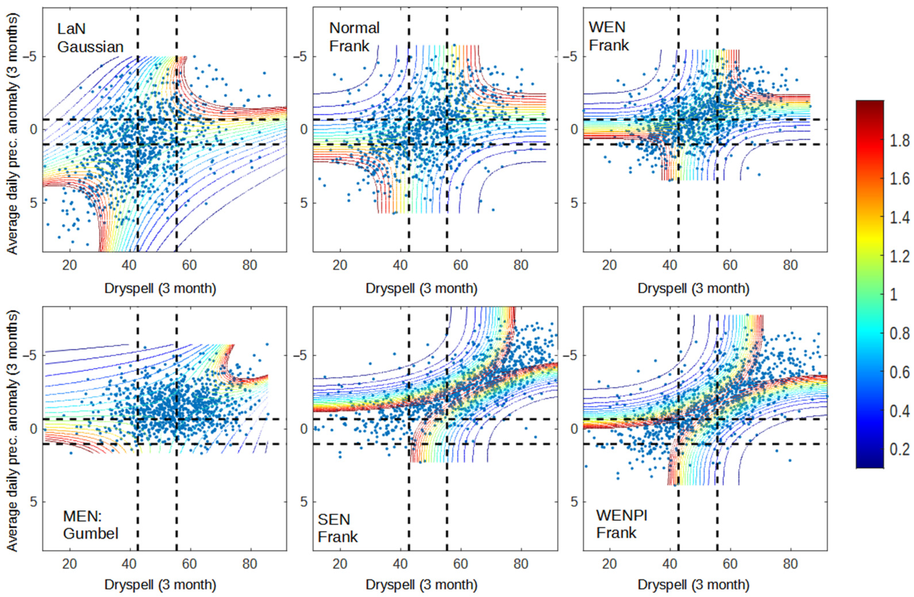
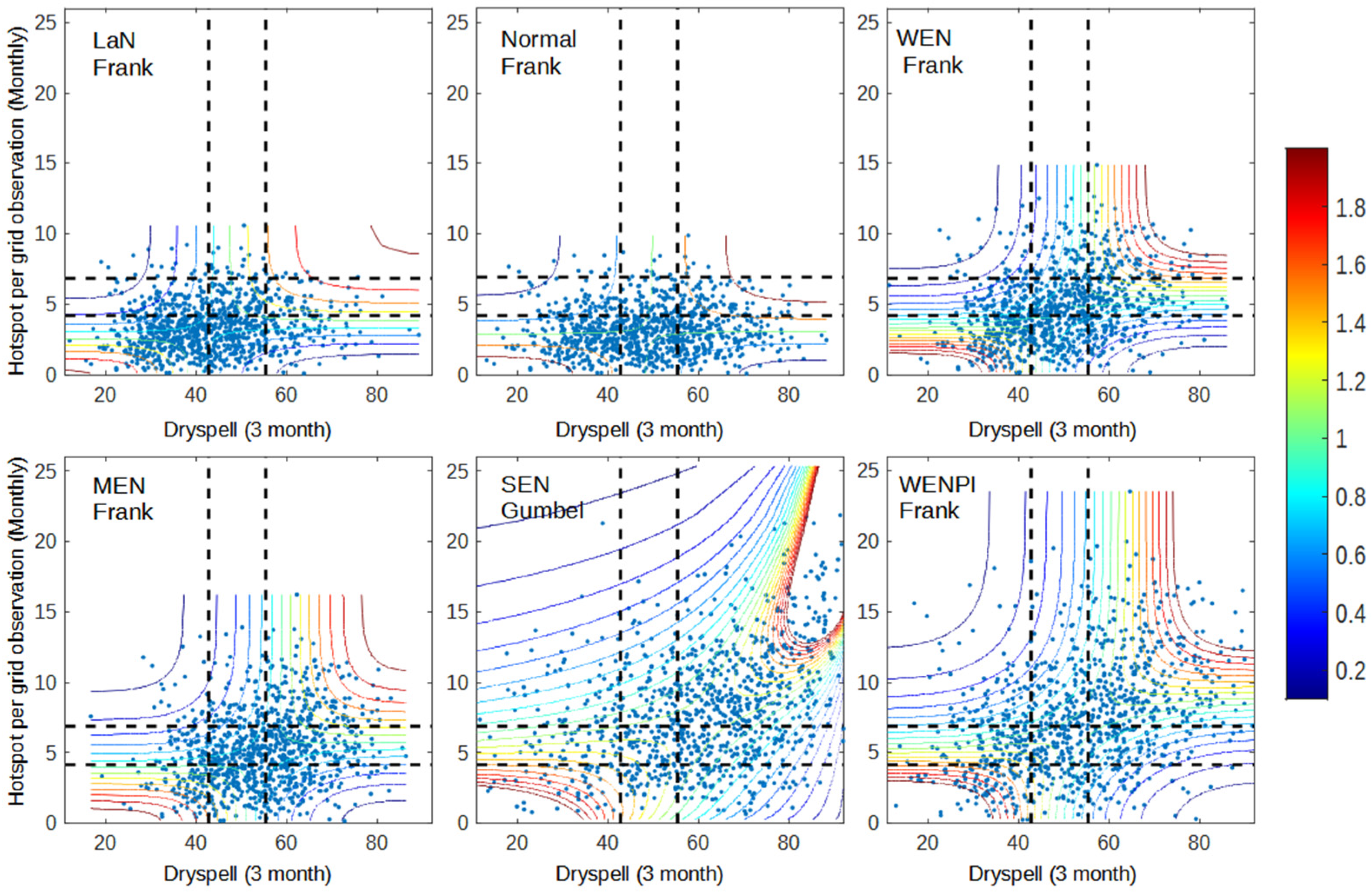
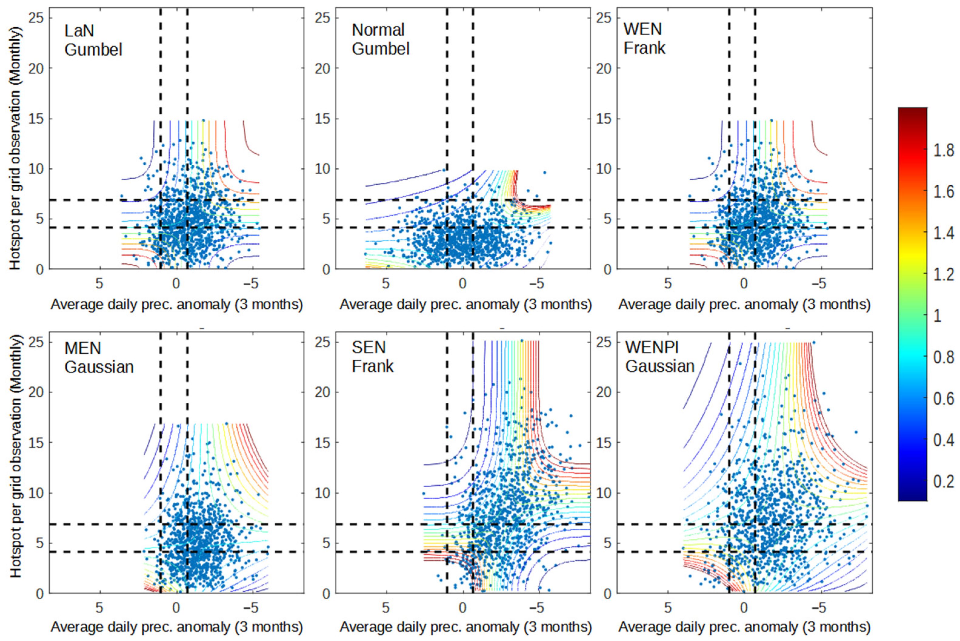
Figure 1, Figure 2 and Figure 3 shows the dependency between pairs of each variable (dry spell–anomaly, dry spell–hotspot, and anomaly–hotspot). The dependency is calculated using the joint probability of each respective copula from the copula analysis. Pairs of x and y values have a higher probability of occurrence when the pair has a high dependency value when compared to those with low dependency. Furthermore, when x and y have high dependency, the value of y is easier to model if we know the value of x, and vice versa. The results that were obtained from the dependency analysis were as good as expected, where areas in the range of wet–wet, normal–normal, and dry–dry had higher dependency than other areas. This is caused by the behavior of all variables during the dry season, where precipitation anomaly decreases while dry spell and hotspot are increased. As a result, the likelihood of variable pair values occurring under wet–dry or dry–wet conditions are low. Even though all variables behave in the same direction, the way each pair behaves in response to ENSO and IOD conditions is different.
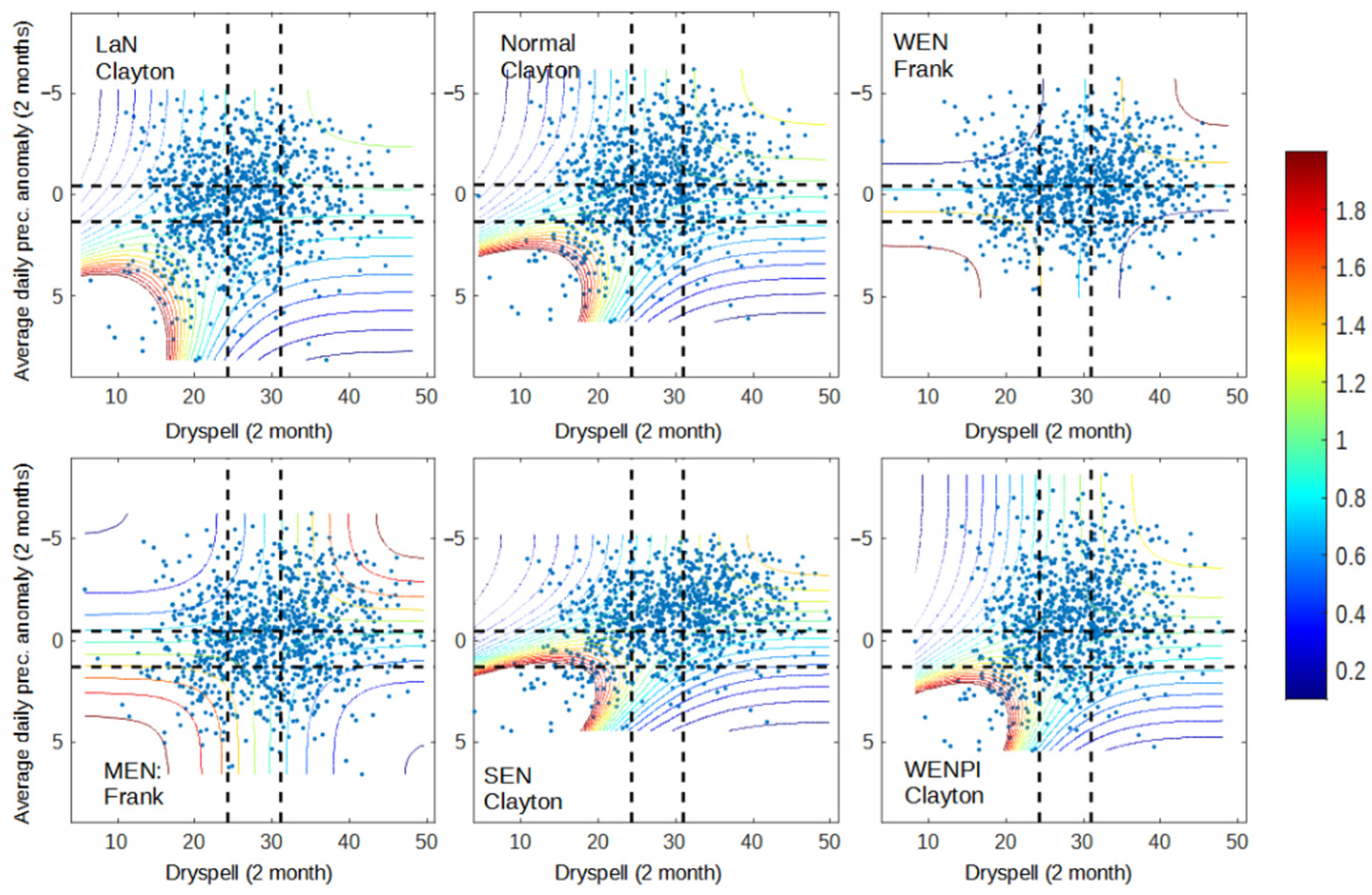
Figure 1 shows that precipitation anomalies in Sumatra with monsoonal-type precipitation are more responsive to the occurrence of El Niño and positive IOD, especially in wet conditions. This result is shown by the number of data points in wet–wet conditions (bottom-left) from each year category, which has a decreasing trend following the strength of El Niño. During moderate and strong El Niño, almost all of the data points are above the wet condition of the precipitation anomaly. Meanwhile, there are still many data points that are on the left side of the dry spell wet condition, even on the MEN and SEN graphs (Figure 1). During a normal year, 22.8% of data points are in the wet condition of a dry spell, 17.5% are in the normal condition, and 59.7% are in the dry condition, according to SEN. Even though both variables behave differently, the occurrence of El Niño has a tendency to increase the dependency between dry spell and precipitation (WEN, MEN, SEN graph), as well as when positive IOD occurs during El Niño (WENPI graph). This result represents the higher dependency of data points located on the diagonal positive of the graph and increases the area with higher dependency, especially in the SEN and WENPI categories, where many hotspots occurred (Figure 3 and Figure 4).
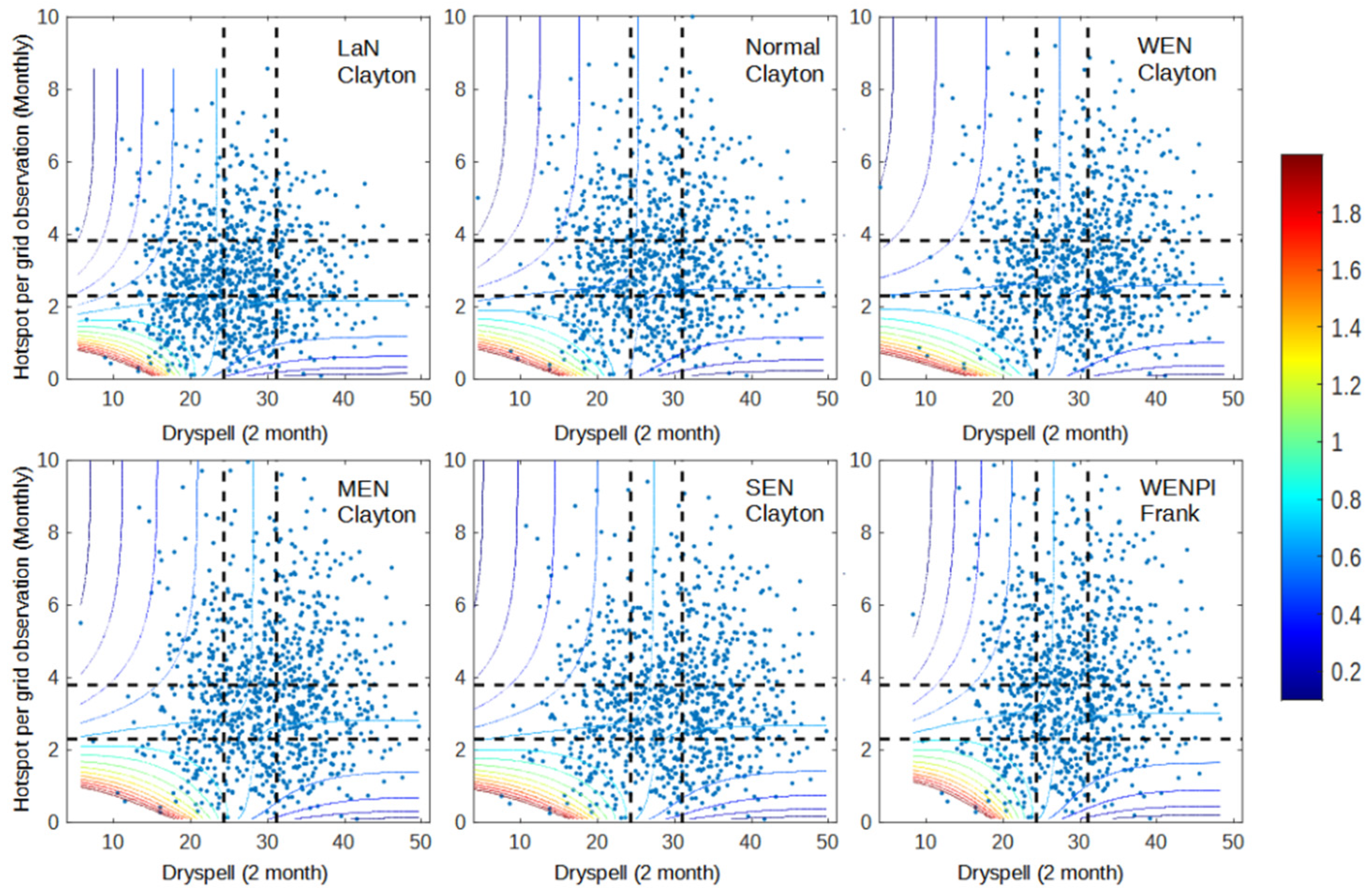
Despite the fact that precipitation anomaly better represents El Niño impact, both dry spell and precipitation anomaly have a close relationship with the hotspot (Figure 3 and Figure 4). Figure 3 and Figure 4 show that the occurrence of El Niño and positive IOD increases the occurrence of data points in the dry condition (top right) and increases the dependency during wet–wet (bottom-left box) and dry–dry conditions (top-right box). However, in terms of modeling, dry spell and hotspot are more likely to be easier to model with copula since all conditions lie within the same copula family, except for SEN, which only occurred in one year. Precipitation anomaly has a more diverse copula family.
From Figure 2, Figure 3 and Figure 4, high dependency (ex: more than 1.6) in dry–dry conditions occurred with any paired variable in all year categories. The difference between each category is in how many data points are in the domain of the dry–dry condition and the range of data that have a high dependency. Thus, there is still a possibility that many hotspots appear in southern Sumatra caused by other local/global phenomena that decrease precipitation during the dry season regardless of ENSO and IOD conditions. This result is as expected because of the fact that there are still many climate factors that can lead to extreme precipitation in southern Sumatra or even non-climate factors that can’t be explained in this research. The main focus for this anomaly is that the data range of dry spells across all year categories is barely different from LaN up to WEN, which occurs more often than MEN, SEN, and WENPI. The main concern about MEN, SEN, and WENPI impact in southern Sumatra is the expansion and prolongation of the drought season that intensifies the land and forest fires that occur every year.

3.1.2. Conditional Survival Probability

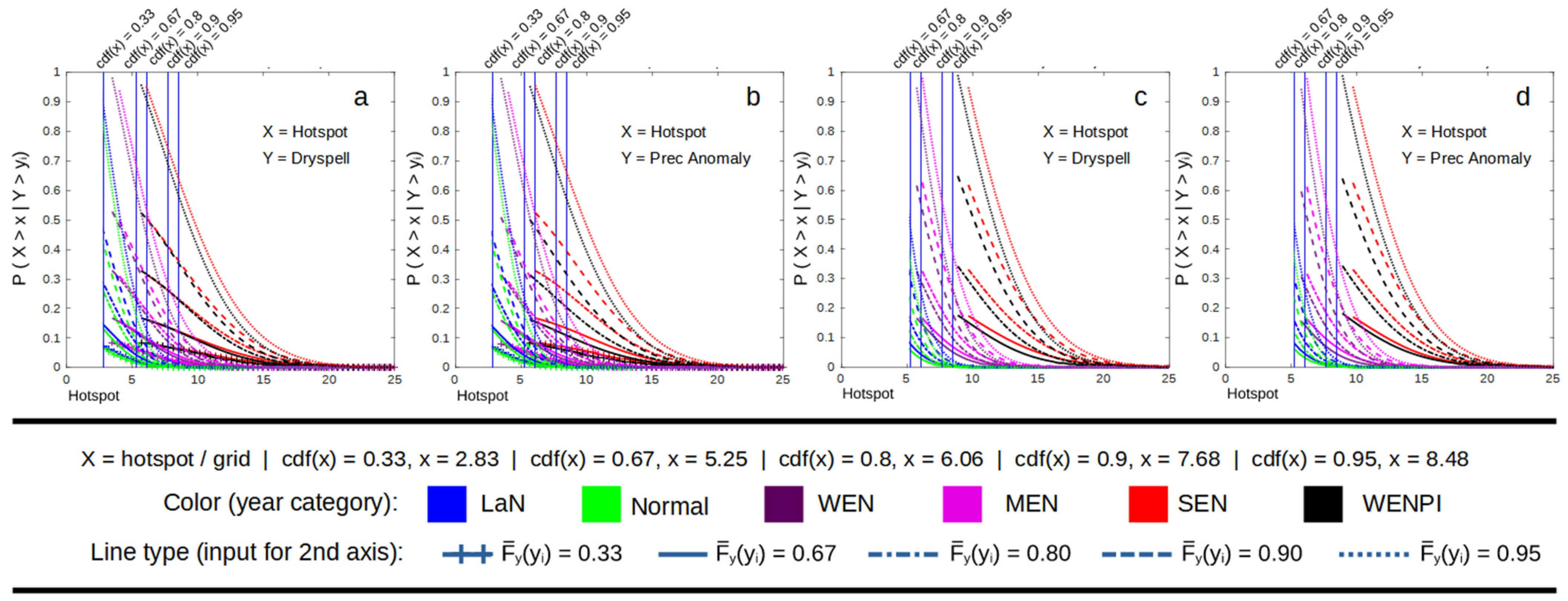
From the dependency analysis, we can conclude that the difference between La Niña, a normal year, and a weak El Niño is insignificant, except in extreme dry conditions (Figure 2, Figure 3 and Figure 4). The difference is more noticeable during MEN, SEN, and WENPI, which can be categorized as extreme conditions. Therefore, in the conditional survival probability analysis, we add another three conditions to the hotspot, which are conditions with 0.8, 0.9, and 0.95 values of the cumulative density function (CDF) to evaluate how El Niño and IOD influence the probability of extreme conditions. This section also only focuses on the probability of hotspots, so dry spells and precipitation anomalies are not analyzed. The result of the conditional survival probability calculation using Equation (9) is a 3D space respective to the values of x and y. It would be difficult to compare multiple graphs from different categories caused by the intersection of the 3D space. Therefore, we add some constant values that represent the wet and dry conditions of common climate analysis to reduce the figure dimension to 2D and make it easier to interpret. For example, during wet conditions of a dry spell (Figure 5a), the graph is calculated using the following equation:
( X > x   | Y > y ) = ( X > x , Y > y ) ( Y > y ) = C * ( F ¯ X ( x ) , F ¯ Y ( y ) ) 1 F ¯ Y ( y ) , F ¯ Y ( y ) = { 0.33 , 0.67 , 0.8 , 0.9 , 0.95 }
Meanwhile, during dry conditions of a dry spell (Figure 5c), the equation is
( X > x   | Y > y ) = ( X > x , Y > y ) ( Y > y ) = C * ( F ¯ X ( x ) , F ¯ Y ( y ) ) 1 F ¯ Y ( y ) , F ¯ Y ( y ) = { 0.67 , 0.8 , 0.9 , 0.95 }
Figure 5 shows that the occurrence of stronger El Niño and positive IOD have a tendency to increase the probability of hotspots by shifting the graph to the right. For example, during a dry spell, the probability of the occurrence of a hotspot with a probability value of occurrence of 0.18 is 2.83 (LaN and Normal), 3.5 (WEN and MEN), and 6.02 (SEN and WENPI). The worst condition (hotspot probability = 1) for each category is 2.6 (LaN and normal), 3.12 (WEN and MEN), and 6 (SEN and WENPI). The increases in probability are not linear. Starting from a weak El Niño, the increases are even higher when reaching a strong El Niño. The survival probability graph of La Niña is similar to a normal year, while the weak El Niño graph is similar to a moderate El Niño. However, if a weak El Niño occurs simultaneously with a positive IOD, the graph will change so that it is close to that of the strong El Niño. This result is interesting, considering that Figure 2 shows that climate conditions (dry spell and prec. anomaly) change quite significantly during a moderate El Niño. These results show that even though a moderate El Niño can increase overall dry conditions significantly compared to a weak El Niño, the change occurs because of the disappearance of data points in wet–wet conditions. Therefore, it is not significantly affecting the probability of hotspot occurrence compared to a weak El Niño condition.

3.1.3. Tail Distribution

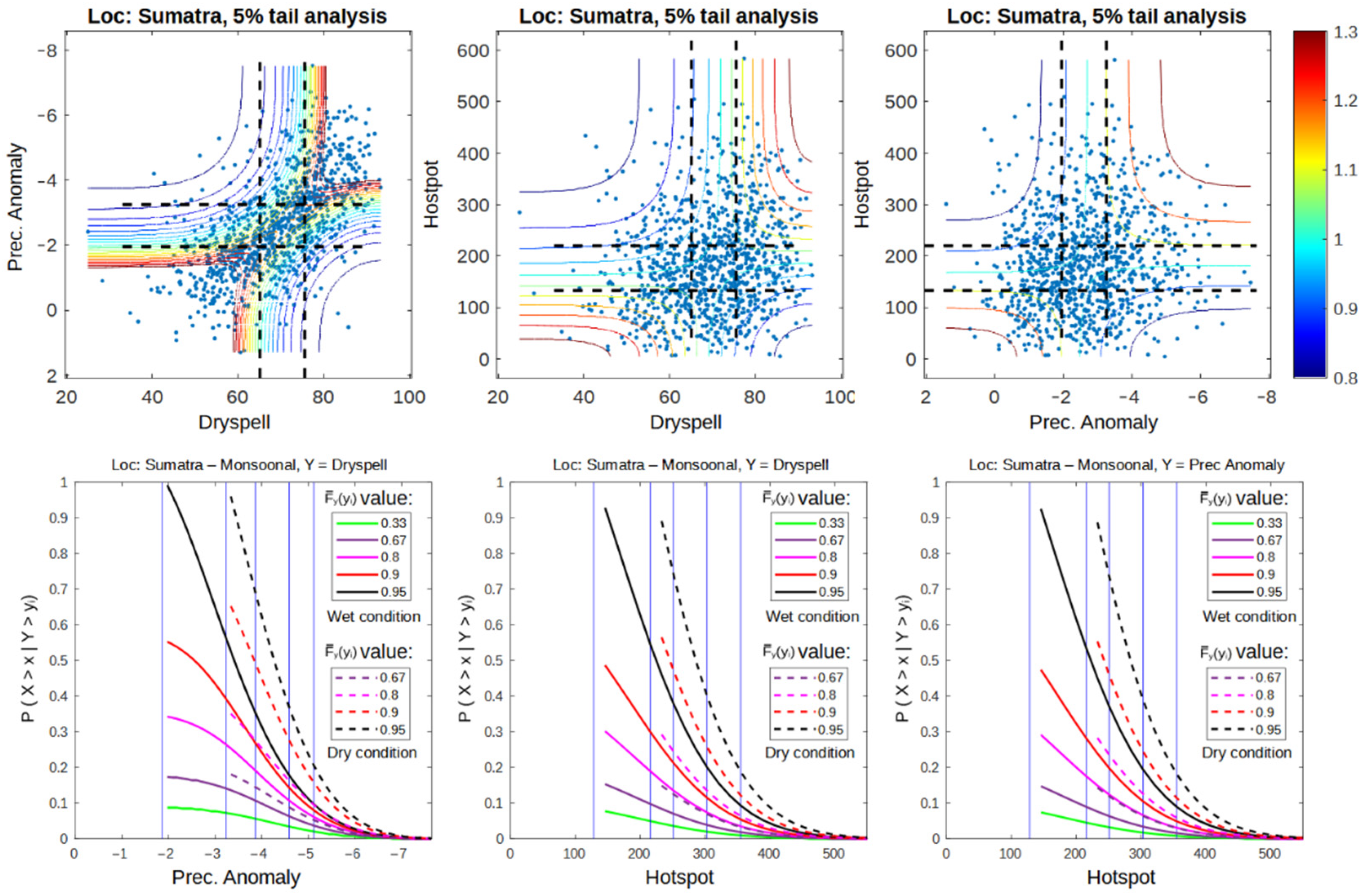
In this section, only 5% of the upper tail of each univariate distribution is examined. This analysis is done to calculate the extreme events regardless of the conditions of ENSO and IOD. Using this analysis, we assume that the hotspot is only triggered by the climate condition of its climate as long as the climate condition meets the 5% upper tail quadrant [37]. The results show that the dependency of dry spell and precipitation anomaly is more consistent in the 5% upper quadrant during wet–wet, normal–normal, and dry–dry conditions. By acknowledge the result in Section 3.1.1 that the dependency between dry spell and precipitation has increased as a result of the increased dry conditions. Therefore, the use of both variables in extreme event modeling can be unnecessary to some degree. This is represented by Figure 6, where dry spell and anomaly result in almost identical dependency (Copula Frank family) when paired with a hotspot, as well as conditional probability graphs when used to calculate the survival probability function of a hotspot.

3.2. Sumatra with Equatorial-Type Precipitation

Equatorial-type precipitation is a precipitation type that occurs in Sumatra with two pairs of rain–dry seasons in one year [6]. Therefore, there are two dry seasons and two rainy seasons in one year. Consequently, the length of the dry season itself has become shorter. The first dry season occurs around January–February, while the second one occurs around June–August. Considering that El Niño and positive IOD impacts on the dry season occur around July–October, the first dry season is not affected by ENSO and IOD [10]. Therefore, the analysis of ENSO and IOD impacts is focused on the second dry season. The year categories in this section follow the previous analysis.

3.2.1. Dependency between Pair of Two Variables

Different from the analysis in previous section, the general association of each variable pair in Sumatra with equatorial-type precipitation is worse than in Section 3.1. The only consistent value of association is only appeared between dry spell and precipitation anomaly, where the associations between both of them and hotspot are close to 0 and have inconsistent direction (positive and negative association) (Table 3). This result is achieved as an impact of the lack of land and forest fire data in the analyzed location from 2001 to 2020. Even though the most consistent result is obtained for dry spell–prec. anomaly, the general dependency is relatively low compared to Section 3.1 analysis, with up to double the dependency during WENPI.
Similar with the general properties, the dependency of each range of data shown by Figure 7, Figure 8 and Figure 9 is relatively very low compared to previous analysis, especially between dry spell and hotspot as well as precipitation anomaly and hotspot. The reason that can be used to justify this result is that there are only a few fire events during the second dry season, so it can be considered an extreme value. As a result, the univariate distribution and obtained copula cannot account for the relationship between climate indicator and hotspot. Even when there was a dry spell and a precipitation anomaly, the high dependency occurred only in wet–wet conditions, with some exceptions in WEN and MEN. This result shows that the conditions during the dry season vary from time to time and make it difficult to model. The lower dependency between the climate indicator and the hotspot makes conditional survival probability analysis unnecessary and inaccurate, so the analysis will be continued straight to the tail analysis.
In general, the higher end (dry–dry condition) of the copula in Figure 7, Figure 8 and Figure 9 has a low dependency (less than 0.4) which is much lower compared to the lower end (wet–wet condition). Even though on dry spell–prec. anomaly analysis, the higher-end dependency is still relatively low compared to the previous section’s analysis. This result represents that precipitation conditions in the second dry season of northern Sumatra are more diverse than in the southern dry season. Thus, there are other factors that influenced dry spells and prec. anomalies independently as well as over a shorter duration, which can’t be explained in this result. For example, the average daily precipitation for the last 2 months is less than average but still greater than 1 mm. Thus, it is counted as dry conditions in terms of prec. anomaly but categorized as wet conditions for the dry spell condition, and vice versa. Therefore, the average drought condition is not as severe, which can lead to high dependency with hotspot occurrence. In other words, land and forest fires that happen in northern Sumatra during the second dry season are more likely caused by very rare climate anomalies, such as what happened in 2013 [42], or other factors regardless of the climate condition, such as deforestation.

3.2.2. Tail Distribution

As mentioned before, there have been only a few large fire events during the second dry season on Sumatra with equatorial-type precipitation. One of the most significant events occurred in 2013 [42], with a total rainfall of 56.08 mm during the peak fire events in June. Considering that 2013 was a normal year, the analysis would be even more inaccurate if we had not separated the extreme event from the previous analysis.
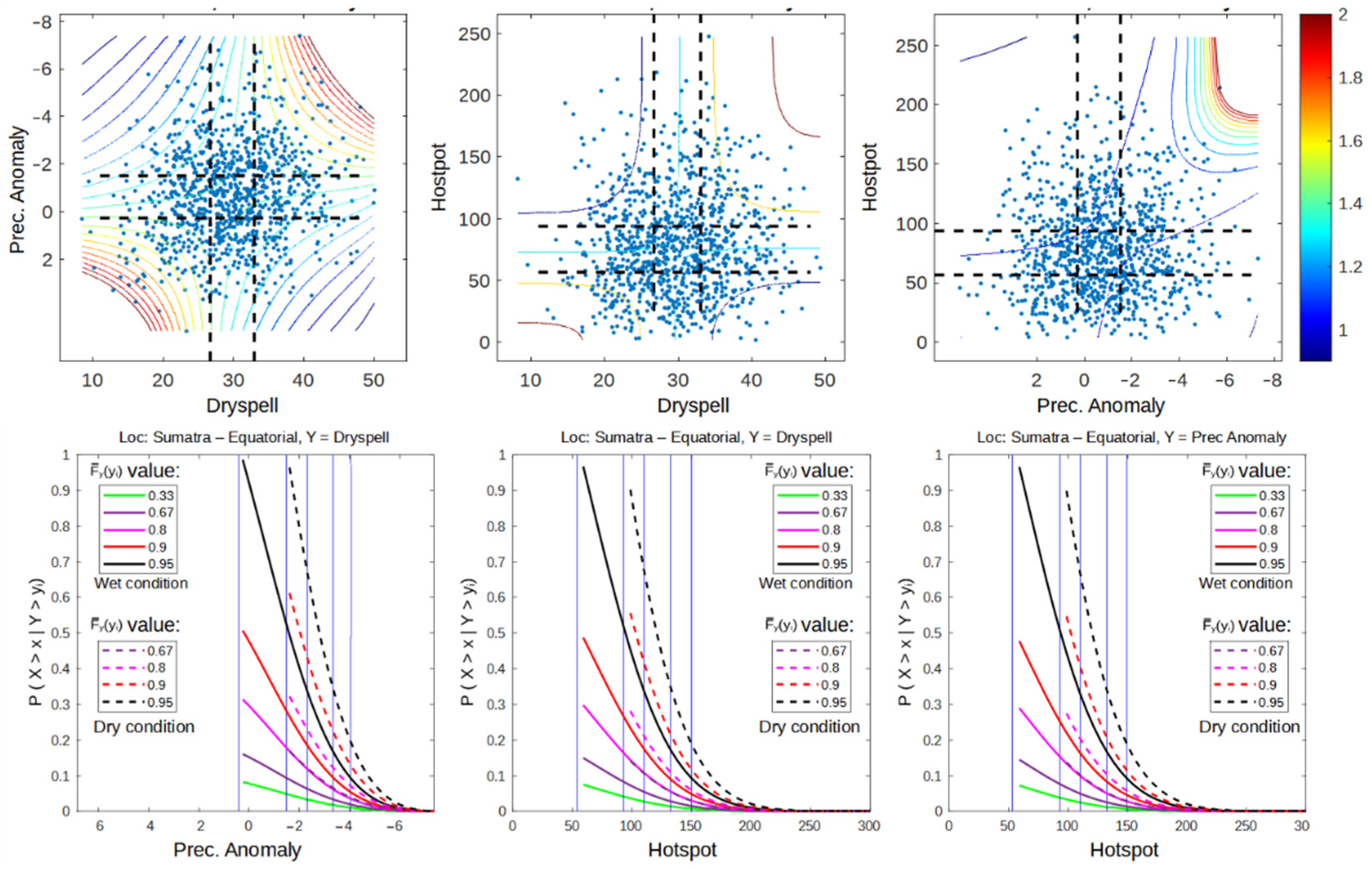
Figure 10 shows that during extreme events, the dependence in all variable pairs’ increases significantly, particularly in the dry condition. Dry spells and prec. anomalies have more consistent dependency following the Gaussian copula family during extreme events. Therefore, dependency in wet–wet conditions is quite similar to dependency in dry–dry conditions. Significant improvement was also observed in the dry condition of dry spell–hotspot and prec. anomaly–hotspot dependency, implying that more fire events occurred in dry–dry conditions when compared to the previous section. However, all pairs of variables lie in different copula families, which are Gaussian (dry spell–prec. anomaly), Frank (dry spell–hotspot), and Gumbel (prec. anomaly–hotspot). This result shows that all three variables have different characteristics from each other and can be difficult to model.

3.2.3. Madden–Julian Oscillation Impact on the First DRY Season

The Madden–Julian Oscillation (MJO) is the major intra-seasonal (30–60-day) variability in the tropics, characterized by the eastward propagation of cloud clusters and precipitation from the Indian Ocean to the western Pacific Ocean [13]. There are eight phases of MJO, which can be measured using the RMM1 and RMM2 indexes [16], each with different impacts than others, namely:
  • Phase 1 (RMM1 < 0, RMM2 < 0, RMM1 > RMM2): enhanced convection (rainfall) develops over the western Indian Ocean.
  • Phases 2 (RMM1 < 0, RMM2 < 0, RMM1 < RMM2) and 3 (RMM1 > 0, RMM2 < 0, RMM1 < |RMM2|): enhanced convection (rainfall) moves slowly eastward over Africa, the Indian Ocean, and parts of the Indian subcontinent.
  • Phase 4 (RMM1 > 0, RMM2 < 0, RMM1 > |RMM2|) and 5 (RMM1 > 0, RMM2 > 0, RMM1 > RMM2): enhanced convection (rainfall) has reached the maritime continent (Indonesia and the West Pacific).
  • Phase 6 (RMM1 > 0, RMM2 > 0, RMM1 < RMM2), 7 (RMM1 < 0, RMM2 > 0, |RMM1| < RMM2) and 8 (RMM1 < 0, RMM2 > 0, |RMM1| > RMM2): enhanced rainfall moves further eastward over the western Pacific, eventually dying out in the central Pacific.
Many researchers have explained and demonstrated how the MJO affects extreme precipitation in Indonesia [18,19,43]. The strongest impact of the MJO occurred in the western part of Indonesia, which is around Sumatra, which has an equatorial precipitation type [18]. The MJO reduced precipitation in those areas in Indonesia during phases 5, 6, 7, and 8. Though the MJO impacted from western to eastern Indonesia, the impact was often negated by other local—though of a wider atmospheric scale—phenomena that have more significant influence over those areas, such as monsoon winds [17]. Therefore, analysis in this section is only focused on the period around the first dry season (January–March). The influence of phases 5–8 will be analyzed by comparing each phase with the data from phase 1–4.
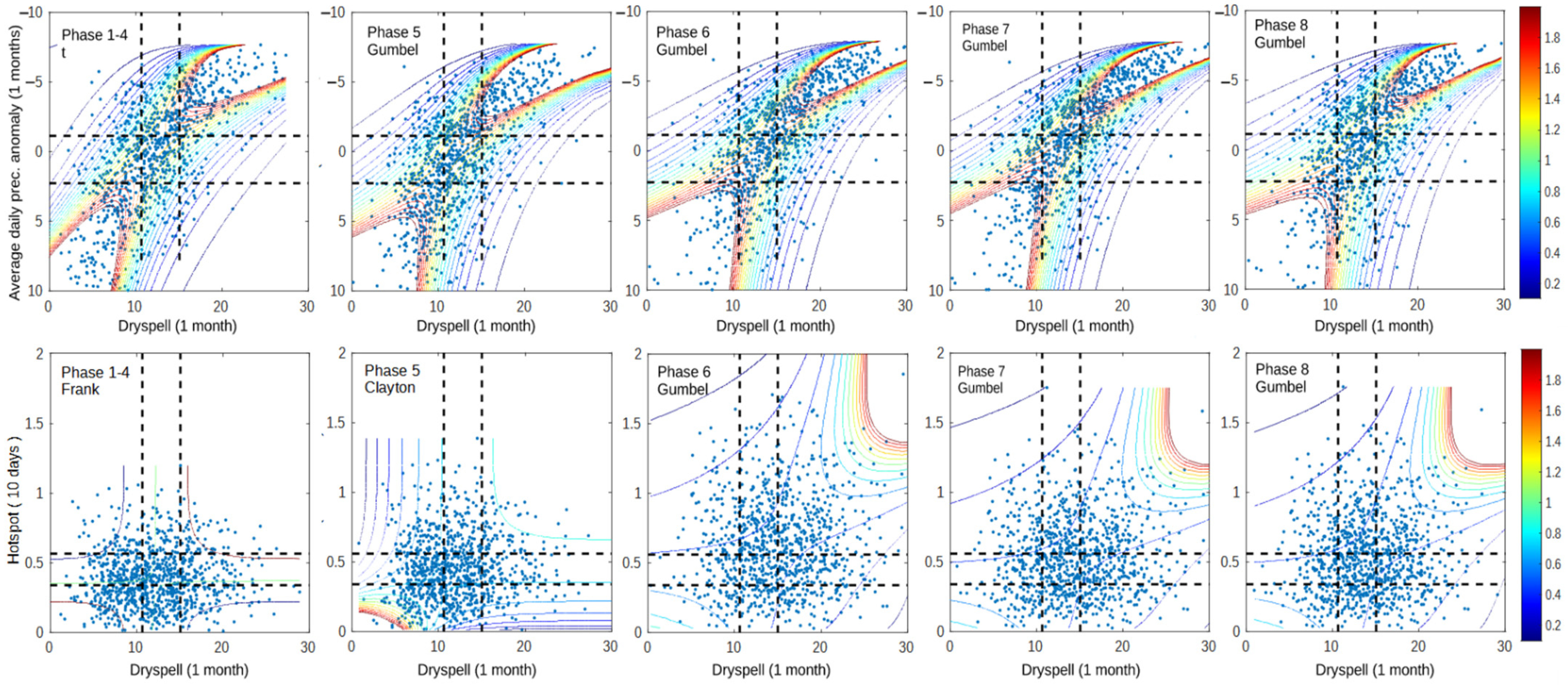
Figure 11 shows that phases 6, 7, and 8 of the MJO have a significant impact on the result. Even though the difference in dry spell–prec. anomaly dependency is not clear, the difference in the dependency of dry spell–hotspot has increased significantly compared to phases 1–4 and 5. Even though the general property of phase 5 is higher for dry spell–prec. anomaly than phase 8, as shown by Table 4, the higher dependency is more related to the wet condition during phase 5. This is also represented by higher dependency in the wet-condition phase 5 graph of dry spell–hotspot. The small difference in dry spell–prec. anomaly is likely caused by the inconsistency of the prec. anomaly variable’s behavior. This result is consistent with previous research, which found that precipitation around Riau is reduced during MJO phases compared to normal conditions [44,45,46]. Figure 12 depicts the comparison of the impacts for each phase.
Figure 11 shows that dry spells and prec. anomalies in the 1st dry season of northern Sumatra are very related to each other from the wet–wet condition to the dry–dry condition. This result represents that both of them can be used alternately to represent the severity of the dry season for all conditions. In the dry–dry condition, phases 6–8 of the MJO can increase the dry spell–prec. anomaly relation by narrowing the top-right shape of the copula distribution. Moreover, phases 6–8 of the MJO can increase the dependency of dry spells and hotspots significantly compared to other phases. Even though the number of dependency data points greater than 1 is very few, the number of data points with more than 1 hotspot in phases 6–8 is much higher than in phases 1–5. This result shows the importance of the MJO in influencing drought conditions in the 1st dry season of northern Sumatra. Although the duration of the dry season itself is very short (1–2 months), MJO extremes that occurred during other climate anomalies can lead to much more severe dry seasons, such as what happened in 2014 [15], which caused more than 6000 hotspots to occur in 1 month [13].
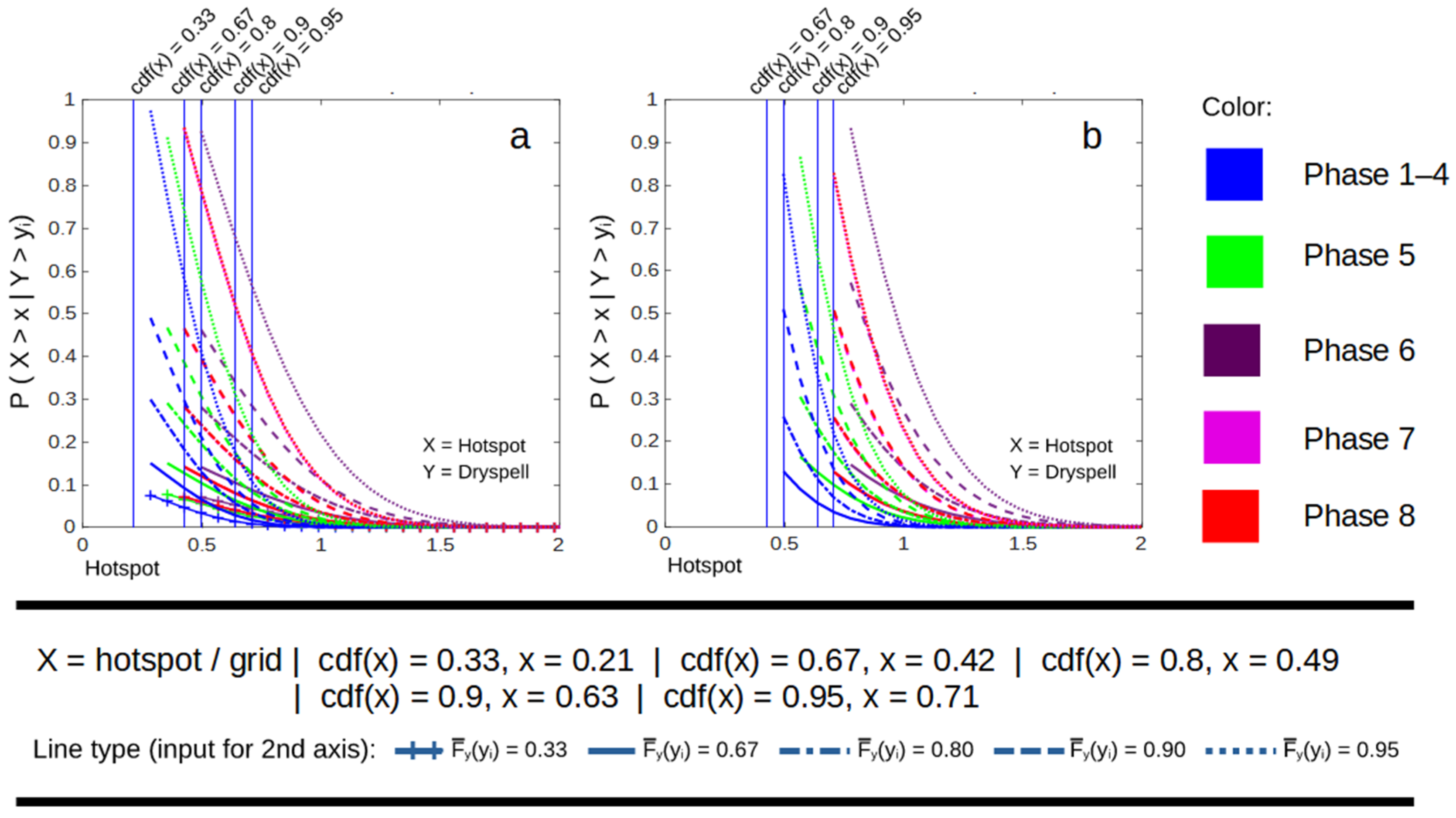
In increasing hotspot probabilities, phase 6 has the highest impact on dry spell–hotspot joint probability, followed by phases 8 and 7, which have very similar impacts. An unclear impact occurred in phase 5, resulting in less dependency in Figure 11. The probability of a hotspot in Figure 12 is increased compared to phases 1–4. Figure 12 depicts the dryer conditions during phase 5, which is more consistent with previous research [47,48,49].
Despite having higher dependency when a certain MJO phase occurred, the tail analysis of the 5% upper quadrant from dry spell–prec. anomaly and dry spell–hotspot resulted in satisfying results. In the 5% upper quadrant, the dependency between dry spell and precipitation anomaly is much higher in wet–wet, normal–normal, and dry–dry conditions (Figure 13). Although not as high as dry spell–prec. anomaly, the dependency of dry spell–hotspot is higher and more consistent in wet–wet, normal–normal, and dry–dry conditions. This result represents that the used variables are more predictable during extreme events.

4. Discussion

Results of this research are mostly in line with previous research, where El Niño and positive IOD have contributed to increased dry season conditions as well as hotspot occurrences [7,8,13]. The contribution of this research regarding El Niño and the positive IOD impact on South Sumatra is to show that the impact is not linear [14,50,51]. The result can be separated from observed data by looking at how significant the difference between each category is compared to a normal year or how close the dependency of paired variables is to each category. This finding is important for future research in similar areas to give alternate solutions in order to increase the number of observed data by categorizing weak and moderate El Niño as one category (probability of 2.6 hotspots occurring per grid is 1), as well as strong El Niño and positive IOD during weak El Niño as one category of extreme events (probability of 6 hotspots occurring per grid is 1). Furthermore, this finding acknowledges the importance of the ENSO-IOD teleconnection impact [52,53] on southern Sumatra.
Even during a weak El Niño, the occurrence of a positive IOD can lead to much more severe conditions ( ρ [ dryspell , hotspot ] = 0.183 ) than a strong El Niño condition ( ρ [ dryspell , hotspot ] = 0.179 ) [54,55], especially when a weak El Niño is considered a more common event and does not really affect dry season conditions in southern Sumatra. Therefore, more in-depth research about how it influences land and forest fires needs to be done to get more information that can be used to predict future fire events. Section 3.2.1 shows that El Niño and positive IOD didn’t have a clear impact on either the dry season (indicated by dry spell and precipitation anomaly) or the hotspot occurrence in South Sumatra with equatorial-type precipitation. Even though the second dry season occurs around June–September, the dry season is over when the peak impact of El Niño and positive IOD occurs (usually around August–October) [56,57].
The results in Section 3.2.3 show that the Madden–Julian oscillation has quite a significant impact on the dependency of a high number of dryspell–hotspots in northern Sumatra. The probability of 1 hotspot occurring is increased from 0 (phase 1–4) to a maximum of around 0.2 (phase 6) during wet conditions. Even more, the probability is double (around 0.4 in phase 6) if known to be in dry conditions. Even though the impact of dry spell–prec. anomaly dependency is not clear (only noticeable in wet–wet conditions), this finding is important for the development process of hotspot prediction models in the future. However, the finding about the MJO’s impact on forest fires can be improved by developing a new index that represents the downward location and amplitude of the MJO phase. The current RMM1 and RMM2 indexes used in this research represent the location and amplitude of the upward MJO, which is more related to the increasing precipitation in the surrounding area. Otherwise, the downward MJO effect is to decrease precipitation in the surrounding area, which leads to more dry conditions. Lastly, this research also shows that the use of dry spells and precipitations is tricky in hotspot analysis. Prec. anomaly has a better response to dryer conditions affected by ENSO and IOD, while it completely fails to result in dependency with hotspots in Section 3.2.3. However, both variables have similar behavior during extreme conditions since the dry spell–prec. anomaly has a much higher dependency on the 5% upper quadrant of observed data.
From the tail distribution analysis, we can state that during extreme condition, dry spells and precipitation anomalies have high dependency (more than 1.6) across all of the data range. Meanwhile, the dependency of dry spell–hotspot as well as prec. anomaly-hotspot is also high (more than 1.1 from a max of 1.2 in monsoonal, 1.6 from 1.8 in equatorial in 1st dry season) for the wet–wet and dry–dry conditions of the graph. Obviously, the wet–wet condition is obtained from areas that have more precipitation during dry seasons and fewer hotspots which can be ignored during dry season analysis. The general association between dry spells and hotspots in southern Sumatra in a monsoonal dry season is 0.18, which is close to the WENPI category. Meanwhile, the general association between dry spells and hotspots in the 1st dry season of northern Sumatra is 0.27, which is higher than all values in Table 4. In this case, the higher general association value is caused by the increased number of hotspot observations followed by the increases in dry conditions. This result shows that the analyzed variables, especially dry spells and hotspots, are much easier to predict during extreme conditions compared to non-extreme conditions regardless of the cause of the extreme dry season.
This research assumes that land and forest fires in Sumatra are not affected by non-climate variables, such as land type and condition, human behavior, political and industrial policy, etc. Obviously, the result will become more accurate when acknowledging those variables. However, those variables are often difficult to measure, may vary from time to time, and are difficult to predict, especially those related to human behavior. On the other hand, using only climate conditions shows the land and forest fire conditions if there is no significant effort from residents and government to reduce the scale and duration of land and forest fire events. Research in this field is important for increasing the awareness of the government of anticipating future events when extreme dry conditions happen.

Author Contributions

Conceptualization, S.N. and A.S.; methodology, A.S. and P.S.; software, P.S.; validation, S.N., A.S. and P.S.; formal analysis, S.N.; investigation, A.S.; resources, S.N. and A.S.; data curation, P.S.; writing—original draft preparation, P.S.; writing—review and editing, S.N.; visualization, P.S.; supervision, S.N. and A.S.; project administration S.N. All authors have read and agreed to the published version of the manuscript.

Funding

This research received no external funding.

Institutional Review Board Statement

Not applicable.

Informed Consent Statement

Not applicable.

Data Availability Statement

Not applicable.

Acknowledgments

Acknowledgment is given to the Meteorology, Climatology, and Geophysical Agency of Indonesia for the invaluable assistance, as well as the Department of Mathematics at IPB University for the strong support.

Conflicts of Interest

The authors declare no conflict of interest.

References

  1. Diffenbaugh, N.S.; Singh, D.; Mankin, J.S.; Horton, D.E.; Swain, D.L.; Touma, D.; Charland, A.; Liu, Y.; Haugen, M.; Tsiang, M.; et al. Quantifying the influence of global warming on unprecedented extreme climate events. Proc. Natl. Acad. Sci. USA 2017, 114, 4881–4886. [Google Scholar] [CrossRef] [PubMed] [Green Version]
  2. Seneviratne, S.I.; Nicholls, N.; Easterling, D.; Goodess, C.M.; Kanae, S.; Kossin, J.; Luo, Y.; Marengo, J.; McInnes, K.; Rahimi, M.; et al. Changes in climate extremes and their impacts on the natural physical environment. In Managing the Risks of Extreme Events and Disasters to Advance Climate Change Adaptation; Field, C.B., Barros, V., Stocker, T.F., Qin, D., Dokken, D.J., Ebi, K.L., Mastrandrea, M.D., Mach, K.J., Plattner, S.K., Allen, G.-K., et al., Eds.; A Special Report of Working Groups I and II of the Intergovernmental Panel on Climate Change (IPCC); Cambridge University Press: Cambridge, UK; New York, NY, USA, 2012; pp. 109–230. [Google Scholar]
  3. Tabari, H. Climate change impact on flood and extreme precipitation increases with water availability. Sci. Rep. 2020, 10, 1–10. [Google Scholar] [CrossRef] [PubMed]
  4. Cai, W.; Santoso, A.; Collins, M.; Dewitte, B.; Karamperidou, C.; Kug, J.S.; Lengaigne, M.; McPhaden, M.J.; Stuecker, M.F.; Taschetto, A.S.; et al. Changing El Niño–Southern Oscillation in a warming climate. Nat. Rev. Earth Environ. 2021, 2, 628. [Google Scholar] [CrossRef]
  5. Yulianti, N.; Hayasaka, H.; Sepriando, A. Recent Trends of Fire Occurrence in Sumatra (Analysis Using MODIS Hotspot Data): A Comparison with Fire Occurrence in Kalimantan. Open J. For. 2013, 3, 129–137. [Google Scholar] [CrossRef] [Green Version]
  6. Septiawan, P.; Nurdiati, S.; Sopaheluwakan, A. Analisis Empirical Orthogonal Function (Eof) dan Transformasi Fourier pada Sinyal Curah Hujan Indonesia. In Proceeding of the Seminar Nasional Pendidikan Matematika, Yogyakarta, Indonesia, 11 November 2017. [Google Scholar]
  7. Septiawan, P.; Nurdiati, S.; Sopaheluwakan, A. Numerical Analysis using Empirical Orthogonal Function Based on Multivariate Singular Value Decomposition on Indonesian Forest Fire Signal. IOP Conf. Ser. Earth Environ. Sci. 2019, 303, 012053. [Google Scholar] [CrossRef]
  8. Nurdiati, S.; Sopaheluwakan, A.; Agustina, A.; Septiawan, P. Multivariate analysis on Indonesian forest fire using combined em-pirical orthogonal function and covariance matrices. In IOP Conference Series: Earth and Environmental Science; IOP Publishing: Bristol, UK, 2019; p. 12048. [Google Scholar]
  9. Nur’utami, M.N.; Hidayat, R. Influences of IOD and ENSO to Indonesian Rainfall Variability: Role of Atmosphere-ocean Inter-action in the Indo-pacific Sector. Procedia Environ. Sci. 2016, 33, 196–203. [Google Scholar] [CrossRef] [Green Version]
  10. Trenberth, K.E. The Definition of El Niño. Bull. Am. Meteorol. Soc. 1997, 78, 2771–2778. [Google Scholar] [CrossRef] [Green Version]
  11. Saji, N.H.; Goswami, B.N.; Vinayachandran, P.N.; Yamagata, T. A dipole mode in the tropical Indian Ocean. Nature 1999, 401, 360–363. [Google Scholar] [CrossRef]
  12. Dafri, M.; Nurdiati, S.; Sopaheluwakan, A. Quantifying ENSO and IOD impact to titik api in Indonesia based on Heterogeneous Correlation Map (HCM). J. Phys. Conf. Ser. 2021, 1896, 012150. [Google Scholar] [CrossRef]
  13. Nurdiati, S.; Sopaheluwakan, A.; Septiawan, P. Spatial and Temporal Analysis of El Niño Impact on Land and Forest Fire in Kalimantan and Sumatra. Agromet 2021, 35, 1–10. [Google Scholar] [CrossRef]
  14. Nurdiati, S.; Sopaheluwakan, A.; Julianto, M.T.; Septiawan, P.; Rohimahastuti, F. Modelling and analysis impact of El Nino and IOD to land and forest fire using polynomial and generalized logistic function: Cases study in South Sumatra and Kalimantan, Indonesia. Model. Earth Syst. Environ. 2021, 1–16. [Google Scholar] [CrossRef]
  15. McBride, J.L.; Sahany, S.; Hassim, M.E.; Nguyen, C.M.; Lim, S.-Y.; Rahmat, R.; Cheong, W.-K. The 2014 record dry spell at Singapore: An intertropical convergence zone (itcz) drought. Bull. Am. Meteorol. Soc. 2015, 96, S126–S130. [Google Scholar] [CrossRef]
  16. Madden, R.A.; Julian, P.R. Description of global-scale circulation cells in the tropics with a 40–50 days period. J. Atmos. Sci. 1972, 29, 1109–1123. [Google Scholar] [CrossRef]
  17. Pramuwardani, I.; Hartono, S.; Sopaheluwakan, A. The inCuence of Madden–Julian Oscillation on local-scale phenomena over Indonesia during the Western northPaciBc and Australian Monsoon phases. Forum Geogr. 2018, B31, 156–169. [Google Scholar] [CrossRef] [Green Version]
  18. Fadhlil, R.M.; Sandro, L.; Sonni, S. Impacts of the Madden Julian Oscillation on Precipitation Extremes in Indonesia. Int. J. Clim. 2021, 41, 1970–1984. [Google Scholar]
  19. Wijayanti, A.V.; Hidayat, R.; Faqih, A.; Alfahmi, F. The Impact of the Interaction between Madden-Julian Oscillation and Cold Surge, on Rainfall over Western Indonesia. Indones. J. Geogr. 2021, 53, 245–253. [Google Scholar] [CrossRef]
  20. Xie, P.; Joyce, R.; Wu, S.; Yoo, S.-H.; Yarosh, Y.; Sun, F.; Lin, R. NOAA CDR Program. NOAA Climate Data Record (CDR) of CPC Morphing Technique (CMORPH) High Resolution Global Precipitation Estimates, Version 1 [Indicate Subset]; NOAA National Centers for Environmental Information: Silver Spring, MD, USA, 2019. [Google Scholar] [CrossRef]
  21. An, Y.; Zhao, W.; Li, C.; Liu, Y. Evaluation of Six Satellite and Reanalysis Precipitation Products Using Gauge Observations over the Yellow River Basin, China. Atmosphere 2020, 11, 1223. [Google Scholar] [CrossRef]
  22. MODIS Collection 61 NRT Hotspot/Active Fire Detections MCD14DL Distributed from NASA FIRMS. Available online: https://earthdata.nasa.gov/firms (accessed on 21 March 2022).
  23. Francisco de Castro. Fitmethis 2022; MATLAB Central File Ex-Change. Available online: https://www.mathworks.com/matlabcentral/fileexchange/40167-fitmethis (accessed on 15 February 2022).
  24. Cousineau, D.; Brown, S.; Heathcote, A. Fitting distributions using maximum likelihood: Methods and packages. Behav. Res. Methods Instrum. Comput. 2004, 36, 742–756. [Google Scholar] [CrossRef] [PubMed]
  25. Wang, X. Random signal processing and spectrum analysis in vehicle noise and vibration refinement. In Vehicle Noise and Vibration Refinement; Woodhead Publishing: Sawston, UK, 2010; pp. 93–116. [Google Scholar] [CrossRef]
  26. Bali, T.G. The generalized extreme value distribution. Econ. Lett. 2003, 79, 423–427. [Google Scholar] [CrossRef]
  27. Mscavnicky. Copula Matlab Master. Github Repository. 2019. Available online: https://github.com/mscavnicky/copula-matlab (accessed on 15 February 2022).
  28. Grothe, O.; Schnieders, J.; Segers, J. Measuring association and dependence between random vectors. J. Multivar. Anal. 2014, 123, 96–110. [Google Scholar] [CrossRef]
  29. Chadjiconstantinidis, S.; Vrontos, S. On a renewal risk process with dependence under a Farlie–Gumbel–Morgenstern copula. Scand. Actuar. J. 2011, 2014, 125–158. [Google Scholar] [CrossRef] [Green Version]
  30. Zhang, L.; Singh, V.P. Symmetric archimedean copulas. In Copulas and Their Applications in Water Resources Engineering; Zhang, L., Singh, V.P., Eds.; Cambridge University Press: Cambridge, UK, 2019; pp. 123–171. [Google Scholar]
  31. Aldhufairi, F.A.-A.; Samanthi, R.G.; Sepanski, J.H. New Families of Bivariate Copulas via Unit Lomax Distortion. Risks 2020, 8, 106. [Google Scholar] [CrossRef]
  32. Hasebe, T. Copula-based maximum-likelihood estimation of sample-selection models. Copula-based maximum-likelihood es-timation of sample-selection models. Stata J. 2013, 13, 547–573. [Google Scholar] [CrossRef] [Green Version]
  33. Akaike, H. Likelihood of a model and information criteria. J. Econ. 1981, 16, 3–14. [Google Scholar] [CrossRef]
  34. Charpentier, A. Tail distribution and dependence measures. In Proceedings of the 34th ASTIN Conference, Berlin, Germany, 24 August 2003; pp. 1–25. [Google Scholar]
  35. Juri, A.; Wüthrich, M.V. Copula convergence theorems for tail events. Insur. Math. Econ. 2002, 30, 405–420. [Google Scholar] [CrossRef]
  36. Oakes, D. On the preservation of copula structure under truncation. Can. J. Stat. Rev. Can. Stat. 2005, 33, 465–468. [Google Scholar] [CrossRef]
  37. Davidow, M.; Matteson, D.S. Copula Quadrant Similarity for Anomaly Scores. arXiv 2021, arXiv:2101.02330v1. [Google Scholar]
  38. Ardiansyah, M.; Boer, R.; Situmorang, A. Typology of land and forest fire on South Sumatra, Indonesia Based on Assessment of MODIS Data. IOP Conf. Ser. Earth Environ. Sci. 2017, 54, 012058. [Google Scholar] [CrossRef]
  39. Yulihastin, E.; Febrianti, N. Trismidianto. In Impacts of El Niño and IOD on the Indonesian Climate; National Institute of Aeronautics and Space (LAPAN): Jakarta, Indonesia, 2009. [Google Scholar]
  40. Avia, L.; Sofiati, I. Analysis of El Niño and IOD Phenomenon 2015/2016 and Their Impact on Rainfall Variability in Indonesia. IOP Conf. Ser. Earth Environ. Sci. 2018, 166, 012034. [Google Scholar] [CrossRef] [Green Version]
  41. Kurniadi, A.; Weller, E.; Min, S.; Seong, M. Independent ENSO and IOD impacts on rainfall extremes over Indonesia. Int. J. Clim. 2021, 41, 3640–3656. [Google Scholar] [CrossRef]
  42. Kusumaningtyas, S.D.A.; Aldrian, E. Impact of the June 2013 Riau province Sumatera smoke haze event on regional air pollution. Environ. Res. Lett. 2016, 11, 075007. [Google Scholar] [CrossRef]
  43. Hidayat, R. Modulation of Indonesian Rainfall Variability by the Madden-julian Oscillation. Procedia Environ. Sci. 2016, 33, 167–177. [Google Scholar] [CrossRef] [Green Version]
  44. Peatman, S.C.; Matthews, A.J.; Stevens, D.P. Propagation of the Madden-Julian Oscillation through the Maritime Continent and scale interaction with the diurnal cycle of precipitation. Q. J. R. Meteorol. Soc. 2013, 140, 814–825. [Google Scholar] [CrossRef]
  45. Zhu, B.; Du, Y.; Gao, Z. Influences of MJO on the Diurnal Variation and Associated Offshore Propagation of Rainfall near Western Coast of Sumatra. Atmosphere 2022, 13, 330. [Google Scholar] [CrossRef]
  46. Haki, M. Precipitation over Indonesia in Observations and Global Reforecasts and Impact of the Madden Julian Oscillation. Master’s Thesis, North Carolina State University, Raleigh, NC, USA.
  47. Rauniyar, S.P.; Walsh, K. Scale Interaction of the Diurnal Cycle of Rainfall over the Maritime Continent and Australia: Influence of the MJO. J. Clim. 2011, 24, 325–348. [Google Scholar] [CrossRef]
  48. Fujita, M.; Yoneyama, K.; Mori, S.; Nasuno, T.; Satoh, M. Diurnal Convection Peaks over the Eastern Indian Ocean off Sumatra during Different MJO Phases. J. Meteorol. Soc. Jpn. Ser. 2011, 89A, 317–330. [Google Scholar] [CrossRef] [Green Version]
  49. Kamimera, H.; Mori, S.; Yamanaka, M.D.; Syamsudin, F. Modulation of Diurnal Rainfall Cycle by the Madden-Julian Oscillation Based on One-Year Continuous Observations with a Meteorological Radar in West Sumatera. SOLA 2012, 8, 111–114. [Google Scholar] [CrossRef] [Green Version]
  50. Pan, X.; Chin, M.; Ichoku, C.M.; Field, R.D. Connecting Indonesian Fires and Drought with the Type of El Niño and Phase of the Indian Ocean Dipole During 1979–2016. J. Geophys. Res. Atmos. 2018, 123, 7974–7988. [Google Scholar] [CrossRef]
  51. Field, R.D.; van der Werf, G.R.; Fanin, T.; Fetzer, E.J.; Fuller, R.; Jethva, H.; Levy, R.; Livesey, N.J.; Luo, M.; Torres, O.; et al. Indonesian fire activity and smoke pollution in 2015 show persistent nonlinear sensitivity to El Niño-induced drought. Proc. Natl. Acad. Sci. USA 2016, 113, 9204–9209. [Google Scholar] [CrossRef] [Green Version]
  52. Cai, W.; Van Rensch, P.; Cowan, T.; Hendon, H.H. Teleconnection Pathways of ENSO and the IOD and the Mechanisms for Impacts on Australian Rainfall. J. Clim. 2011, 24, 3910–3923. [Google Scholar] [CrossRef]
  53. Yuan, D.; Hu, X.; Xu, P.; Zhao, X.; Masumoto, Y.; Han, W. The IOD-ENSO precursory teleconnection over the tropical Indo-Pacific Ocean: Dynamics and long-term trends under global warming. J. Oceanol. Limnol. 2017, 36, 4–19. [Google Scholar] [CrossRef]
  54. Okta, D.L.; Sutriyono, E.; Iskandar, I. Respective Influences of Indian Ocean Dipole and El Niño-Southern Oscillation on Indonesian Precipitation. J. Math. Fund. Sci. 2018, 50, 257–272. [Google Scholar]
  55. Le, T.; Ha, K.-J.; Bae, D.-H.; Kim, S.-H. Causal effects of Indian Ocean Dipole on El Niño–Southern Oscillation during 1950–2014 based on high-resolution models and reanalysis data. Environ. Res. Lett. 2020, 15, 1040b6. [Google Scholar] [CrossRef]
  56. Hong, C.-C.; Lu, M.-M.; Kanamitsu, M. Temporal and spatial characteristics of positive and negative Indian Ocean dipole with and without ENSO. J. Geophys. Res. Earth Surf. 2008, 113, D08107. [Google Scholar] [CrossRef] [Green Version]
  57. Xue, C.; Dong, Q.; Si, F.; Xie, J.; Cunjin, X.; Qing, D.; Fengtai, S.; Jiong, X. Spatio-temporal structure of SST in El Niño regions and its relationships with zonal displacement anomaly of western Pacific warm pool. In Proceedings of the 2011 IEEE International Geoscience and Remote Sensing Symposium, Vancouver, BC, Canada, 24–29 July 2011; pp. 2025–2028. [Google Scholar] [CrossRef]
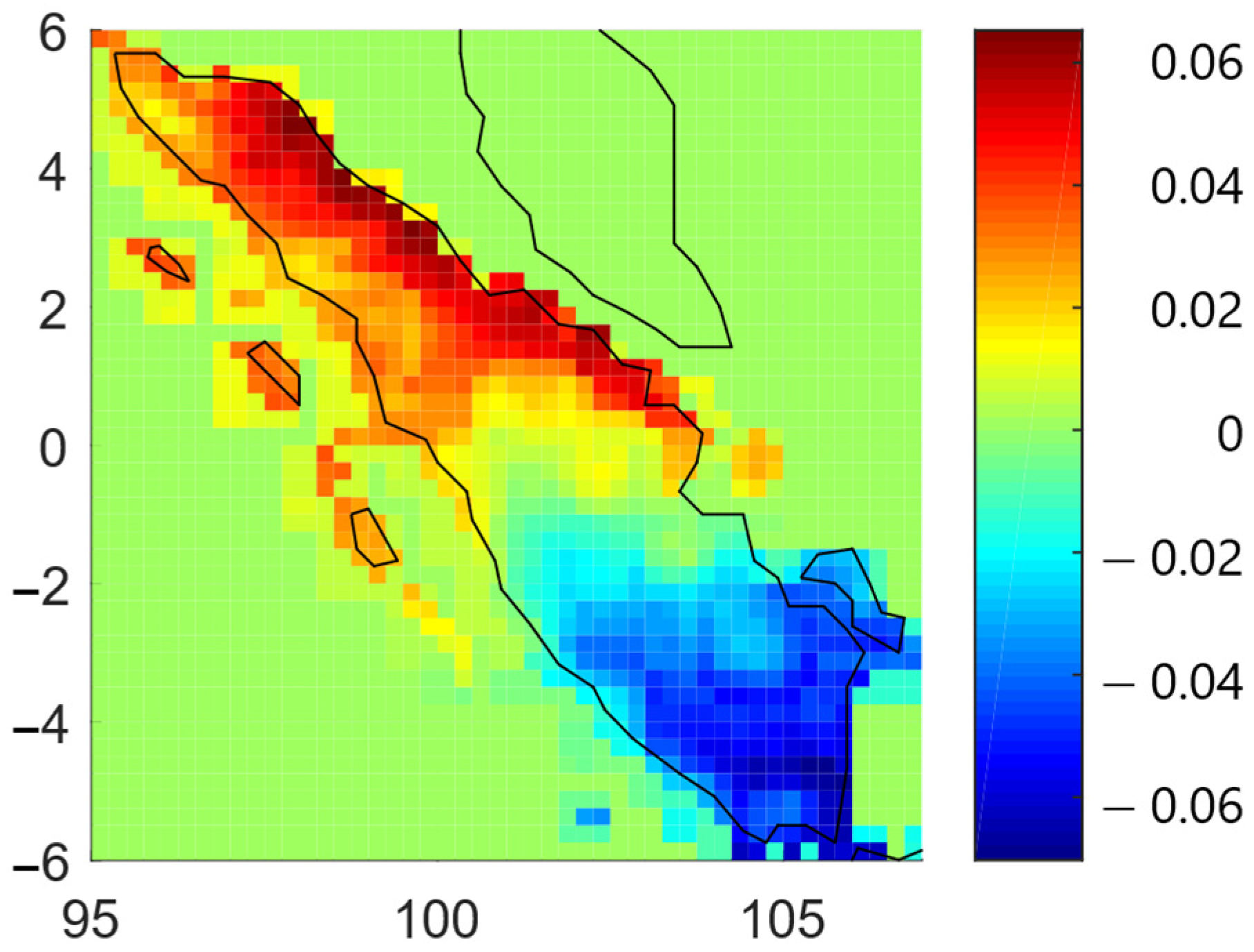
Figure 1. Precipitation types of Sumatra.
Atmosphere 13 00537 g001
Figure 2. Dependency graph of dry spell and precipitation anomaly for 2001–2020 data. The dashed lines represent the separation of wet (bottom/left), normal (middle), and dry (up/right) conditions for dry spell (vertical line) and precipitation anomaly (horizontal line).
Atmosphere 13 00537 g002
Figure 3. Dependency graph of dry spell and hotspot for 2001–2020 data. The dashed lines represent the separation of wet (bottom/left), normal (middle), and dry (up/right) conditions for dry spell (vertical line) and hotspot (horizontal line).
Atmosphere 13 00537 g003
Figure 4. Dependency graph of precipitation anomaly and hotspot for 2001–2020 data. The dashed lines represent the separation of wet (bottom/left), normal (middle), and dry (up/right) conditions for precipitation anomaly (vertical line) and hotspot (horizontal line).
Atmosphere 13 00537 g004
Figure 5. Conditional survival probability of hotspot when the climate (a. dry spell, b. prec. anomaly) conditions are at least in normal conditions and when (c. dry spell, d. prec. anomaly) conditions are in dry conditions for 2001–2020 data.
Atmosphere 13 00537 g005
Figure 6. Dependency graph of each variable pair as well as conditional probability of 5% upper right quadrant from all observed data (January 2001–December 2020) on Sumatra with monsoonal-type precipitation.
Atmosphere 13 00537 g006
Figure 7. Dependency graph of dry spell and precipitation anomaly for 2001–2020 data. The dashed lines represent the separation of wet (bottom/left), normal (middle), and dry (up/right) conditions for dry spell (vertical line) and precipitation anomaly (horizontal line).
Atmosphere 13 00537 g007
Figure 8. Dependency graph of dry spell and hotspot for 2001–2020 data. The dashed lines represent the separation of wet (bottom/left), normal (middle), and dry (up/right) conditions for dry spell (vertical line) and hotspot (horizontal line).
Atmosphere 13 00537 g008
Figure 9. Dependency graph of precipitation anomaly and hotspot for 2001–2020 data. The dashed lines represent the separation of wet (bottom/left), normal (middle), and dry (up/right) conditions for precipitation anomaly (vertical line) and hotspot (horizontal line).
Atmosphere 13 00537 g009
Figure 10. Dependency graph of each variable pair as well as conditional probability of 5% upper right quadrant from all observed data (January 2001–December 2020) on Sumatra with equatorial-type precipitation (2nd dry season: June–September).
Atmosphere 13 00537 g010
Figure 11. Dependency graph of dry spell–prec. anomaly and dry spell–hotspot for 2001–2020 data. The dashed lines represent the separation of wet (bottom/left), normal (middle), and dry (up/right) conditions for dry spell (vertical line) and hotspot (horizontal line).
Atmosphere 13 00537 g011
Figure 12. Conditional survival probability of hotspot when the climate dry spell conditions are at least in a. normal conditions and b. dry conditions for 2001–2020 data.
Atmosphere 13 00537 g012
Figure 13. Dependency graph of each variable pair as well as conditional probability of 5% upper right quadrant from all observed data (January 2001–March 2020) on Sumatra with equatorial-type precipitation (1st dry season: January–March).
Atmosphere 13 00537 g013
Table 1. Cumulative distribution functions and parameter ranges of obtained copula family.
Copula C x ( u 1 , u 2 ) Parameter Range
Gaussian (Normal) F N ( 0 ,   ) ( F N ( 0 , 1 ) 1 ( u 1 ) , F N ( 0 , 1 ) 1 ( u 2 ) )
Clayton ( u 1 θ + u 2 θ 1 ) ( 1 θ ) θ ( 1 , ) ,   θ 0
Frank 1 θ ln [ 1 + w 1 w 2 ( e 1 1 ) ] ; w i = e θ u i 1 θ 0
Gumbel exp [ ( w 1 θ + w 2 θ ) 1 θ ] ; w i = ln ( u i ) θ 1
Student’s t F t ( v ,   ) ( F t ( v ) 1 ( u 1 ) , F t ( v ) 1 ( u 2 ) )
Table 2. Measure of association between each variable pair from 2001–2020 data of Southern Sumatra.
Variable Pair L a n NormalWENMENSENWENPI
Dry spell–Prec. anomaly−0.409−0.394−0.468−0.221−0.709−0.714
Dry spell–Hotspot0.2180.1390.1680.1730.1790.183
Prec. anomaly–Hotspot−0.144−0.137−0.082−0.068−0.067−0.109
Table 3. Measure of association of each variable pair from 2001 to 2020 of 2nd dry season in northern Sumatra.
Variable L a n NormalWENMENSENWENPI
Dry spell–Prec. anomaly−0.217−0.263−0.061−0.119−0.345−0.363
Dry spell–Hotspot0.0550.002−0.0170.022−0.1020.077
Prec. anomaly–Hotspot−0.035−0.060.113−0.071−0.0640
Table 4. Measure of association of each variable pair from 2001 to 2020 of 1st dry season in northern Sumatra.
VariablePhase 1–4Phase 5Phase 6Phase 7Phase 8
Dry spell–Prec. anomaly−0.629−0.6437−0.650−0.700−0.578
Dry spell–Hotspot0.1200.1090.13870.1470.166
Prec. anomaly–Hotspot−0.067−0.062−0.086−0.074−0.104
Publisher’s Note: MDPI stays neutral with regard to jurisdictional claims in published maps and institutional affiliations.