Exploring the Sensitivity of Visibility to PM_2.5 Mass Concentration and Relative Humidity for Different Aerosol Types

Abstract

Fine particle (PM_2.5) mass concentration and relative humidity (RH) are the primary factors influencing atmospheric visibility. There are some studies focused on the complex, nonlinear relationships among visibility, PM_2.5 concentration, and RH. However, the relative contribution of the two factors to visibility degradation, especially for different aerosol types, is difficult to quantify. In this study, the normalized forward sensitivity index method for identifying the dominant factors of visibility was used on the basis of the sensitivity of visibility to PM_2.5 and RH changes. The visibility variation per unit of PM_2.5 or RH was parameterized by derivation of the visibility multivariate function. The method was verified and evaluated based on 4453 valid hour data records in Tianjin, and visibility was identified as being in the RH-sensitive regime when RH was above 75%. In addition, the influence of aerosol chemical compositions on sensitivity of visibility to PM_2.5 and RH changes was discussed by analyzing the characteristics of extinction components ((NH₄)₂SO₄, NH₄NO₃, organic matter, and elemental carbon) measured in Tianjin, 2015. The result showed that the fitting equation of visibility, PM_2.5, and RH, separately for different aerosol types, further improved the accuracy of the parameterization scheme for visibility in most cases.

1. Introduction

Atmospheric horizontal visibility is defined as the distance at which the contrast of a black object with respect to its background is equal to the contrast threshold of human eyesight and is an indicator of atmospheric transparency [1]. Good visibility is a desirable feature of any geographical location, and its importance should be considered [2]. However, many megacities have suffered from air pollution incidents accompanied by a decline in visibility during the past several decades [3,4,5]. Poor visibility severely affects tourism, transportation, and mental health [6,7,8].

Visibility degradation is mainly attributed to light scattering and absorption by atmospheric fine particles [9,10]. There is an obvious, negative correlation between visibility and PM_2.5 concentration [11,12,13,14]. A form of power function or exponential function between visibility and PM_2.5 concentration was observed in many cities [11,15,16]. Notably, when the PM_2.5 concentration was lower than a certain threshold, visibility increased quickly as the PM_2.5 concentration declined [11,16,17,18]. The threshold values of PM_2.5 vary by city. For example, the threshold corresponding to visibility < 10 km in Beijing, Xi’an, and Shanghai is 110, 88, and 65 µg/m³, respectively [11,16,17]. This difference may reduce the reliability of haze event identification when a fixed visibility threshold is employed [19].

Visibility variation shows a clear dependence on relative humidity (RH) also [20,21]. Chen et al. [22] indicated that the decrease in visibility was mainly influenced by RH when RH was >90%. Hygroscopic growth usually increases aerosol extinction coefficients by enlarging the particle size due to the uptake of liquid water. In some other cases, aerosol extinction can be decreased by lowering the refractive index because the refractive index of water is smaller than that of other aerosol components [23]. Positive or negative effects are dictated to a large degree by components [21].

There are complex, nonlinear relationships among visibility, PM_2.5 concentration, and RH, which are deeply affected by the component composition of particles in addition to the mixing state and size distribution [21,24,25,26]. The effect of particles and RH on visibility is further complicated by the differences in extinction abilities of particle components [11,27,28]. Water-soluble, inorganic salts (e.g., (NH₄)₂SO₄, NH₄NO₃) and carbonaceous (e.g., organic matter (OM), elemental carbon (EC) aerosols are the major extinction components in particles with various, dry extinction efficiencies and hygroscopicities [29,30]. The high content of extinction components in particles can increase the sensitivity of visibility to particle concentration. Similarly, the percentage of hygroscopic components (e.g., (NH₄)₂SO₄, NH₄NO₃) in PM_2.5 affects the sensitivity of visibility to RH [10,24]. The content of extinction components in PM_2.5 varies obviously by region and period [8,11,25]. For example, the content of major extinction components ((NH₄)₂SO₄, NH₄NO₃, OM, and EC) and hygroscopic components ((NH₄)₂SO₄ and NH₄NO₃) in PM_2.5 in Shanghai (83% and 42%) was 1.7 times greater than those in Chengdu (48% and 25%, respectively) [31,32]. Thus, identifying the primary factors influencing visibility is essential.

In most cases, atmospheric visibility is affected by both particle concentration and RH; if it is dominated by particulate matter, the effect of emission reduction measures is obvious, but if it is dominated by RH, the same emission reduction measures may not achieve the expected effect. Many studies were conducted to gain insights into correlations between low-visibility events and influencing factors [13,18,30]. However, the sensitivity of visibility to PM_2.5, mass concentration, and RH by aerosol type remains unclear.

In predicting and preventing low-visibility events, determining whether the main cause is PM_2.5 or RH is essential [19,33]. There are some studies focused on the complex, nonlinear relationships among visibility, PM_2.5 concentration, and RH. However, the relative contribution of the two factors to visibility degradation, especially by aerosol type, was difficult to quantify. Thus, this study attempts to build a method for identifying the dominant factors of visibility on the basis of the sensitivity of visibility to PM_2.5 and RH changes. A total of 4453 valid hour data records of visibility, PM_2.5, and RH in Tianjin, 2015, were used to verify and evaluate the method. In addition, aerosols were classified based on the extinction component ((NH₄)₂SO₄, NH₄NO₃, OC, EC, fine soil, and sea salt) measured synchronously online to analyze the influence of aerosol chemical compositions on sensitivity of visibility to PM_2.5 and RH changes.

2. Data and Methods

2.1. The Online Observation of PM_2.5 Chemical Composition and Meteorological Factors

Tianjin (39°100′ N, 117°100′ E) is in the Beijing-Tianjin-Hebei urban agglomeration. It is adjacent to Bohai Bay and has the largest comprehensive port in northern China, the Tianjin Port. The climate is dominated by continental monsoons with distinct seasonal variation and holds the semi-humid characteristic of warm, temperate zones. Sampling instruments used in this study were installed on the rooftop of the Tianjin Eco-Environmental Monitoring Center, approximately 10 m above ground level. The site was expected to reflect the pollution characteristics of a thickly settled urban district.

The mass concentration of PM_2.5 was sampled 1 time every 5 min using a particle monitor (TEOM 1405-F, Thermo Fisher Scientific, Waltham, MA, USA) from February to December 2015. The values measured within an hour were averaged to match with other parameters. The monitor was composed of a filter dynamics measurement system and a tapered element oscillating microbalance mass sensor installed in an individual cabinet. The method detection limit (MDL) was up to 0.1 μg/m³. The inorganic ions (Ca²⁺, Na⁺, NH₄⁺, Cl⁻, NO₃⁻, and SO₄²⁻) of PM_2.5 were synchronously analyzed by an ion-monitoring instrument (AIM URG9000D, Enviro Technology Services, Chapel Hill, NC, USA) with 1 h resolution. The AIM was composed of one particle collection system and two ion chromatographs for anion and cation analyses. The MDLs for Ca²⁺, Na⁺, NH₄⁺, Cl⁻, NO₃⁻, and SO₄²⁻ were 2.3, 0.6, 1.8, 0.2, 0.2, and 0.3 μg/m³, respectively. The 1 h resolution concentration data of carbon components (OC and EC) in PM_2.5 were determined by a semi-continuous OC/EC analyzer (Sunset Laboratory Inc., Portland, OR, USA). The analyzer was calibrated monthly using a blank punch of pre-heated quartz fiber filter and standard sucrose solutions (3.2 mgC/mL) for quality control. The MDLs for OC and EC were 0.45 and 0.06 μg/cm², respectively. The quartz fiber filter was changed weekly during the analysis.

Relative humidity was measured by a VAISALA WST520 automatic weather station with a time resolution of 5 s. The systematic error of relative humidity measurement was within ±3%. Atmospheric visibility was measured using a Belfort 6000 instrument (Belfort Instrument , Belfort, CA, USA), based on forward scattering with a time resolution of 10 min. The systematic error of atmospheric visibility measurement was less than 10%. The visibility values measured within an hour were averaged to match with other parameters. The hourly concentration data for PM_2.5, water-soluble ions, carbon species, RH, and visibility simultaneously were designated as one sample. Instrument failure, bad weather, and other factors led to partial data loss or abnormality. Singular values (e.g., abnormally high values, abnormally low values, and values above the instrument limit or with a large relative standard deviation) were removed. Details on the quality control (QC) of observations were provided in studies [34,35]. This study obtained 4453 samples from Tianjin, 2015, after validation with QC procedures.

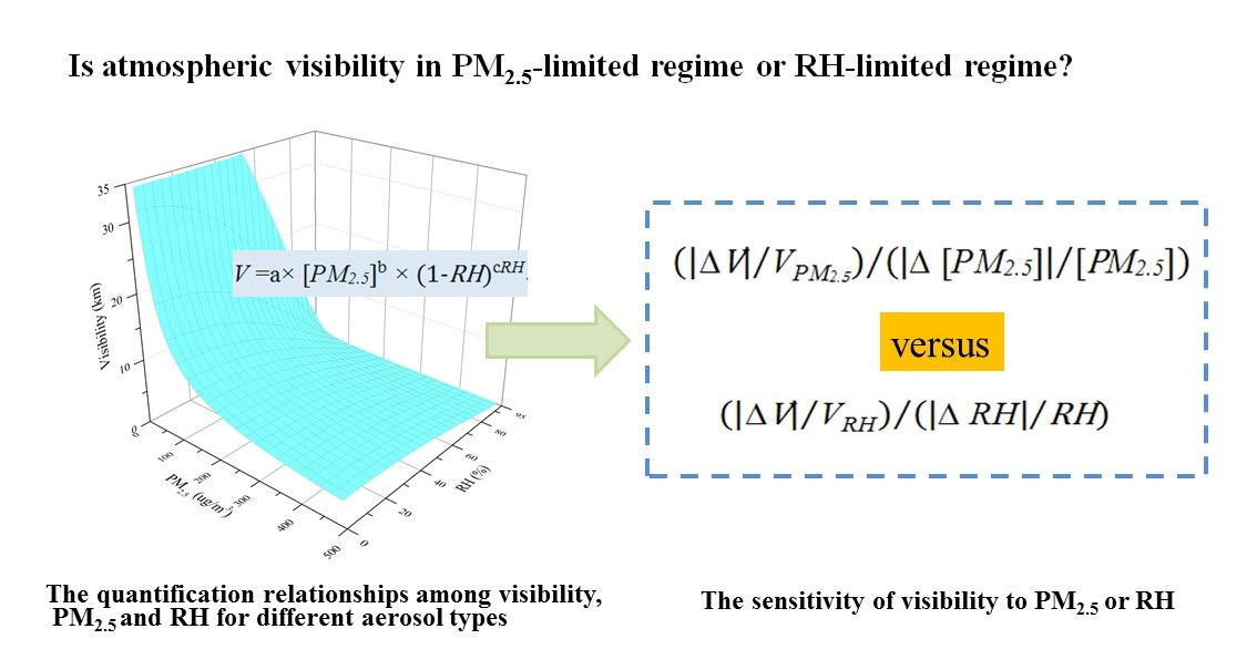
2.2. Parameterization Scheme of Atmospheric Visibility

Many studies found that there is a negative exponential relationship, as shown in Equation (1) [11,36]. Considering the influence of aerosol hygroscopic growth on visibility, RH was selected as another factor for visibility parameterization. Song et al. [36] found that there was a power relationship between RH and visibility, and the function was combined with Equation (1) to simulate visibility (Equation (2)). Another equation, Equation (3), evolved by multiplying the power function between extinction coefficient and aerosol concentration and the empirically power-exponential function between extinction coefficient and RH [22,37,38]. All variables could be easily acquired; thus, the parameterization was practical.

$$V=f\left(x\right)=\mathrm{a}\times \exp (\mathrm{b}\times x)+\mathrm{c}$$

(1)

where the visibility is a function of one parameter, PM_2.5: f(x); V and x are visibility and PM_2.5 with units of km and μg/m³, respectively; and parameters a, b, and c are the regression coefficients of the schemes.

$${V=f(x,y)=\mathrm{a}\times \exp (\mathrm{b}\times x)+\mathrm{c}\times y}^d+\mathrm{e}$$

(2)

where the visibility is a function of two parameters, PM_2.5 and RH: f(x,y); V, x, and y are visibility, PM_2.5, and RH with units of km, μg/m³, and %, respectively; and parameters a, b, c, d, and e are the regression coefficients of the schemes.

$${V=f(x,y)=\mathrm{a}\times x}^b\times {\left(1-y\right)}^{c·y}$$

(3)

where the visibility is a function of two parameters, PM_2.5 and RH: f(x,y); V, x, and y are visibility, PM_2.5, and RH with units of km, μg/m³, and %, respectively; and parameters a, b, and c are the regression coefficients of the schemes.

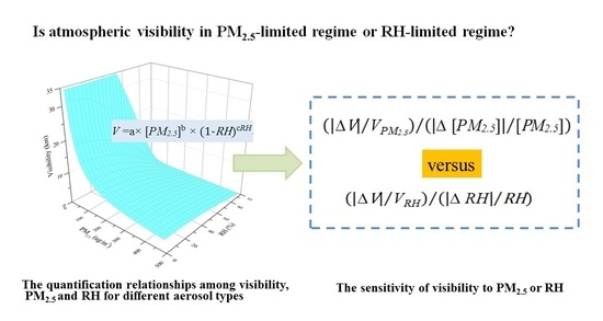
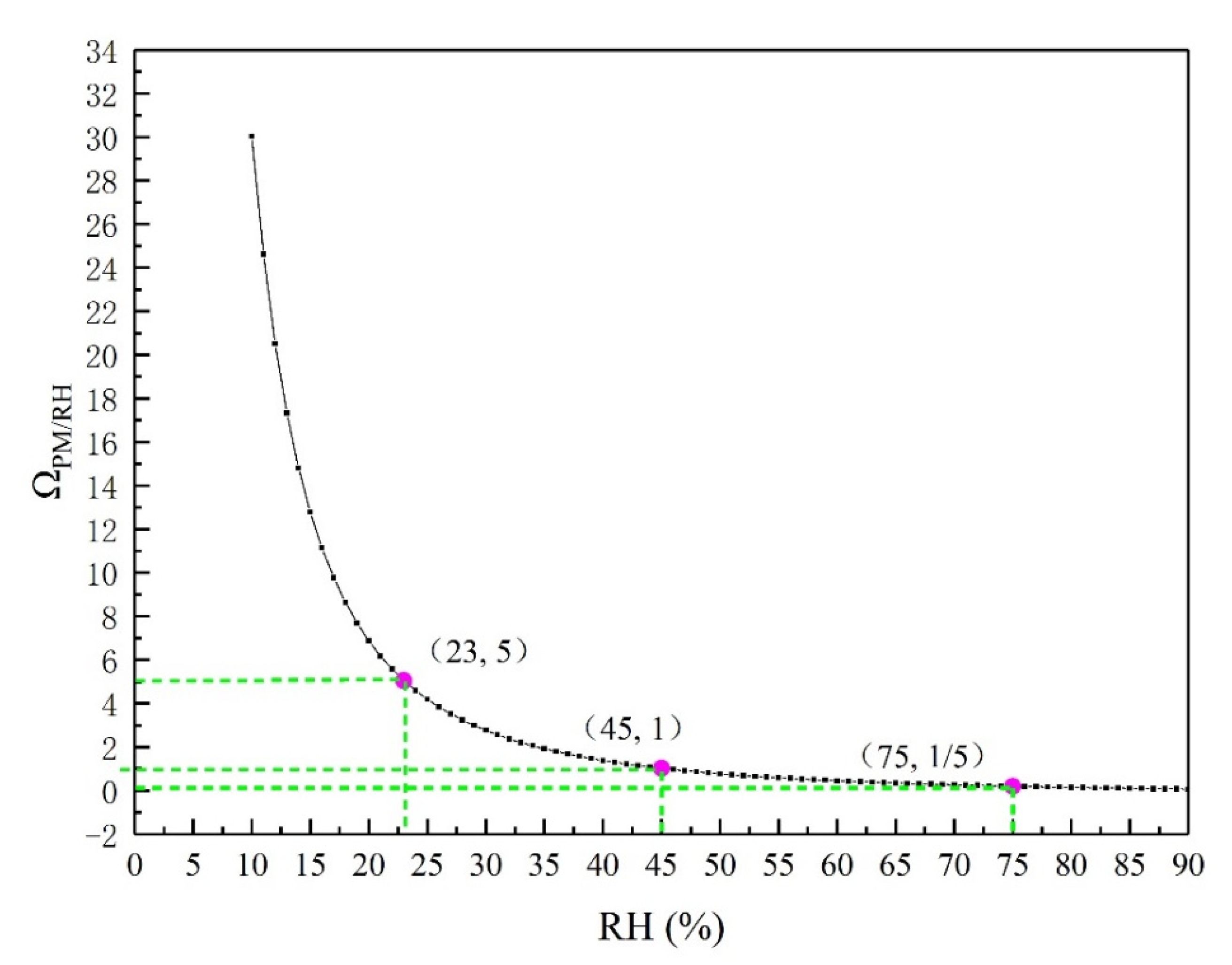
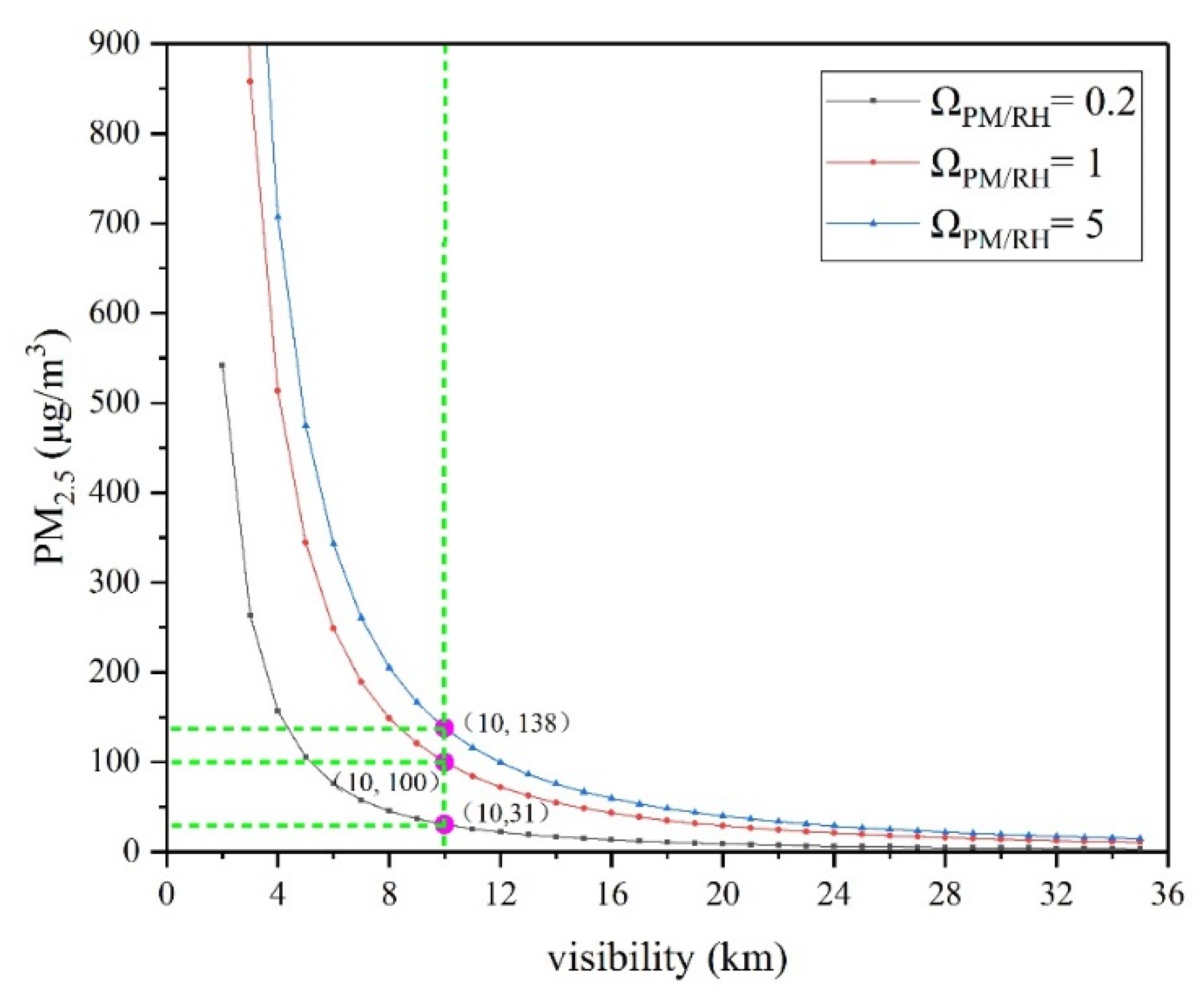
2.3. Classification Method of Visibility-Sensitive Regime, Depending on the Sensitivity of Visibility to PM_2.5 Concentration and RH

To test the sensitivity of visibility to PM_2.5 concentration and RH, the normalized forward sensitivity index method [19,39,40] was used, shown as Equations (4) and (5). The normalized forward sensitivity index (K_V-R) of a variable (PM_2.5 concentration or RH) to visibility is the ratio of the relative change in the variable to the relative change in the visibility.

$$K_{{V-PM}2.5}=(|\Delta V_{x_i}|/V_{x_i})/\left(\left|\Delta x_i\right|/x_i\right)=|\Delta V_{x_i}/\Delta x_i|{\times x}_i{/V}_{x_i}$$

(4)

where V is visibility with units of km; x is PM_2.5 with units of μg/m³; and y is RH with units of %; $x_i$ is the different level of PM_2.5 concentrations, i = 1, 2, 3……m; $\Delta x_i$ is the variation of $x_i$;$V_{x_i}$is the visibility under the i level of PM_2.5 concentration; $\Delta V_{x_i}$ is the visibility variation caused by $\Delta x_i$; and $K_{{V-PM}2.5}$ is the sensitivity index of visibility under the i level of PM_2.5 concentration.

$$K_{V-RH}=\left(\right|\Delta V_{y_j}|/V_{y_j})/\left(\left|\Delta y_j\right|/y_j\right)=|\Delta V_{y_j}/\Delta y_j|{\times y}_j{/V}_{y_j}$$

(5)

where V, x, and y are visibility, PM_2.5, and RH with units of km, μg/m³, and %, respectively. $y_j$ is the different level of RH, j = 1, 2, 3……n; $\Delta y_j$ is the variation of RH at value $y_j$;$V_{y_j}$is the visibility under the j level of RH; $\Delta V_{y_j}$is the visibility variation caused by $\Delta y_j$; and $K_{V-RH}$ is the sensitivity index of visibility under the j level of RH.

When the variable is a differentiable function of the parameter, the sensitivity index may be alternatively defined using partial derivatives. There is a functional relationship among visibility, PM_2.5, and RH, shown as Equations (1)–(3) in this study. $K_{{V-PM}2.5}$ and $K_{V-RH}$ can be approximately expressed as Equations (6) and (7):

$$|\Delta V_x/\Delta x|\approx {|f\text{’}}_x(x,y)|$$

(6)

$$|\Delta V_y/\Delta y|\approx {|f\text{’}}_y(x,y)|$$

(7)

where V is visibility with units of km; x is PM_2.5 with units of μg/m³; and y is RH with units of %; $f(x,y)$ is the parameterization scheme of visibility, PM_2.5 concentration, and RH obtained in Section 2.2; ${f\text{’}}_x(x,y)$and ${f\text{’}}_y(x,y)$are partial derivatives of$f\left(x,y\right)$, respectively.

Visibility relative sensitivity index${\mathsf{\Omega }}_{PM/RH}$ is defined as Equation (8):

$${\mathsf{\Omega }}_{PM/RH}=K_{{V-PM}2.5}/K_{V-RH}$$

(8)

where $K_{{V-PM}2.5}$ and $K_{V-RH}$ is the sensitivity index of visibility to PM_2.5 concentration and RH, respectively; and ${\mathsf{\Omega }}_{PM/RH}$ is the ratio of visibility variation per unit of PM_2.5 to RH.

When ${\mathsf{\Omega }}_{PM/RH}=1$, the effects of the concentration of PM_2.5 and RH on visibility is similar. When the ratio is greater than one, indicating that visibility is more sensitive to PM_2.5 than RH, visibility is identified as being in the PM_2.5-sensitive regime. When${\mathsf{\Omega }}_{PM/RH}$ is lower than 1, the visibility variation caused by the increase in RH is greater than that caused by particle concentration, and visibility is identified as being in the RH-sensitive regime. The classification method of visibility for different control categories was used to identify the main influencing factors by determining the threshold of aerosol mass concentration and RH.

2.4. IMPROVE Equations

In this study, the extinction contribution of the composition of fine particles to visibility degradation was investigated using the Interagency Monitoring of Protected Visual Environments (IMPROVE) equation, an extensively used method for estimating the light extinction coefficient based on aerosol chemical composition [41,42]. Equation (9) is the revised IMPROVE algorithm in which coarse particulate, NO₂, and Rayleigh scattering were excluded because of the low contributions [42,43].

$$\begin{gathered} {\mathrm{B}}_{ext}\approx 2.2\times f_S\left(RH\right)*\left[Small{\left({NH}_4\right)}_2{SO}_4\right]+4.8\times f_L\left(RH\right)*\left[Large{\left({NH}_4\right)}_2{SO}_4\right]+ \\ 2.4\times f_S\left(RH\right)*\left[Small{\left({NH}_4\right)}_2{SO}_4\right]+5.1\times f_L\left(RH\right)*\left[Large{\left({NH}_4\right)}_2{SO}_4\right]+2.8\times \left[SmallOM\right]+ \\ 6.1\times \left[LargeOM\right]+10\times \left[EC\right]+1\times \left[FineSoil\right]+1.7\times f_{SS}\left(RH\right)\times \left[SeaSalt\right] \end{gathered}$$

(9)

where [(NH4)₂SO₄], [NH₄NO₃], [OM], [EC], $\left[FineSoil\right]$, and $\left[SeaSalt\right]$ are the concentrations of (NH₄)₂SO₄, NH₄NO₃, OM (organic matter), EC, fine soil, and sea salt in units of μg/m³; $B_{ext}$ is the light extinction coefficient of aerosol, Mm⁻¹. The fraction of the fine particle component ((NH4)₂SO₄, NH₄NO₃, or OM) that is in the large mode is estimated by dividing the total concentration of the component by 20 μg/m³. The coefficient of the equation is the dry mass extinction efficiency of each extinction component, which represents the light scattering or absorption extinction coefficient under the unit mass concentration. $f_S$(RH), $f_L$(RH), and $f_{SS}\left(RH\right)$ is the hygroscopic growth factor of small- and large-mode ammonium salt and sea salt, determined according to the measured RH [42].

Most of the sulfate, nitrate, and organic carbon in the particles are in the form of (NH₄)₂SO₄, NH₄NO₃, and OM, respectively [44]. The average equivalent concentrations of NH₄⁺, SO₄²⁻, NO₃⁻ measured in this study were 0.69, 0.13, and 0.22 μeq/m³, respectively. There was sufficient NH₄⁺ to match SO₄²⁻ and NO₃⁻. Therefore, the concentrations of (NH₄)₂SO₄ and NH₄NO₃ were reconstructed based on Equations (10) and (11). OM was estimated by multiplying the OC by 1.6, which is suitable for urban aerosol (Equation (12)) [42,45]. Sea salt mass was calculated based on the concentrations of Na⁺ and Cl⁻ (Equation (13)) [44]. Fine soil mass was assumed to be 20 times of that of Ca²⁺ based on previous soil source profiles (Equation (14)) [46,47,48].

$$\left[{\left({NH}_{\mathit{4}}\right)}_{\mathit{2}}{SO}_{\mathit{4}}\right]=1.29\left[{{SO}_4}^{2-}\right]$$

(10)

where [SO₄²⁻] and [(NH₄)₂SO₄] are the concentrations of SO₄²⁻ and (NH₄)₂SO₄ in units of μg/m³.

$$\left[{NH}_{\mathit{4}}{NO}_{\mathit{3}}\right]=1.375\left[{NO}_{3^{-}}\right]$$

(11)

where [NO₃⁻] and [NH₄NO₃] are the concentrations of NO₃⁻ and NH₄NO₃ in units of μg/m³.

$$\left[OM\right]=1.6\left[OC\right]$$

(12)

where [OC] and [OM] are the concentrations of OC and OM in units of μg/m³.

$$\left[SeaSalt]=1.47\left[{Na}^{+}\right]+[{Cl}^{-}\right]$$

(13)

where [$SeaSalt$], $\left[{Na}^{+}\right]$ and [Cl⁻] are the concentrations of $seasalt$, ${Na}^{+}$, and Cl⁻ in units of μg/m³.

$$\left[FineSoil\right]=20\left[{Ca}^{2+}\right]$$

(14)

where [Fine Soil] and [Ca²⁺] are the concentrations of fine soil and Ca²⁺ in units of μg/m³.

3. Results and Discussion

3.1. Application of Visibility Control Category Classification Method

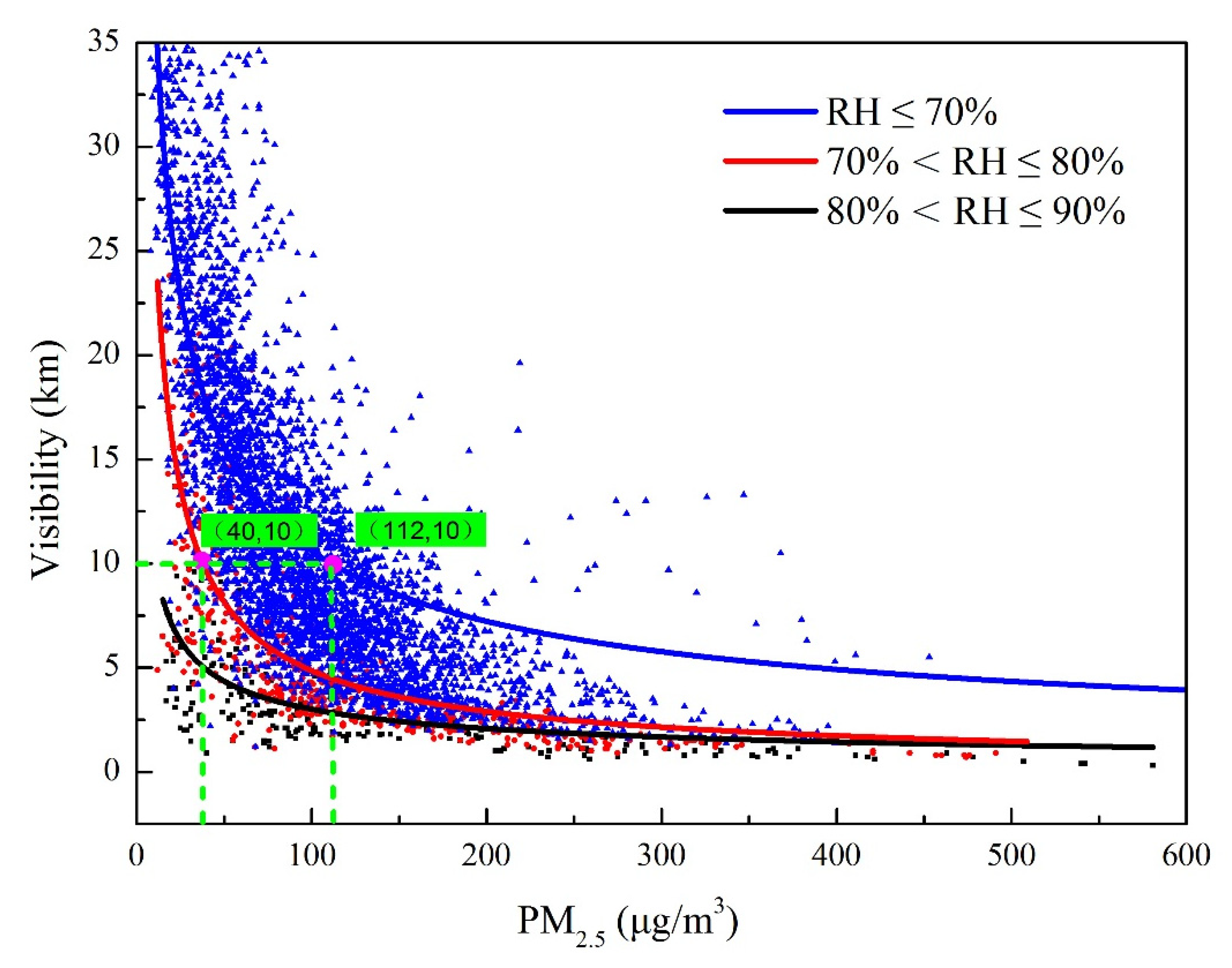
3.1.1. Quantification of Relationships among Visibility, PM_2.5 Concentration, and RH in Tianjin, 2015

Visibility varied from 0.3 to 35.0 km, with an average of 12.0 ± 9.1 km, from February to December 2015 in Tianjin. The average mass concentration of PM_2.5 was 106.0 ± 81.2 μg/m³, and the average RH was 46 ± 21%. There was a strong, negative correlation among visibility and PM_2.5 (−0.64) and RH (−0.67). There was an exponential or power function among visibility, PM_2.5, and RH (Figure 1). The visibility decreased as PM_2.5 increased in different RH ranges. There was a threshold for the sensitivity of visibility and PM_2.5. Under dry conditions (23% ≤ RH < 70%), the threshold of PM_2.5, corresponding to a visibility of 10 km, was 112 μg/m³; however, under an RH of 70–80%, this threshold was lowered to 40 μg/m³. Visibility was almost lower by 10 km when RH was 80–90%. A nonlinear correlation was observed between visibility and PM_2.5, which was affected by RH in most cases [49]. However, the relationship between visibility and PM_2.5 was not dependent on RH at higher concentrations and higher RH, because the black and red lines overlap at higher concentrations.

The relationship among visibility, PM_2.5 concentration, and RH was investigated and quantified based on hourly data obtained from Tianjin, 2015, and 4453 valid datasets were used in the regression analysis (Equations (1)–(3)). The F-test was applied with a confidence level of 95% (α = 0.05). The regression coefficients for the three parameterization schemes are listed in Table S1 in Supplementary Materials. To test the reliability, this study compared the V calculated from the regression and the measured visibilities (Figure 2). The determination R² of Equation (3) at a confidence level of 95% was higher than that of the other two equation forms (0.72 vs. 0.55 and 0.55). The slope of measured and calculated visibility by Equation (3) (0.67) was closer to 1 than these of Equations (1) and (2) (0.55 and 0.55). This result reveals that the compound form of the power and power-exponential function can increase the accuracy of the parameterization scheme for visibility calculation (Equation (15)) in Tianjin, 2015.

$$V=f(x,y)=166.1{\times x}^{-0.56}\times (1-y{)}^{0.86y}$$

(15)

where the visibility is a function of two parameters, PM_2.5 and RH: f(x,y); V was the visibility, varying in the range of 0.3–34.7 km; x was the PM_2.5 concentration, varying in the range of 13–581 μg/m³; and y was the RH, varying in the range of 4–90% in this study.

3.1.2. Sensitivity of Visibility to PM_2.5 Concentration and RH

The parameterization scheme of visibility in Tianjin, 2015 (Equation (15)), was incorporated into Equations (6) and (7) (Section 2.3). At the same PM_2.5 ($x_i$) and RH ($y_j$) points,$V_{x_i}$ was equal to $V_{y_j}$. The visibility relative sensitivity index $\left({\mathsf{\Omega }}_{PM/RH}\right)$ in Tianjin, 2015, was calculated using Equations (16)–(18).

$$K_{{V-PM}2.5}=(-93.01)\times {x_i}^{-0.56}{\times (1-y}_j{)}^{0.86y_j}/V_{x_i}$$

(16)

$$K_{V-RH}=142.84{\times x}_i{}^{-0.56}{\times y}_j{\times (1-y}_j{)}^{0.86y_j}{\times \left[ln\right(1-y}_j{)-y}_j/{(1-y}_j\left)\right]/V_{y_j}$$

(17)

$${\mathsf{\Omega }}_{PM/RH}=(-0.65)/\{y_j{\times \left[ln\right(1-y}_j{)-y}_j/{(1-y}_j\left)\right]\}$$

(18)

where V, x, and y are visibility, PM_2.5, and RH with units of km, μg/m³, and %, respectively; $x_i$ is the different level of PM_2.5 concentrations, i = 1, 2, 3……m;$V_{x_i}$is the visibility under the i level of PM_2.5 concentration;$y_j$ is the different level of RH, j = 1, 2, 3……n; $V_{y_j}$is the visibility under the j level of RH; $K_{V-RH}$ is the sensitivity index of visibility under the j level of RH; $K_{{V-PM}2.5}$ and $K_{V-RH}$ is the sensitivity index of visibility to PM_2.5 concentration and RH, respectively; ${\mathsf{\Omega }}_{PM/RH}$ is the ratio of visibility variation per unit of PM_2.5 to RH.

As shown in Figure 3, ${\mathsf{\Omega }}_{PM/RH}$ decreased as RH increased. When RH was 45%, ${\mathsf{\Omega }}_{PM/RH}$ was equal to one. The influence of PM_2.5 and RH on visibility was similar. When RH was lower than 45%, especially under 23% (${\mathsf{\Omega }}_{PM/RH}$ = 5), ${\mathsf{\Omega }}_{PM/RH}$ increased sharply with the decrease in RH. Thus, visibility was mainly influenced by PM concentration, and visibility was defined as being in the PM_2.5-sensitive regime. At an RH above 75% (${\mathsf{\Omega }}_{PM/RH}$= 0.2), ${\mathsf{\Omega }}_{PM/RH}$ was close to zero and did not change. It means that RH was gradually becoming the main factor influencing visibility, and visibility was identified as being in the RH-sensitive regime when RH was above 75%.

The values of 0.6, 1, 5, 10, and 15 km of visibility are the key points that refer to the classification of dense fog, fog, mist, haze, and good days. By combining Equations (15) and (18), the PM_2.5 and RH threshold values of visibility of different control categories for the above levels were determined respectively. When ${\mathsf{\Omega }}_{PM/RH}$= 1, RH was 45% and PM_2.5 was 345, 100, and 48 μg/m³, corresponding to visibility at 5, 10, and 15 km, respectively (Figure 4).

When visibility was in the PM_2.5-sensitive regime (${\mathsf{\Omega }}_{PM/RH}$= 5), the threshold of RH was 23% and PM_2.5 was 475, 138, and 67 μg/m³, corresponding to visibility at 5, 10, and 15 km, respectively. When visibility was in the RH-sensitive regime (${\mathsf{\Omega }}_{PM/RH}$= 0.2), the threshold of RH was 75% and PM_2.5 was 106, 31, and 15 μg/m³, corresponding to visibility at 5, 10, and 15 km, respectively. When RH was >75%, visibility was more sensitive to the variation in RH than to the increase in PM_2.5. The threshold values of PM_2.5 were out of the observation values measured in this study (581 μg/m³) at 0.6 and 1 km level of visibility, meaning that it is hard for the contribution of particulate matter to exceed the relative humidity during dense fog and fog days.

The result shows that the classification method of visibility control categories built in this study can be used to identify the dominant factors of atmospheric visibility. The precondition was that there was a linear or nonlinear relationship among atmospheric visibility, PM_2.5, and RH, and the relationships were well fitted.

3.2. Sensitivity of Visibility to PM_2.5 Concentration and RH for Different Aerosol Types

PM_2.5 and RH were the main influencing factors on visibility, and a well-fitted parameterization scheme of visibility was provided in this study (Equation (15)). This new model could be applicable and easily transferrable to other datasets worldwide. However, there remained certain deviations between the calculated and measured visibilities (R² = 0.72; slope = 0.67) due to the difference in the aerosol extinction component.

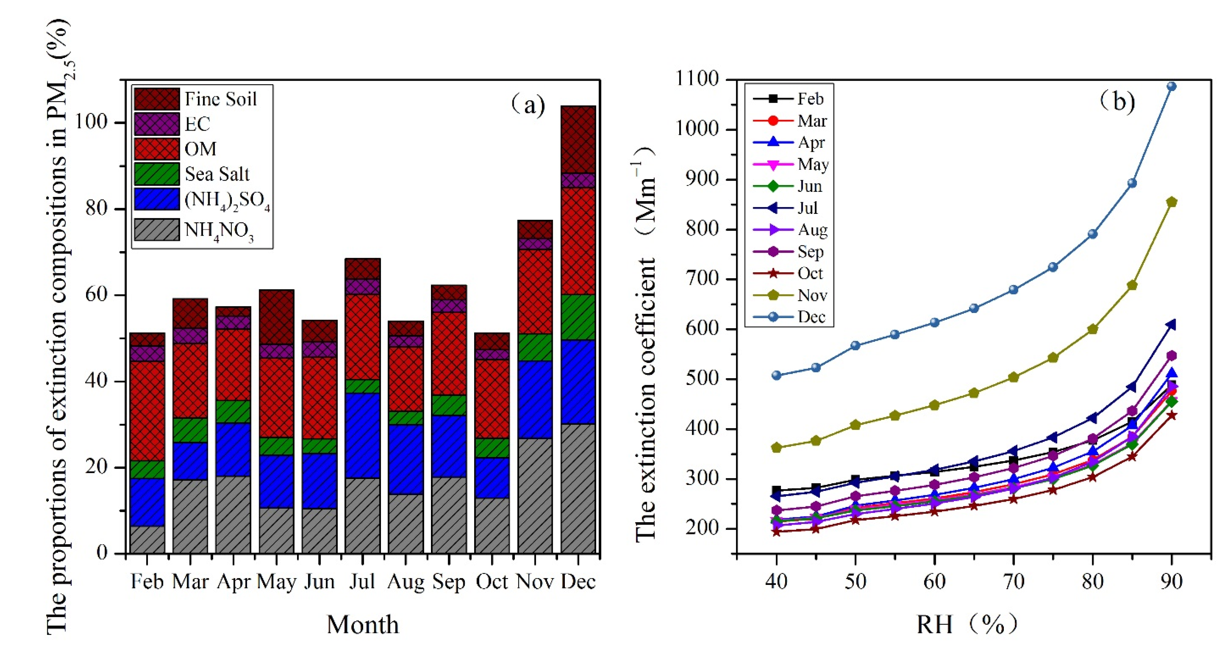
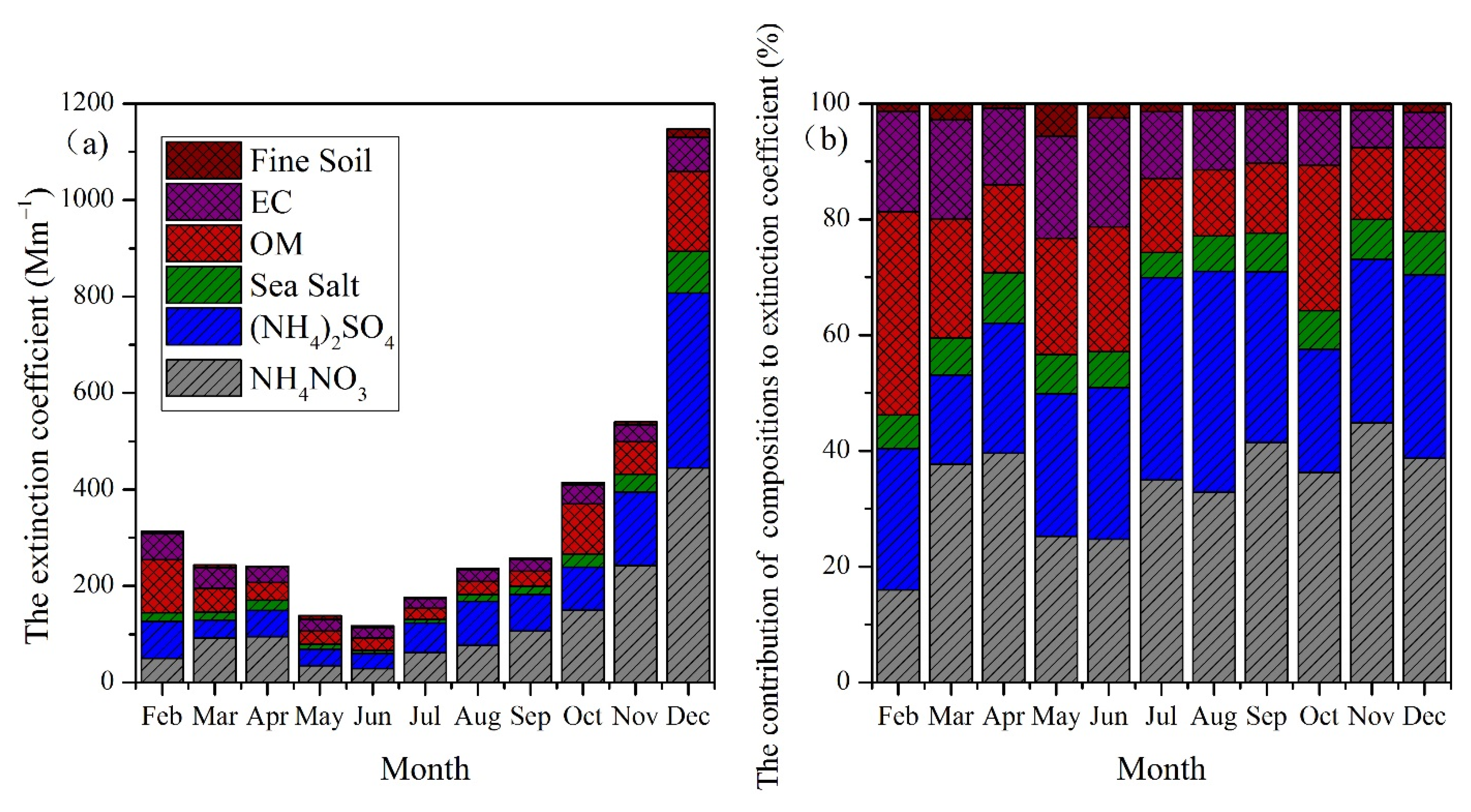
3.2.1. Constituents and Extinction Characteristics of Chemical Composition in PM_2.5

Hourly concentrations of extinction compositions, such as (NH₄)₂SO₄, NH₄NO₃, OM, fine soil, and sea salt, were reconstructed based on Equations (10)–(14). The extinction contribution of the compositions to visibility degradation was investigated using the revised IMPROVE equation (Equation (9)). The correlation coefficient between the extinction coefficient calculated by the IMPROVE equations and visibility (Equation (19), Koschmieder’s law) reached 0.88. The aerosol extinction coefficient calculated by the IMPROVE equations was highest in December (1147.4 Mm⁻¹) and lowest in June (117.0 Mm⁻¹), shown in Figure 5a. The difference was by up to 10 times. The primary extinction components were different in different months (Figure 5b). The contribution of hygroscopic compositions (NH₄NO₃, (NH₄)₂SO₄, and sea salt) to extinction coefficient was up to 80% in November, while it was only 46% in February. The contribution of OM to extinction was highest in February (35%), followed by October (25%), June (31%), and March (30%).

$${\mathrm{B}}_{ext}=k/V\times 1000$$

(19)

where ${\mathrm{B}}_{ext}$ is the light extinction coefficient of aerosol, Mm⁻¹; V is visibility, km; and k is assumed to be 1.97 when the visibility is < 10 km. Otherwise, k is assumed to be 3.912 [46,50].

The annual average proportions of (NH₄)₂SO₄, NH₄NO₃, OM, EC, fine soil, and sea salt in PM_2.5 were 14%, 17%, 19%, 3%, 6%, and 5%, respectively. The proportions of extinction compositions in PM_2.5 changed obviously with the seasons. The monthly average proportions of extinction compositions in PM_2.5 are shown in Figure 6a. In December, November, and July, the major components accounted for the highest proportion of PM_2.5: 104%, 77%, and 68%, respectively. The proportions of major extinction compositions in PM_2.5 were lowest in February (51%) and October (51%). The content difference in the extinction component in PM_2.5 for different seasons could reach up to 2.0 times. The hygroscopic compositions of PM_2.5 accounted for the highest proportion in December (60%), followed by November (51%) and July (40%). These results suggest that constituents of the extinction composition in PM_2.5 differed by period.

To explore the influence of composition constituents on aerosol extinction, this study used the monthly average proportions of (NH₄)₂SO₄, NH₄NO₃, OM, EC, fine soil, and sea salt to calculate extinction coefficients with the IMPROVE equation under the same level of PM_2.5 mass concentration (100 µg/m³) and RH (Figure 6b). The extinction coefficients of aerosols in December were twice that of aerosols in June, even though the PM_2.5 and RH were same. This result was observed because particles with more extinction components were more efficient light scatterers and absorbers.

In February, the sum of major extinction components accounted for 53% of PM_2.5 and was similar to the 54% in August. However, the content of hygroscopic components in August (33%) was higher than that in February (22%). At low RH, the extinction coefficient in February was higher than that in March. With the increase in RH, the growth rate of the extinction coefficient in August was faster than that in February, and it was higher than that in February when RH was more than 85% (Figure 6b). The extinction coefficient of aerosol was more sensitive to RH when the content of hygroscopic components was higher.

In summary, the total content of the extinction components in the particles was the main factor affecting the extinction ability of aerosols, and the content of the hygroscopic components played a critical role in affecting their sensitivity to RH.

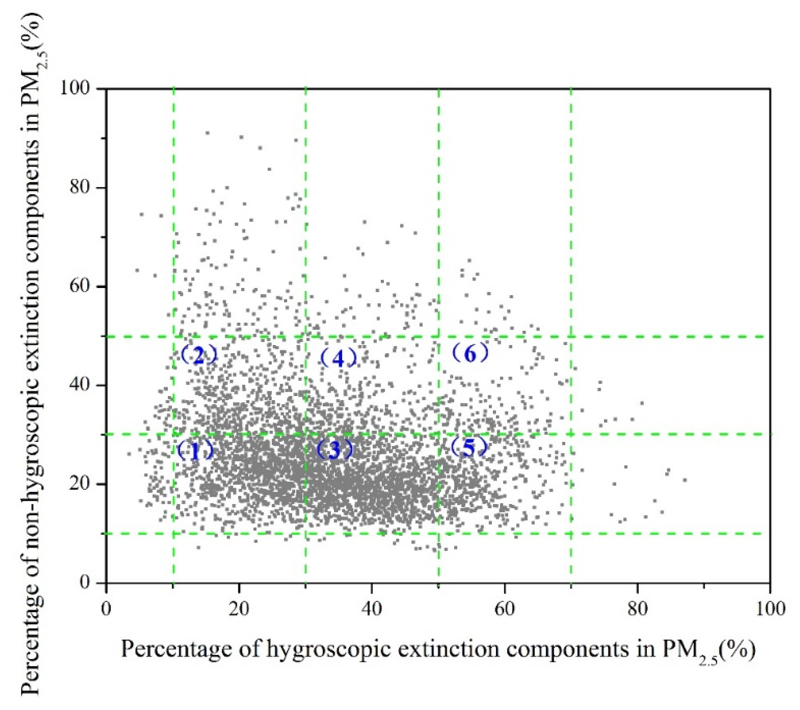
3.2.2. Classification of Aerosol Types

The relationships among visibility, PM_2.5, and RH depended on the extinction capacity of the aerosol composition to a certain extent. In this study, a new aerosol classification method was established based on the percentages of hygroscopic (NH₄NO₃, (NH₄)₂SO₄, and sea salt) and non-hygroscopic (OM, EC, and fine soil) components in PM_2.5, shown as Equations (20) and (21):

$$P_{hyg}{=P}_{{\left({NH}_4\right)}_2{SO}_4}{+P}_{{NH}_4{NO}_3}{+P}_{SS}$$

(20)

$$P_{no-hyg}{=P}_{OM}{+P}_{EC}{+P}_{FS}$$

(21)

where $P_{({\left({NH}_4\right)}_2{SO}_4}$, $P_{{NH}_4{NO}_3}$, $P_{SS}$, $P_{OM}$, $P_{EC}$, $P_{FS}$, $P_{hyg}$, and $P_{no-hyg}$ are the percentages of NH₄NO₃, (NH₄)₂SO₄, sea salt, OM, EC, fine soil, hygroscopic, and non-hygroscopic extinction components in PM_2.5, respectively.

The percentages of hygroscopic and non-hygroscopic extinction components concentrated mainly on the range of 10–70% and 10–50%, shown in Figure 7. A total of 4008 aerosol samples (accounting for 90% of all samples) were classified into six types according to the numerical value of $P_{hyg}$ and $P_{no-hyg}$. At the same particle concentration level, the higher the $P_{hyg}+P_{no-hyg}$ was, the more sensitive the visibility was to the change in the fine particle concentration. The higher the $P_{hyg}$ was, the more sensitive the visibility was to the change in RH.

The characteristics and sample size of the six aerosol types are shown in Table S2. The sample size of aerosols with a low (types 1 and 2) and medium (types 3 and 4) content of hygroscopic components was similar, accounting for 35% and 41%, respectively. Aerosols with a high content of hygroscopic components (types 5 and 6) made up 14%. The content of non-hygroscopic extinction components (types 1, 3, and 5) in most samples (68%) was lower than 30%. Of the aerosols, 22% were in types 2, 4, and 6 with a medium content of non-hygroscopic extinction components. A good correlation between visibility and PM_2.5 was found for different aerosol types with the correlation coefficient varying from −0.54 to −0.71. The correlation coefficient between visibility and RH increased from −0.16 to −0.70 with the increase of the content of hygroscopic components.

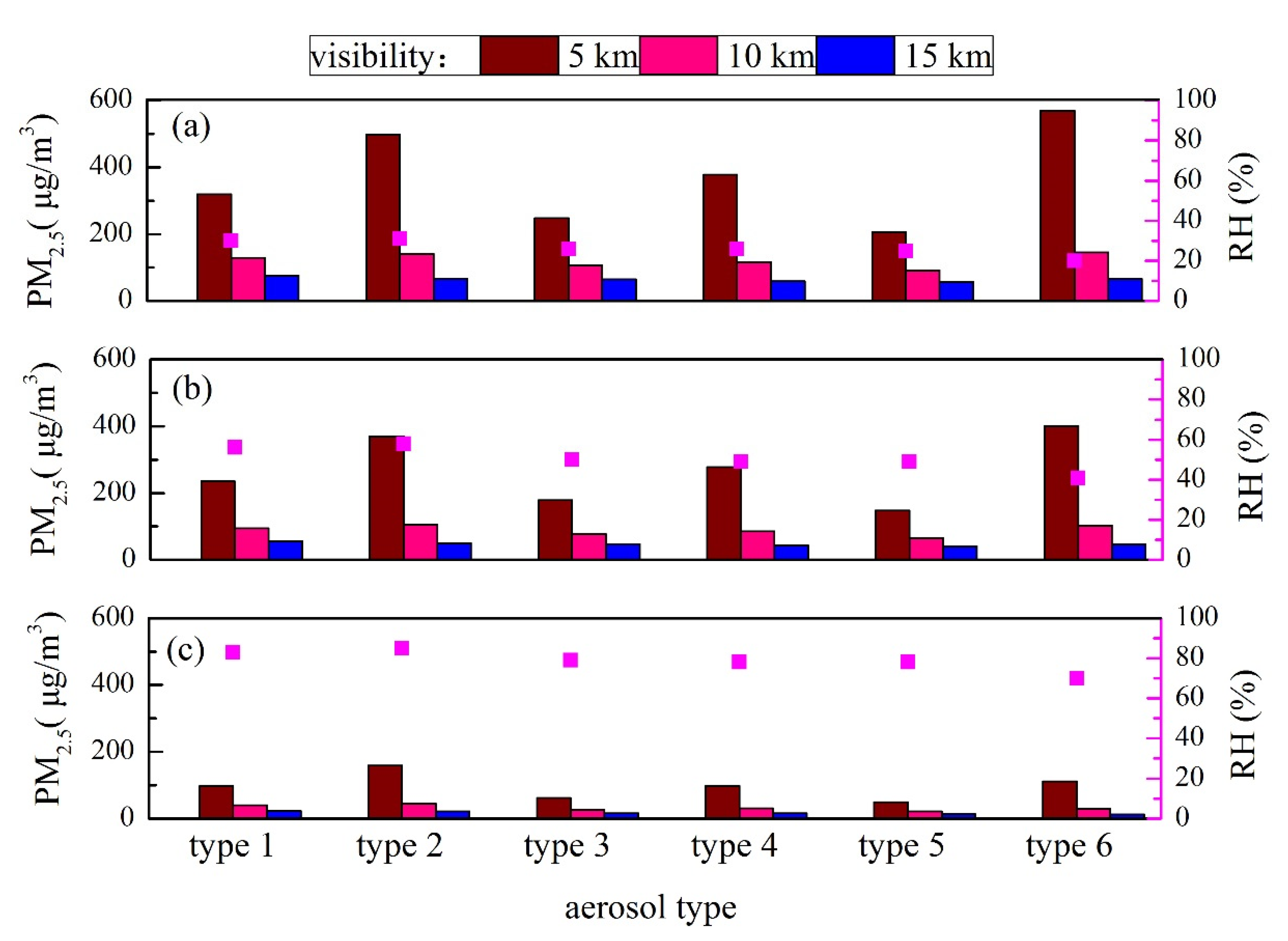
3.2.3. Impacts of Chemical Compositions on the Sensitivity of Visibility to PM_2.5 and RH

The varied correlation among visibility, PM_2.5, and RH for different aerosol types indicated that the content of chemical compositions greatly influences the sensitivity of visibility to PM_2.5 and RH. In this study, the quantitative relationship among visibility, PM concentration, and RH in different aerosol types was fitted based on Equations (1)–(3).FS The compound form of the power and power-exponential function was still identified as the optimal fit among visibility, PM_2.5, and RH (Equation (3)). Coefficients and fitting effects varied by aerosol type (

Table 1. Fitting equation and effect of visibility, PM_2.5, and RH for different aerosol types.

Type	Fitting Equation	Relationship between Measured and Calculated Visibility	R2
1	$V=447.9\times {\left[{PM}_{\mathit{2.5}}\right]}^{-0.77}\times {\left(1-RH\right)}^{0.67·RH}$	y = 0.62x + 4.66	0.65
2	$V=159.4\times {\left[{PM}_{\mathit{2.5}}\right]}^{-0.55}\times {\left(1-RH\right)}^{0.42·RH}$	y = 0.64x + 5.83	0.66
3	$V=496.6\times {\left[{PM}_{\mathit{2.5}}\right]}^{-0.82}\times {\left(1-RH\right)}^{0.99·RH}$	y = 0.75x + 1.93	0.76
4	$V=176.7\times {\left[{PM}_{\mathit{2.5}}\right]}^{-0.59}\times {\left(1-RH\right)}^{0.72·RH}$	y = 0.61x + 4.58	0.64
5	$V=491.9\times {\left[{PM}_{\mathit{2.5}}\right]}^{-0.85}\times {\left(1-RH\right)}^{1.08·RH}$	y = 0.84x + 0.65	0.84
6	$V=132.4\times {\left[{PM}_{\mathit{2.5}}\right]}^{-0.51}\times {\left(1-RH\right)}^{1.04·RH}$	y = 0.72x + 1.90	0.76
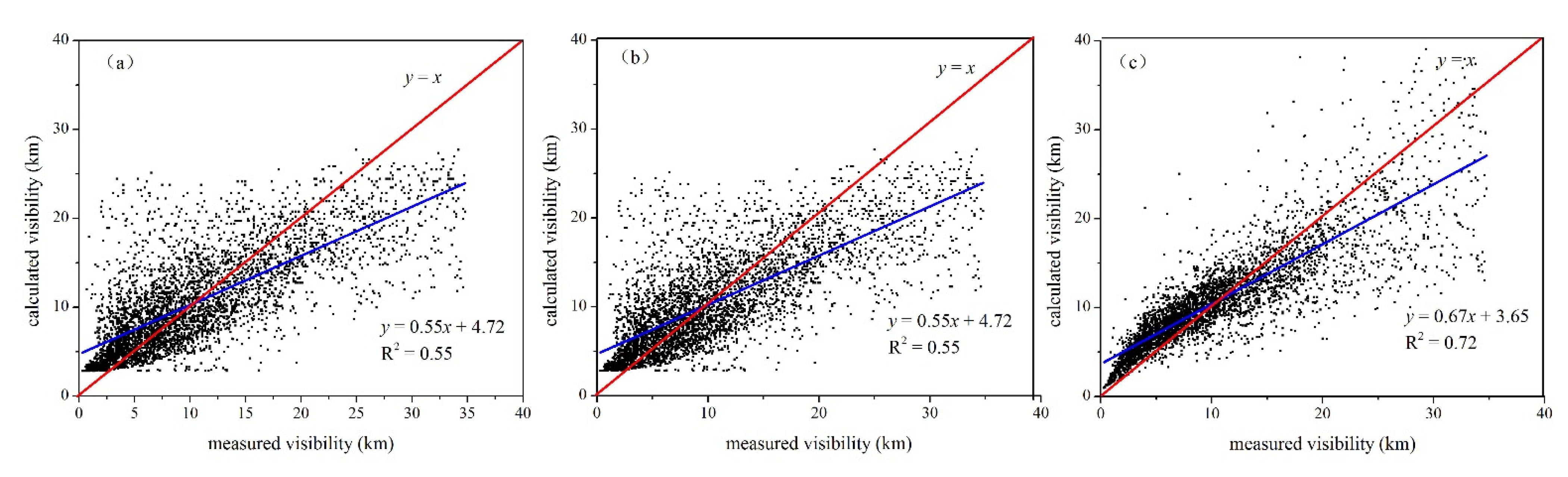
annual	$V=166.1\times {\left[{PM}_{\mathit{2.5}}\right]}^{-0.56}\times {\left(1-RH\right)}^{0.86·RH}$	y = 0.67x + 3.65	0.72

). The calculated visibility for types 1, 2, and 4 fitted the measured visibility less effectively; R² was 0.65, 0.66, and 0.64, respectively. The R² between the measured and calculated visibility in aerosols with high hygroscopic and low non-hygroscopic content (types 3, 5, and 6) was above 0.76. The linear slopes of correlation between calculated and measured visibility were higher (0.72–0.84) in types 3, 5, and 6 than in other types. The fitting equation for types 3, 5, and 6 increased the accuracy of the parameterization scheme for visibility calculation.

Based on the division method of visibility control categories established in Section 2.3, the thresholds for identifying the PM_2.5-sensitive regime and RH-sensitive regime under different aerosol types were determined (Figure 8).

The PM_2.5 and RH thresholds of varied visibility-sensitive regimes differed with aerosol types. When visibility was 10 km, the PM_2.5-sensitive regime was identified by RH < 30%, 31%, 26%, 26%, 25%, and 20% and PM_2.5 > 129, 141, 106, 117, 91, and 146 μg/m³ in types 1–6, respectively. The RH-sensitive regime was characterized by RH > 83%, 85%, 79%, 78%, 78%, and 70% and by PM_2.5 < 40, 45, 26, 30, 22, and 29 μg/m³ in types 1–6, respectively. Other visibility control categories were classified into transition regimes dominated by PM_2.5 and RH with RH = 56%, 58%, 50%, 49%, 49%, and 41% and PM_2.5 = 95, 105, 77, 86, 65, and 103 μg/m³, respectively. The threshold difference of PM_2.5 was by up to 1.6 times.

According to the threshold values of the visibility control categories, the proportion of those in different types in Tianjin, 2015, is shown in

Table 2. Proportion of different visibility-sensitive regimes under varied aerosol types in Tianjin, 2015 (%).

Aerosol Types	PM2.5-Sensitive Regime	Transition Regime Dominated by PM2.5	Transition Regime Dominated by RH	RH-Sensitive Regime
1	27	48	23	2
2	47	47	6	0
3	6	31	59	3
4	9	31	54	6
5	1	13	77	9
6	3	8	46	44
annual	13	31	47	9

. The proportion of transition regimes dominated by PM_2.5 in type 1 was up to 48%, and that of transition regimes dominated by RH was 23%. The proportion of transition regimes dominated by PM_2.5 was still dominant (47%) in type 2. The proportions of the PM_2.5-sensitive regime (47%) in type 2 were higher than those of the other types. The proportions of the transition regimes dominated by PM_2.5 and RH were similar (31% vs. 31% and 59% vs. 54%, respectively) in types 3 and 4. The transition regime dominated by RH became prominent in types 5 and 6 (77% and 46%). The proportions of the RH-sensitive regime were higher than those of other types in type 6 (44%).

4. Conclusions

Many previous studies were performed to explore the complex relationships among visibility, PM_2.5 concentration, and RH. However, the relative contribution of the two factors to visibility degradation, especially for different aerosol types, was difficult to quantify. The impact of chemical compositions on the sensitivity of visibility to PM_2.5 and RH was explored based on the online monitoring data of RH, visibility, PM_2.5, and its major components in this study. The normalized forward sensitivity index method for identifying the dominant factors of visibility was used based on the functional equation among visibility, RH, and PM_2.5 mass concentration given different aerosol types. Visibility was identified as being in the PM_2.5- or RH-sensitive regime according to the corresponding threshold.

The method was verified and evaluated in Tianjin. There was a compound relationship of the power and power-exponential functions among visibility, PM_2.5, and RH. The R² between the calculated and measured visibilities reached 0.72, and the slope was 0.67. Visibility was identified as being in the PM_2.5-sensitive or RH-sensitive regime. Corresponding thresholds of PM_2.5 were determined by function among visibility, PM_2.5, and RH. Chemical compositions ((NH₄)₂SO₄, NH₄NO₃, OC, EC, fine soil, and sea salt) influenced the sensitivity of visibility to PM_2.5 and RH due to varying degrees of dry extinction efficiency and hygroscopicity. A good correlation between visibility and PM_2.5 was found for different aerosol types with the correlation coefficient varying from −0.54 to −0.71. The correlation coefficient between visibility and RH changed from −0.16 to −0.70 with the increase of the content of hygroscopic components. The results showed that the normalized forward sensitivity index method is suitable for various aerosol types and can be applied to identify the leading factors of atmospheric visibility decline as long as synchronous, high-resolution data of visibility, PM_2.5, and RH are collected. However, for different aerosol types, the PM_2.5 thresholds under the same visibility-sensitive regimes can be several times different, while the RH threshold changes gently. The thresholds for different aerosol types obtained in this study can be used as a reference for other cities with the data of extinction component content in PM_2.5. Next, we will further evaluate the applicability of the method in other cities.

References

- Watson, J.G. Critical review discussion-visibility, Science and regulation. J. Air Waste Manag. Assoc. 2002, 52, 973–999. [Google Scholar] [CrossRef] [Green Version]
- Doyle, M.; Dorling, S. Visibility trends in the UK 1950–1997. Atmos. Environ. 2002, 36, 3161–3172. [Google Scholar] [CrossRef]
- Hu, Y.; Yao, L.; Cheng, Z.; Wang, Y. Long-term atmospheric visibility trends in megacities of China, India and the United States. Environ. Res. 2017, 159, 466–473. [Google Scholar] [CrossRef] [PubMed]
- Li, J.; Li, C.; Zhao, C.; Su, T. Changes in surface aerosol extinction trends over China during 1980–2013 inferred from quality-controlled visibility data. Geophys. Res. Lett. 2016, 43, 8713–8719. [Google Scholar] [CrossRef] [Green Version]
- Zhang, F.; Xu, L.; Chen, J.; Yu, Y.; Niu, Z.; Yin, L. Chemical compositions and extinction coefficients of PM2.5 in peri-urban of Xiamen, China, during June 2009–May 2010. Atmos. Res. 2012, 106, 150–158. [Google Scholar] [CrossRef]
- Founda, D.; Kazadzis, S.; Mihalopoulos, N.; Gerasopoulos, E.; Lianou, M.; Raptis, P.I. Long-term visibility variation in Athens (1931–2013): A proxy for local and regional atmospheric aerosol loads. Atmos. Chem. Phys. 2016, 16, 11219–11236. [Google Scholar] [CrossRef] [Green Version]
- Han, L.; Sun, Z.; He, J.; Hao, Y.; Tang, Q.; Zhang, X.; Zheng, C.; Miao, S. Seasonal variation in health impacts associated with visibility in Beijing, China. Sci. Total Environ. 2020, 730, 139149. [Google Scholar] [CrossRef]
- Singh, A.; Dey, S. Influence of aerosol composition on visibility in megacity Delhi. Atmos. Environ. 2012, 62, 367–373. [Google Scholar] [CrossRef]
- Shen, X.; Sun, J.; Zhang, X.; Zhang, Y.; Zhang, L.; Che, H.; Ma, Q.; Yu, X.; Yue, Y. Characterization of submicron aerosols and effect on visibility during a severe haze-fog episode in Yangtze River Delta, China. Atmos. Environ. 2015, 120, 307–316. [Google Scholar] [CrossRef] [Green Version]
- Singh, A.; Bloss, W.J.; Pope, F.D. 60 years of UK visibility measurements: Impact of meteorology and atmospheric pollutants on visibility. Atmos. Chem. Phys. 2017, 17, 2085–2101. [Google Scholar] [CrossRef] [Green Version]
- Cao, J.-J.; Wang, Q.-Y.; Chow, J.C.; Watson, J.; Tie, X.-X.; Shen, Z.-X.; Wang, P.; An, Z.-S. Impacts of aerosol compositions on visibility impairment in Xi’an, China. Atmos. Environ. 2012, 59, 559–566. [Google Scholar] [CrossRef]
- Shen, Z.X.; Cao, J.J.; Arimoto, R.; Han, Z.; Zhang, R.; Han, Y.; Liu, S.; Okuda, T.; Nakao, S.; Tanaka, S. Ionic composition of TSP and PM2.5 during dust storms and air pollution episodes at Xi’an, China. Atmos. Environ. 2009, 43, 2911–2918. [Google Scholar] [CrossRef]
- Wang, H.; Xu, J.; Zhang, M.; Yang, Y.; Shen, X.; Wang, Y.; Chen, D.; Guo, J. A study of the meteorological causes of a prolonged and severe haze episode in January 2013 over central-eastern China. Atmos. Environ. 2014, 98, 146–157. [Google Scholar] [CrossRef]
- Zhang, Q.; Quan, J.N.; Tie, X.X.; Li, X.; Liu, Q.; Gao, Y.; Zhao, D.L. Effects of meteorology and secondary particle formation on visibility during heavy haze events in Beijing, China. Sci. Total Environ. 2015, 502, 578–584. [Google Scholar] [CrossRef] [PubMed]
- Luan, T.; Guo, X.L.; Guo, L.J.; Zhang, T. Quantifying the relationship between PM2.5 concentration, visibility and planetary boundary layer height for long-lasting haze and fog-haze mixed events in Beijing. Atmos. Chem. Phys. 2018, 18, 203–225. [Google Scholar] [CrossRef] [Green Version]
- Zhao, P.; Zhang, X.; Xu, X.; Zhao, X. Long-term visibility trends and characteristics in the region of Beijing, Tianjin, and Hebei, China. Atmos. Res. 2011, 101, 711–718. [Google Scholar] [CrossRef]
- Huang, K.; Zhuang, G.; Lin, Y.; Wang, Q.; Fu, J.S.; Zhang, R.; Li, J.; Deng, C.; Fu, Q. Impact of anthropogenic emission on air quality over a megacity-revealed from an intensive atmospheric campaign during the Chinese Spring Festival. Atmos. Chem. Phys. 2012, 12, 11631–11645. [Google Scholar] [CrossRef] [Green Version]
- Kong, L.; Xin, J.; Liu, Z.; Zhang, K.; Tang, G.; Zhang, W.; Wang, Y. The PM2.5 threshold for aerosol extinction in the Beijing megacity. Atmos. Environ. 2017, 167, 458–465. [Google Scholar] [CrossRef]
- Wang, X.; Zhang, R.; Yu, W. The Effects of PM2.5 Concentrations and Relative Humidity on Atmospheric Visibility in Beijing. J. Geophys. Res. Atmos. 2019, 124, 2235–2259. [Google Scholar] [CrossRef]
- Deng, H.; Tan, H.; Li, F.; Cai, M.; Chan, P.W.; Xu, H.; Huang, X.; Wu, D. Impact of relative humidity on visibility degradation during a haze event: A case study. Sci. Total Environ. 2016, 569–570, 1149–1158. [Google Scholar] [CrossRef]
- Malm, W.C.; Day, D.E. Estimates of aerosol species scattering characteristics as a function of relative humidity. Atmos. Environ. 2001, 35, 2845–2860. [Google Scholar] [CrossRef]
- Chen, J.; Zhao, C.S.; Ma, N.; Liu, P.F.; Göbel, T.; Hallbauer, E.; Deng, Z.Z.; Ran, L.; Xu, W.Y.; Liang, Z.; et al. A parameterization of low visibilities for hazy days in the North China Plain. Atmos. Chem. Phys. 2012, 12, 4935–4950. [Google Scholar] [CrossRef] [Green Version]
- Wu, Y.; Wang, X.; Yan, P.; Zhang, L.; Tao, J.; Liu, X.; Tian, P.; Han, Z.; Zhang, R. Investigation of hygroscopic growth effect on aerosol scattering coefficient at a rural site in the southern North China Plain. Sci. Total Environ. 2017, 599–600, 76–84. [Google Scholar] [CrossRef]
- Covert, D.S.; Charlson, R.J.; Ahlquist, N.C. A Study of the Relationship of Chemical Composition and Humidity to Light Scattering by Aerosols. J. Appl. Meteorol. 1972, 11, 968–976. [Google Scholar] [CrossRef] [Green Version]
- Li, Y.; Huang, H.X.; Griffith, S.M.; Wu, C.; Lau, A.K.; Yu, J.Z. Quantifying the relationship between visibility degradation and PM2.5 constituents at a suburban site in Hong Kong: Differentiating contributions from hydrophilic and hydrophobic organic compounds. Sci. Total Environ. 2017, 575, 1571–1581. [Google Scholar] [CrossRef] [PubMed]
- Wen, C.-C.; Yeh, H.-H. Comparative influences of airborne pollutants and meteorological parameters on atmospheric visibility and turbidity. Atmos. Res. 2010, 96, 496–509. [Google Scholar] [CrossRef]
- Schichtel, B.A.; Husar, R.B.; Falke, S.R.; Wilson, W.E. Haze trends over the United States, 1980–1995. Atmos. Environ. 2001, 35, 5205–5210. [Google Scholar] [CrossRef]
- Sun, Y.; Chen, C.; Zhang, Y.; Xu, W.; Zhou, L.; Cheng, X.; Zheng, H.; Ji, D.; Li, J.; Tang, X.; et al. Rapid formation and evolution of an extreme haze episode in Northern China during winter 2015. Sci. Rep. 2016, 6, 27151. [Google Scholar] [CrossRef] [PubMed] [Green Version]
- Day, D.E.; Malm, W.C. Aerosol light scattering measurements as a function of relative humidity: A comparison between measurements made at three different sites. Atmos. Environ. 2001, 35, 5169–5176. [Google Scholar] [CrossRef]
- Wang, B.; Chen, Y.; Zhou, S.; Li, H.; Wang, F.; Yang, T. The influence of terrestrial transport on visibility and aerosol properties over the coastal East China Sea. Sci. Total Environ. 2018, 649, 652–660. [Google Scholar] [CrossRef] [PubMed]
- Tao, J.; Zhang, L.; Engling, G.; Zhang, R.; Yang, Y.; Cao, J.; Zhu, C.; Wang, Q.; Luo, L. Chemical composition of PM2.5 in an urban environment in Chengdu, China: Importance of springtime dust storms and biomass burning. Atmos. Res. 2012, 122, 270–283. [Google Scholar] [CrossRef]
- Ye, B.M.; Ji, X.L.; Yang, H.Z.; Yao, X.; Chan, K.C.; Cadle, S.H.; Chan, T.; Mulawa, P.A. Concentration and chemical composition of PM2.5 in Shanghai for a 1-year period. Atmos. Environ. 2003, 37, 499–510. [Google Scholar] [CrossRef]
- Ma, N.; Zhao, C.; Chen, J.; Xu, W.; Yan, P.; Zhou, X. A novel method for distinguishing fog and haze based on PM2.5, visibility, and relative humidity. Sci. China Earth Sci. 2014, 57, 2156–2164. [Google Scholar] [CrossRef]
- Liu, B.; Yang, J.; Yuan, J.; Wang, J.; Dai, Q.; Li, T.; Bi, X.; Feng, Y.; Xiao, Z.; Zhang, Y.; et al. Source apportionment of atmospheric pollutants based on the online data by using PMF and ME2 models at a megacity, China. Atmos. Res. 2017, 185, 22–31. [Google Scholar] [CrossRef]
- Li, Y.F.; Liu, B.S.; Xue, Z.G.; Zhang, Y.F. Chemical characteristics and source apportionment of PM2.5 using PMF modelling coupled with 1-h resolution online air pollutant dataset for Linfen, China. Environ. Pollut. 2020, 263, 114532. [Google Scholar] [CrossRef]
- Song, M.; Han, S.Q.; Zhang, M.; Yao, Q.; Zhu, B. Relationship between visibility and relative humidity, PM10, PM2.5 in Tianjin. J. Meteor. Environ. 2013, 29, 34–41. (In Chinese) [Google Scholar]
- Randriamiarisoa, H.; Chazette, P.; Couvert, P.; Sanak, J.; Mégie, G. Relative humidity impact on aerosol parameters in a Paris suburban area. Atmos. Chem. Phys. 2006, 6, 1389–1407. [Google Scholar] [CrossRef] [Green Version]
- Carrico, C.M.; Rood, M.J.; Ogren, J.A.; Neusüss, C.; Wiedensohler, A.; Heintzenberg, J.; Neusüß, C. Aerosol Optical properties at Sagres, Portugal during ACE-2. Tellus B Chem. Phys. Meteorol. 2000, 52, 694–715. [Google Scholar] [CrossRef]
- Chitnis, N.; Hyman, J.; Cushing, J. Determining Important Parameters in the Spread of Malaria through the Sensitivity Analysis of a Mathematical Model. Bull. Math. Biol. 2008, 70, 1272–1296. [Google Scholar] [CrossRef] [PubMed]
- Aguilar-Canto, F.J.; de León, U.A.-P.; Avila-Vales, E. Sensitivity theorems of a model of multiple imperfect vaccines for COVID-19. Chaos Solitons Fractals 2022, 156, 111844. [Google Scholar] [CrossRef] [PubMed]
- Malm, W.C.; Gebhart, K.A.; Molenar, J.; Cahill, T.; Eldred, R.; Huffman, D. Examining the relationship between atmospheric aerosols and light extinction at Mount-Rainier-National-Park and North-Cascades-National-Park. Atmos. Environ. 1994, 28, 347–360. [Google Scholar] [CrossRef]
- Pitchford, M.; Malm, W.; Schichtel, B.; Kumar, N.; Lowenthal, D.; Hand, J. Revised algorithm for estimating light extinction from IMPROVE particle speciation data. J. Air Waste Manag. Assoc. 2007, 57, 1326–1336. [Google Scholar] [CrossRef] [PubMed]
- Wang, J.; Zhang, Y.-F.; Feng, Y.-C.; Zheng, X.-J.; Jiao, L.; Hong, S.-M.; Shen, J.-D.; Zhu, T.; Ding, J.; Zhang, Q. Characterization and source apportionment of aerosol light extinction with a coupled model of CMB-IMPROVE in Hangzhou, Yangtze River Delta of China. Atmos. Res. 2016, 178–179, 570–579. [Google Scholar] [CrossRef]
- Wang, Q.; Sun, Y.; Jiang, Q.; Du, W.; Sun, C.; Fu, P.; Wang, Z. Chemical composition of aerosol particles and light extinction apportionment before and during the heating season in Beijing, China. J. Geophys. Res. Atmos. 2015, 120, 12708–12722. [Google Scholar] [CrossRef]
- Turpin, B.J.; Lim, H.J. Species Contributions to PM2.5 Mass Concentrations: Revisiting Common Assumptions for Estimating Organic Mass. Aerosol. Sci. Technol. 2001, 35, 602–610. [Google Scholar] [CrossRef]
- Zou, J.; Liu, Z.; Hu, B.; Huang, X.; Wen, T.; Ji, D.; Liu, J.; Yang, Y.; Yao, Q.; Wang, Y. Aerosol chemical compositions in the North China Plain and the impact on the visibility in Beijing and Tianjin. Atmos. Res. 2018, 201, 235–246. [Google Scholar] [CrossRef]
- Tao, J.; Zhang, L.; Gao, J.; Wang, H.; Chai, F.; Wang, S. Aerosol chemical composition and light scattering during a winter season in Beijing. Atmos. Environ. 2015, 110, 36–44. [Google Scholar] [CrossRef]
- Aldabe, J.; Elustondo, D.; Santamaría, C.; Lasheras, E.; Pandolfi, M.; Alastuey, A.; Querol, X.; Santamaría, J.M. Chemical characterisation and source apportionment of PM2.5 and PM10 at rural, urban and traffic sites in Navarra (North of Spain). Atmos. Res. 2011, 102, 191–205. [Google Scholar] [CrossRef]
- Fu, X.; Wang, X.; Hu, Q.; Li, G.; Ding, X.; Zhang, Y.; He, Q.; Liu, T.; Zhang, Z.; Yu, Q.; et al. Changes in visibility with PM2.5 composition and relative humidity at a background site in the Pearl River Delta region. J. Environ. Sci. 2016, 40, 10–19. [Google Scholar] [CrossRef] [PubMed]
- Yu, X.; Ma, J.; An, J.; Yuan, L.; Zhu, B.; Liu, D.; Wang, J.; Yang, Y.; Cui, H. Impacts of meteorological condition and aerosol chemical compositions on visibility impairment in Nanjing, China. J. Clean. Prod. 2016, 131, 112–120. [Google Scholar] [CrossRef]