Article

The Trend and Interannual Variability of Marine Heatwaves over the Bay of Bengal

1
Key Laboratory of Marine Hazards Forecasting, Ministry of Natural Resources, Hohai University, Nanjing 210098, China
2
College of Oceanography, Hohai University, Nanjing 210098, China
3
Southern Marine Science and Engineering Laboratory (Zhuhai), Zhuhai 519082, China
4
Information Center, Ministry of Water Resources of China, Beijing 100053, China
*
Author to whom correspondence should be addressed.
Atmosphere 2022, 13(3), 469; https://doi.org/10.3390/atmos13030469
Submission received: 10 February 2022 / Revised: 9 March 2022 / Accepted: 10 March 2022 / Published: 14 March 2022
(This article belongs to the Special Issue Tropical Ocean-Atmosphere Interaction and Climate Change)

Abstract

:
Marine heatwaves (MHWs) are long-lasting extreme oceanic warming events that can cause devastating effects on warm-water corals and associated ecosystems. The linear trend and interannual variability of MHWs over the Bay of Bengal (BOB) during 1982–2020 are investigated by a high-resolution daily sea surface temperature (SST) dataset. In regions where warm-water coral reefs are concentrated, annual MHW days and frequency significantly increase during 1982–2020, at rates exceeding that of the global mean. The coldest boreal winter season witnesses significant and steady increase trends in MHW days and frequency. In contrast, the trend is insignificant in the climatological warmest season (March to June) south of 15° N in the BOB, mainly due to large interannual variability. El Niño and Southern Oscillation (ENSO) dominates the interannual variability of BOB MHWs, which are highly consistent with the evolution of the mean SST. The negative phase of North Atlantic Oscillation (NAO) also modulates the occurrences of MHWs, especially over the northeastern BOB. The two climate modes synergistically explain about 50~70% of the interannual variances in the BOB’s MHWs. Correlation analysis reveals that south of 15° N in the BOB, the effect of El Niño on MHWs is evident from the boreal autumn of its developing phase to the boreal summer of its decaying phase, along with limited influence from NAO. However, in the northeast of the BOB, the effect of El Niño merely emerges from April to August of its decaying stage. In comparison, boreal winter-to-spring NAO exerts a strong control over March-to-June MHWs in the northeastern BOB. The results suggest that various climate modes may jointly or separately influence MHWs at certain seasons and locations, which is important for the seasonal prediction of MHWs. Indeed, when combining the Niño3.4 mature winter index and boreal winter-to-spring NAO index to build a regression model, it is more effective in reproducing the BOB’s MHW frequency compared to the Niño3.4 index alone.

1. Introduction

Marine heatwaves (MHWs) are extreme sea surface temperature (SST) warming events lasting for several days, weeks or even months. The resultant coral bleaching, seagrass meadow destruction and species migration are devastating for marine ecosystems and fishery production [1,2,3,4]. However, MHWs receive great attention only after the 2011 West Australian MHW, despite their devastating effects [5,6]. Under global warming, MHWs are projected to occur more frequently with prolonged days [7,8,9], further damaging or even destroying the living conditions of marine life. This highlights the importance of investigating the drivers and mechanisms of MHWs, and hence improving the short-term predictions and long-term projections [10,11,12].
Previous studies mostly focus on the mechanisms of MHWs in a few hot regions or discuss the mechanisms on a global scale. The mechanisms of individual MHW cases display large differences across regions, but mainly relate to local oceanic and atmospheric conditions, air–sea coupling and climate mode-associated remote teleconnections [6,13,14,15]. For example, the anomalous air–sea heat flux generated by the atmospheric high-pressure system lead to the 2003 Mediterranean MHW [16], and abnormal ocean advection causes the 2015/16 Tasman Sea MHW [17] and the southeastern tropical Indian Ocean MHW [18]. Climate modes play an important role in modulating the variability of MHWs, but the dominant modes substantially vary across regions. Generally, MHWs are closely associated with the El Niño and Southern Oscillation (ENSO), the Indian Ocean basin mode (IOB) and dipole mode (IOD) and the Pacific Decadal Oscillation (PDO) in Indo-Pacific regions [19,20,21,22,23,24,25,26]. The North Atlantic Oscillation (NAO) is also shown to be connected with the formation of Indian Ocean MHWs [13,24].
The Bay of Bengal (BOB) is a critical region of the Indian Ocean because it supports large marine primary productivity and is strongly coupled with the Indian monsoon [27]. Additionally, the BOB suffers powerful and deadly tropical cyclones as it supplies warm SSTs and high humidity year-around. Additional extreme and prolonged warming beyond the high SSTs can cause severe disasters in marine ecosystems, such as the 2010 Andaman sea MHW [28], and may even regulate the Indian summer monsoon [24] and cyclone activities. However, the BOB MHWs during the last decades have lacked systematic and in-depth investigations, with their evolution features in recent decades remaining unclear. For example, El Niño is revealed to have caused two peak warming in the North Indian Ocean during its developing phase and decaying phase, respectively [29,30,31]. Therefore, the BOB MHWs may also be more active during the North Indian Ocean peak warming periods. The detailed relationship between the BOB and climate modes has not yet been systematically revealed. Global warming is supposed to cause an increasing trend in the duration and frequency of MHWs over most oceans [13,15]. Given that the warming trend is predicted to continue in the near future, background condition changes may further fuel the BOB MHWs when favorable climate modes occur.
Therefore, the present study investigates the linear trend and interannual variability of BOB MHWs during 1982–2020, when satellite observation data was widely available. We show that the BOB’s annual MHW days and frequency significantly increase at rates that are larger than that of the global mean. Causality analysis shows that the increasing trends of BOB MHWs are clearly driven by the rise in atmospheric CO2 concentration. However, the linear trend is not significant in the warmest season, especially for boreal spring. The interannual variability of BOB MHWs is large and mainly dominated by ENSO, with the negative phase of the boreal winter-to-spring NAO also being effective in regulating their occurrences, especially over the northeastern BOB. The two climate modes synergistically explain about 50~70% of the interannual variances in the BOB MHWs.
The rest of this paper is organized as follows: Section 2 describes the definition of MHWs, data and methods; Section 3 shows the climatology and linear trend of the BOB MHWs’ properties; Section 4 investigates the interannual variability of the BOB MHWs and underlying processes; and Section 5 presents the discussion and summary.

2. Data and Methods

2.1. Data

Coral reef data (WCMC008 v4.1) shown in Figure 1a is collected from 1954–2018 by the UNEP World Conservation Monitoring Centre (UNEP-WCMC) and the WorldFish Centre, in collaboration with the WRI (World Resources Institute) and TNC (The Nature Conservancy). Data sources include the Millennium Coral Reef Mapping Project [32,33] and the World Atlas of Coral Reefs [34]. It shows coral reef distributions in the tropical and subtropical regions and is the most comprehensive empirical global dataset of warm-water coral reefs to date. The high-resolution daily SST analysis (Optimum Interpolation SST, OISST) are developed using the optimum interpolation method [35]. The analyses have a spatial grid resolution of 0.25° and a temporal resolution of 1 day, and the cold bias against Argo is about −0.14 °C on a global average and −0.28 °C in the Indian Ocean during 2016–2019. It is the most used dataset for the detection of MHWs. We also utilized it to detect MHWs from January 1982 to December 2020 in the BOB. Atmospheric carbon dioxide measured at Mauna Loa provides the longest record of atmospheric CO2 concentrations [36,37]. The monthly mean NAO index, since 1950, is provided by the National Weather Service Climate Prediction Center.

2.2. MHW Definition

Following Hobday et al. (2016), an MHW is defined as a prolonged discrete anomalously warm-water event in which SST warming exceeds a threshold of the 90th percentile based on the climatological daily mean and lasts for at least 5 days. The 90th percentile and climatology are calculated within an 11-day window centered on each calendar day, and then smoothed in a 31-day running mean window by the daily SST from 1982 to 2020 [14,38,39]. By this definition, MHWs can be identified at any time of the year, including the local winter season. An MHW is primarily measured by the metrics of its days (MHW days, number of days between the specific period), frequency (MHW frequency, number of MHWs during a specific period) and mean intensity (MHW intensity, averaged SST anomaly during each MHW event). In this study, MHW days and frequency are attributed to be zero when no MHW occurs during a certain period.

2.3. Causality Analysis

Following Liang (2014) [40], the causality between two time series ( X 1 and X 2 ) can be judged by the Liang–Kleeman information flow theory. The exchange of information between two events indicates the quantity as well as the direction of the causality. Liang (2014, 2015, 2016) [40,41,42] show that if the development of X 1 is independent of X 2 , then there is zero information flow from X 2 to X 1 . For the linear systems, the maximum likelihood estimator of it can be estimated as:
T 2 1 = C 11 C 12 C 2 , d 1 C 12 2 C 1 , d 1 C 11 2 C 22 C 11 C 12 2 .                          
where C i j is the sample covariance between X i and X j , C i , d j is the sample covariance between X i and X j , which is defined as X j = X j , n + 1 X j , n Δ t , and Δ t is the time step. If T 2 1 = 0 , X 2 does not cause X 1 ; if T 2 1 0 and the value passes the statistical significance test, X 2 is deemed to cause X 1 [40,41,42]. Stips et al. (2016) suggest that if T 2 1   T 1 2 , X 2 is also supposed to cause X 1 ; if they are comparable and both pass the significance test, there is a reciprocal causation. The calculation script of the method is available at http://www.ncoads.cn/article/show/63.aspx, accessed on 8 March 2022. This method has been widely applied in different studies to explore the causality between different time series [43,44,45,46,47].

2.4. Study Area

The devastating nature of extreme warming on coral polyps results in warm-water coral reefs being increasingly threatened by MHWs. Warm-water coral reefs are highly restricted in areas of warm, shallow and clear water to produce the copious quantities of limestone necessary for reef formation. To focus on the influence of MHWs on coral bleaching, we selected three regions in which coral reefs are concentrated, that is Region 1 (77°–83° E, 5° N–12.5° N) around Sri Lanka, Region 2 (91°–100° E, 5° N–14° N) in the Andaman Sea and Region 3 (91°–95° E, 15.5° N–21° N) in the northeast of the BOB.

3. Climatology and Linear Trend of the BOB MHWs

3.1. MHWs Climatology

Figure 1 displays the warm-water coral reef distribution and climatology of MHWs’ annual days, frequency and mean intensity over the BOB for 1982–2020. In the Andaman Sea, where most coral reefs are located, MHWs take place more than 22 days per year in climatology (Figure 1b). North of 15° N or east of 90° E, MHWs display relatively more days and exhibit a larger intensity than those in the western and southern regions of the BOB in climatology (Figure 1b,d). For the frequency (Figure 1c), MHWs occur around 2 times/year in most regions and display weak spatial variations. To illustrate the influence of MHWs on warm-water coral reefs, three regions were selected as the focus of this study (black box in Figure 1a), with Region 1 (77°–83° E, 5° N–12.5° N) in the southwest of the BOB, Region 2 (91°–100° E, 5° N–14° N) in the Andaman Sea and Region 3 (91°–95° E, 15.5° N–21° N) in the northeastern BOB. Region 1 displays much fewer MHW days (below 20 days per year) than the other two regions. Ocean temperature varies seasonally following the migration of the subsolar point. In climatology, Regions 1 and 2 generally experience high SSTs above 28.5 °C from boreal spring to autumn (Figure 1e–g), with the highest SST appearing during boreal spring. The SST in Region 3 displays two distinct peaks in May and October, respectively, and is above 28.5 °C from April to November.

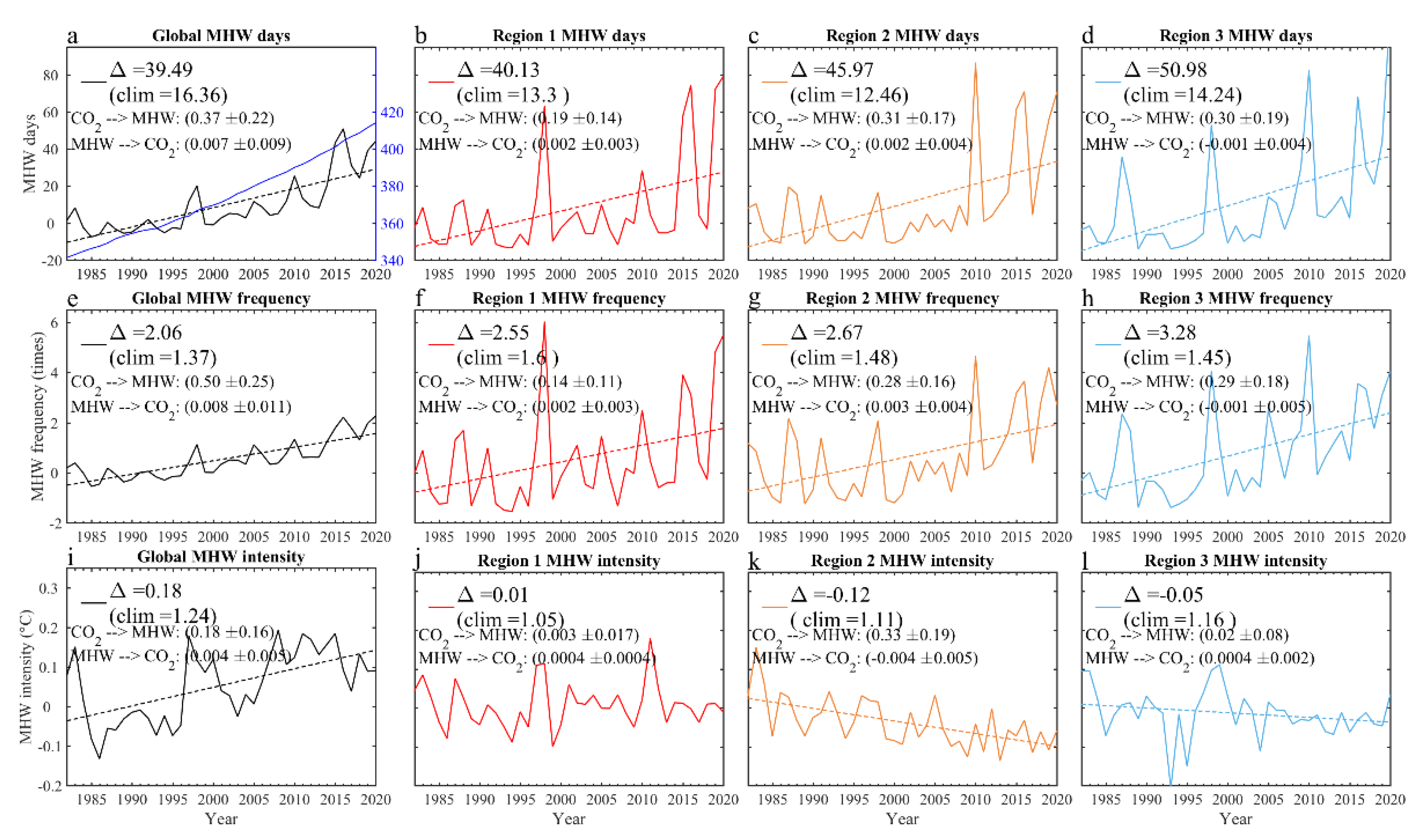
3.2. Linear Trend of the BOB MHWs

We respectively calculated the area-weighted-mean MHW days, frequency and intensity of global oceans, Region 1, Region 2 and Region 3 (Figure 2). The global mean annual MHW days display a trend of about 1.01 days/year during 1982–2020, i.e., a total change of 39.49 days in the 39-year period, which is more than 2 times of the 1982–2000 mean value. Compared to the global mean, the annual MHW days show a relatively larger trend of 1.03 days/year, 1.18 days/year and 1.31 days/year in Region 1, Region 2 and Region 3, respectively. The total increase in the annual MHW days in all three regions are more than three times of the 1982–2000 value, exceeding that of global oceans. For the occurrence, annual MHWs take place about 1.37 times for global oceans and about 1.45~1.6 times for the 1982–2000 mean in the three regions. The MHW frequency displays a trend that is weaker and insignificant (larger and significant) than the global oceans in Region 1, Region 2 and Region 3. Generally, MHWs display trends in days and frequencies that are larger in all three regions (exceeding 0.065 times/year) than global oceans (0.05 times/year). Causality analysis reveals that there is a significant information flow from the atmospheric CO2 concentration (Figure 1a blue line) to MHW days. In contrast, the information flow from MHW days to CO2 is negligible and insignificant. The results are similar for the information flow analysis between MHW frequency and CO2. Moreover, for the linear trends of MHW intensity that are not significant or negligible (Region 1 and Region 2), the values of the two-way information flow both fail to pass the significance test (Figure 2j,l). This also confirms the effectiveness of the information flow analysis in revealing the causality. Therefore, the significant increase trends in MHWs are clearly caused by the increase in atmospheric CO2 concentrations (Figure 1a blue line). However, MHW intensity is above 1 °C in climatology and displays insignificant or even weak negative trends in three regions (Figure 2j–l), contrasting with the slightly increased global mean MHW intensity (Figure 2i). By definition, MHWs are extreme oceanic warming events with large intensity of SST anomalies. MHW intensity is calculated as the mean SST anomalies relative to the climatological daily mean of all the MHWs during specific time intervals, indicating that MHW intensity may also be high during early periods. As MHWs become more frequent and prolonged, the extended MHW days may decrease the averaged intensity of temperature anomalies for MHWs, causing negative trends in the MHW intensity in Region 2 despite the SST increase.
Furthermore, Figure 3 shows the spatial pattern of the estimated total change during the 39-year period (1982–2020), based on the linear trend coefficients in annual mean SSTs, and annual MHW days and frequencies in the BOB. The SST displays basin-wide warming in the BOB (Figure 3a), with a linear trend above 0.4 °C in most regions. Specifically, the warming is slightly high in Region 3 (above 0.5 °C), while it is low in Region 1 (below 0.4 °C). In comparison, there are relatively larger spatial variations in the trends of MHW days and frequencies than the annual mean SST (Figure 3b,c). Annual MHW days significantly increase east of 85° E, with a trend of above 1.03 days/year, i.e., a total change of 40 days during 1982–2020 that is about 2 times of the 1982–2000 mean value. The MHW frequency significantly increases in Region 3 and south of 12° N in Region 2, but displays an insignificant trend in Region 1. These results indicate that warm-water coral reefs suffer from larger increases in MHW days and frequency in the east and north of the BOB than the west, during 1982–2020.
Warm-water reef-building corals need a steady water temperature of 18 °C to 30 °C to live and grow; a surge of 1–2 °C warming above the upper limit of this livable range and sustained over weeks can cause devastating effects on corals. Therefore, coral reefs may be more vulnerable to MHWs occurring at seasons with a background high SST; we further calculated the area-weighted mean MHW frequency in the three regions during boreal winter (December–January–February, DJF), spring (March–April–May, MAM), summer (June–July–August, JJA) and autumn (September–October–November– SON) during 1982–2020 (Figure 4).
MHW frequency increases significantly in all three regions in DJF, when the seasonal SST (Figure 1e–g) and MHW frequency (Figure 4a–c) are both the lowest. The total change of MHW frequency during 1982–2020 is more than 2 times of the 1982–2000 mean value. In MAM, the trends are not prominent in Region 1 and Region 2, but significant in Region 3 when the seasonal SST and climatological MHW frequency are the highest. In JJA, significant trends only appear in Region 1 and Region 3 (Figure 4g,i) and are comparable with the 1920–2000 climatology in magnitude. In Region 3, the trend of the MHW frequency is insignificant in SON when the seasonal SST is also high (Figure 4l), in contrast to the prominent trends during SON in Region 1 and Region 2. These results indicate that the effect of global warming on warm season MHWs is still weaker than the natural variability over the BOB, especially south of 15° N. Further examination is needed on MHWs’ variability, especially at interannual time scale.

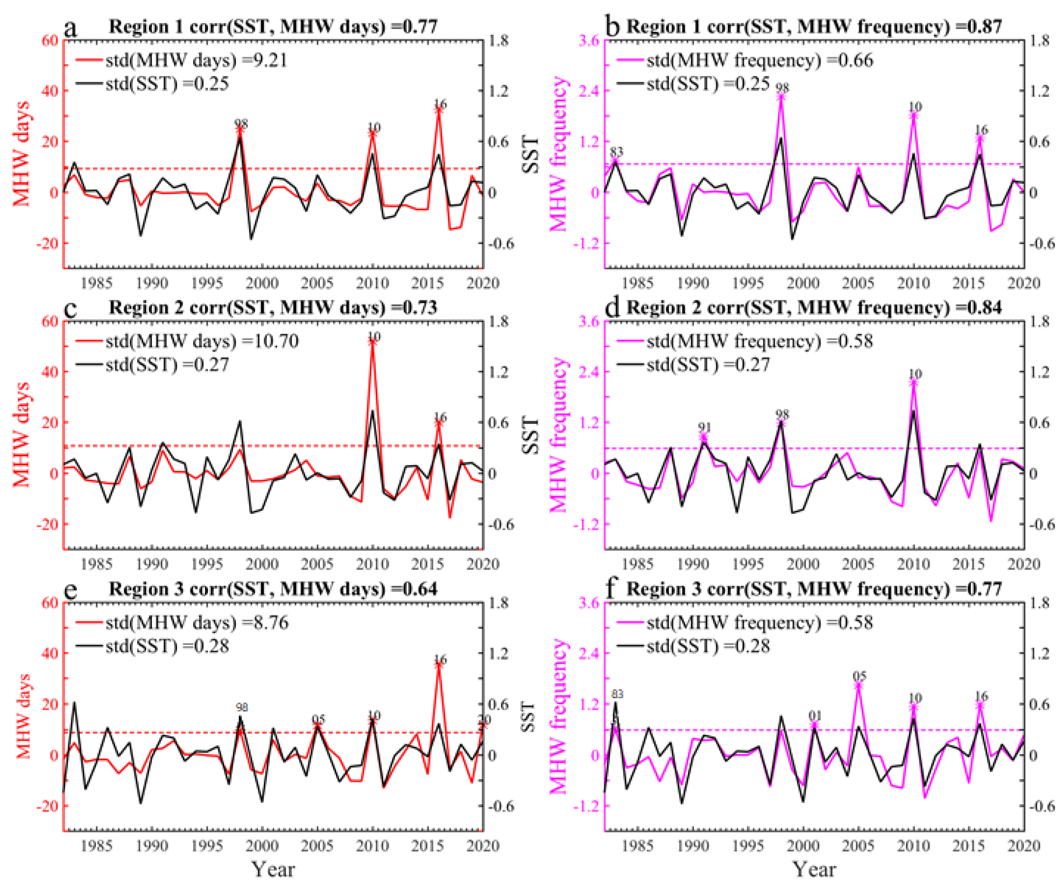
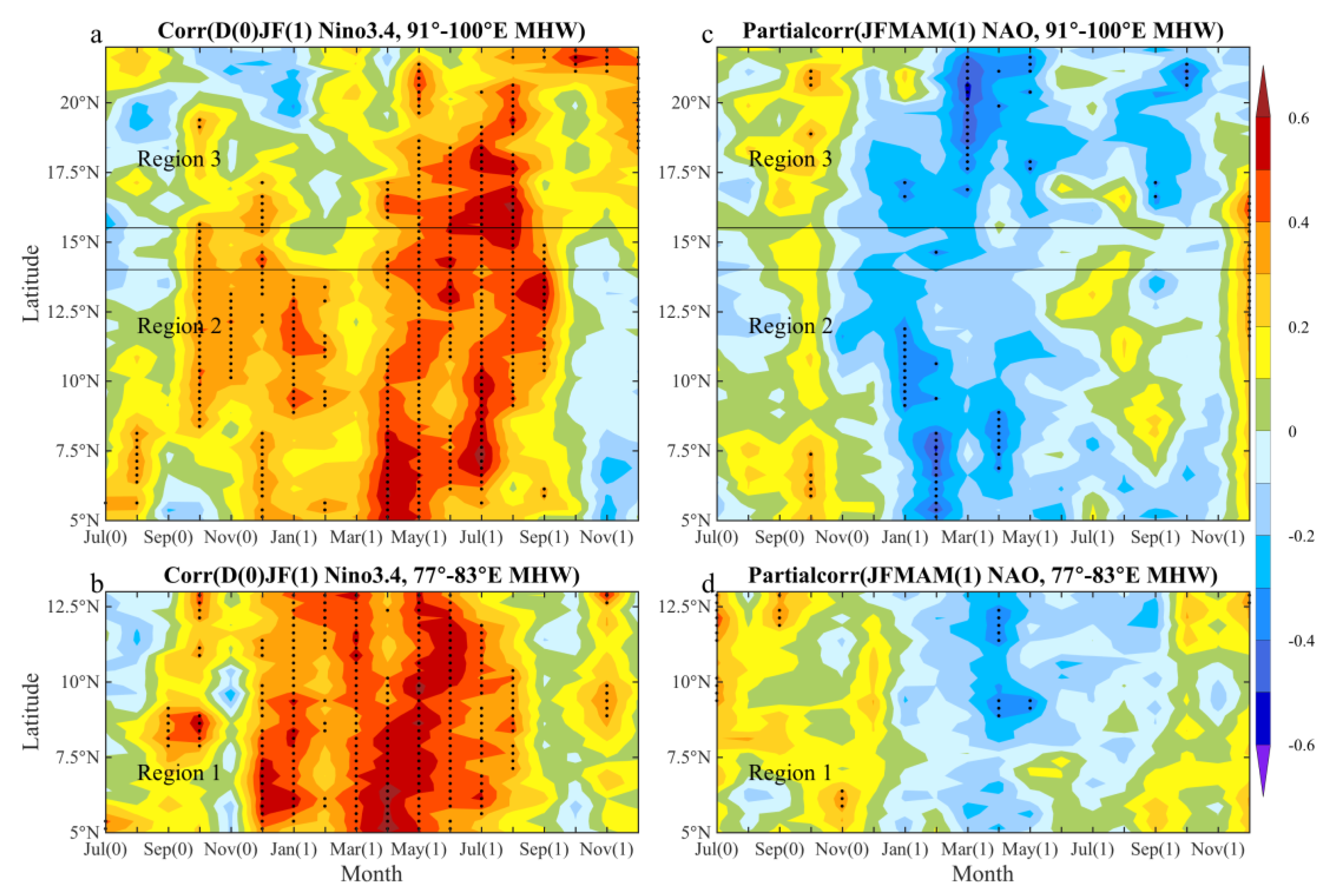
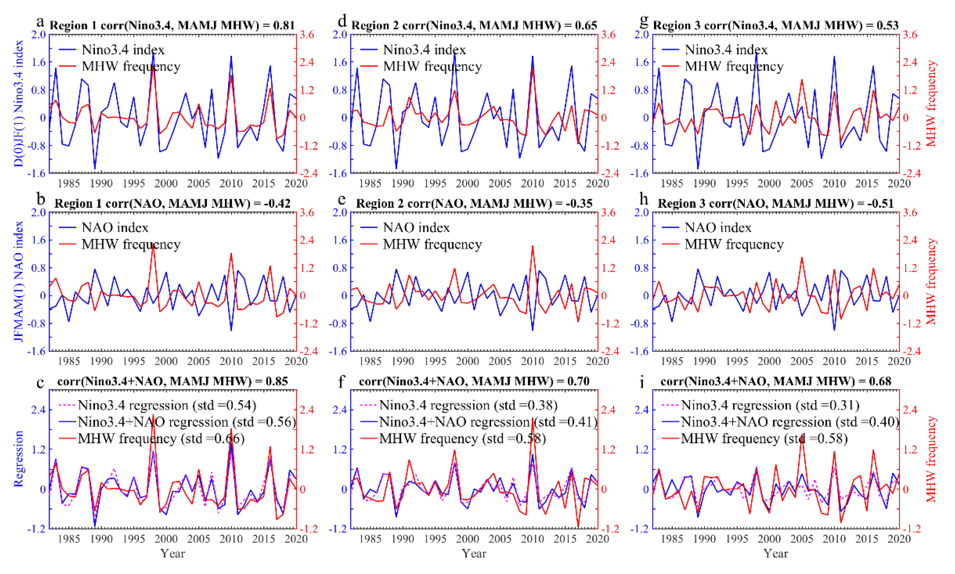
4. Interannual Variability of the BOB MHWs

To investigate the interannual variability in warm season MHWs, a 7-year high-pass filter is applied to the detrended time series of the March–April–May–June (MAMJ) mean SST and MHW days and frequency in the three regions (Figure 5). Here, the warmest boreal spring season is selected to highlight the effectiveness of extreme warm water on coral reef bleaching. Indeed, the variations in the MHW days and frequency are highly consistent with the local SST variability at an interannual time scale, with significant correlation coefficients between the local SST and MHW days (frequency) above 0.73 (0.84) in Region 1 and Region 2, and 0.64 (0.77) in Region 3. Specifically, the year experiencing an anomalous high-mean SST also tends to suffer long MHW days and frequent occurrences of MHWs. Furthermore, the years with remarkable anomalous MHWs, characterized by MHW days and frequency exceeding one interannual standard deviation (std), coincide with El Niño years displaying Niño3.4 SST anomalies of weak (2004/2005, 2018/2019), moderate (2009/2010), strong (1987/1988 and 1991/1992) and very strong (1982/1983, 1997/1998 and 2015/2016) magnitudes. This confirms the dominant role of El Niño events on the BOB MHWs. Note that the MHW metrics peak at the decaying years, but some at the developing years of El Niño events, suggesting that other impactors or climate modes also join to regulate the variability of MHWs. Different regions witness substantially different MHW activities in El Niño years. Region 1 experiences strong MHWs with long days and frequent occurrences in 1998, 2010, and 2016; Region 2 suffers the longest MHW days in 2010 and 2016 and the highest MHW frequency in 1991, 1998 and 2010; and Region 3 displays long MHW days in 1998, 2005, 2010, 2016 and 2020 and frequent MHW occurrences in 1983, 2001, 2005, 2010 and 2016. The large differences in MHWs’ responses to different El Niño events may associate with the diversity of local atmospheric and oceanic condition changes during different El Niño events. The negative phase of NAO is also suggested to coincide with MHW occurrences in the Indian Ocean [24]. The detailed relationship between the BOB MHWs and typical climate modes has not been systematically studied.
Table 1 lists the correlation coefficients between interannual anomalies of MAMJ MHW frequency and typical climate mode indices. Given the dominant role of ENSO in the interannual variability of global climate, the relationship between MHWs and other climate modes is estimated as a partial correlation excluding the effect of ENSO. Here, we use the mean of the Niño3.4 index in December of the developing year and January and February in the decaying year of ENSO, denoted as D(0)JF(1), to highlight the effect of ENSO on the BOB during its decaying phase. For the NAO, previous studies suggest that the NAO in boreal spring can cause a remote effect on the Indian Ocean and East Asia climate in boreal spring and following summer by atmospheric teleconnections [48,49,50,51,52]. Given that NAO peaks in boreal winter, we use the JFMAM(1) mean NAO index to investigate the effect of NAOs. The correlation coefficient between JFMAM(1) NAO index and D(0)JF(1) Niño3.4 index is −0.34, suggesting the necessity of partial correlation analysis (Table 1).
As expected, the D(0)JF(1) Niño3.4 index is closely correlated with the MAMJ MHW frequency in all three regions, with significant correlation coefficients of 0.81, 0.65 and 0.53 for Region 1, Region 2 and Region 3, respectively (Table 1). The JFMAM(1) NAO index is generally negatively correlated with the BOB MHW frequency in MAMJ, with significant partial correlation coefficients of −0.42, −0.35 and −0.51 in Region 1, Region 2 and Region 3, respectively, despite the exclusion of ENSO’s effect. The results are similar if we replace the MHW frequency with MHW days. The correlation analyses suggest that El Niño and the negative phase of spring NAOs are both important in regulating the interannual variability of MHWs in the BOB, with their relative contribution differing across regions.
The North Indian Ocean SST warming is large at the decaying stage of ENSO, which is also deemed the IOB mode. To explore the seasonal evolution of the relationship between the MHW frequency and Niño3.4 and NAO index, we further calculate the correlation of the D(0)JF(1) Niño3.4 and JFMAM(1) NAO indices with the zonal mean MHW frequency for each calendar month in the three regions (Figure 6). Specifically, we correlate the D(0)JF(1) Niño3.4 index and JFMAM(1) NAO index with the zonal mean MHW frequency at each calendar month denoted as (1) for 1983–2020, and denoted as (0) for 1982–2019. Note that the correlation between the NAO and MHW frequency is a partial correlation excluding the influence of ENSO. The D(0)JF(1) mean Niño3.4 index is significantly and positively correlated with MHWs from August(0) to September(1) (Figure 6a,b). However, the positive correlation mainly appears from April(1) to autumn(1), coinciding with the second peak warming period of the North Indian Ocean [29,30,31]. These results illustrate the differences of ENSO’s effect on MHWs at different latitudes in the BOB, which are important for the prediction of MHWs. When excluding the effect of ENSO, the boreal winter and spring NAOs still display a high correlation with the MHW frequency at certain months in all three regions (Figure 6c,d), with a significant negative correlation mainly appearing from April–May(1) in Region 1 and from January–April(1) in Regions 2 and 3. It is interesting that the influence of the NAO lasts in Region 3 during SON(1) (Figure 6c) when ENSO’s effect is relatively weak (Figure 6a). This suggests that the boreal winter and spring NAO may also act as important seasonal predictors for the BOB MHWs.
In climatology, MAMJ is generally the warmest season (Figure 1e–g), indicating that MHWs occurring during this season are more harmful to coral reefs. Given that both D(0)JF(1) Niño3.4 and JFMAM(1) NAO are well correlated with the MAMJ MHW frequency, we further investigate the interannual variations of the area-weighted mean MHW frequency in the three regions (Figure 7). In Region 1, the MAMJ(1) MHW frequency is prominently correlated with the D(0)JF(1) Niño3.4 index, with a significant and high correlation coefficient of 0.81 (Figure 7a). The JFMAM(1) NAO index also displays a significant negative partial correlation of −0.42 with the MAMJ(1) MHW frequency (Figure 7b). However, when combining the D(0)JF(1) Niño3.4 index and JFMAM(1) NAO index together to build a regression model, aiming to reproduce the MAMJ(1) MHW frequency (Figure 7c, blue line). The correlation coefficient between the reproduced MHW frequency and original MHW frequency slightly increase to 0.85 (Figure 7c). The interannual variability of the two index-regressed time series (std = 0.56, blue line) is also slightly increased by around 4% from that of the Niño3.4 alone-regressed time series (std = 0.54, magenta dotted line), despite that they both underestimate that of the original MHW frequency (std = 0.66). This suggests that the negative phase of the NAO has a limited role in Region 1 MHWs as ENSO is primarily dominant. In Region 2, the influence of ENSO and NAO on the MAMJ MHW frequency weakens as their correlation evidently decreases, compared to that in Region 1 (Figure 7d,f). However, the relative contribution of the NAO compared to the ENSO increases in Region 2, as the percentage increase in the correlation coefficient and the underestimated interannual std of the regressed time series are larger in Region 2 (Figure 7f) than those in Region 1 (Figure 7c). The effect of the ENSO on MHWs is the weakest in Region 3, compared to the other two regions (Figure 7g), along with minimal interannual std in the Niño3.4 alone-regressed time series (std = 0.31). In contrast, the correlation between the NAO and MHW frequency is the highest in Region 3. There are nearly 30% increases in the correlation coefficients and interannual std of Niño3.4 alone-regression to the joint regression based on Niño3.4 and the NAO. This suggests that the boreal spring NAO is also effective in generating boreal spring MHWs in the BOB, especially in Region 3, possibly through the teleconnection of atmospheric wave trains from the upper level to the lower level [50].

5. Discussion and Summary

In a previous study [24], the north BOB is noted as the region displaying a high rate of increases in MHW days and frequency during Indian summer monsoon seasons. However, the trend and interannual variability of the BOB MHWs during the climatological warmest season lack investigations, which is the motivation of the present study. Moreover, to highlight the devastating effect of MHWs on coral reef bleaching, we focus the investigation on three regions in which coral reefs are concentrated, with Region 1 being located around Sri Lanka, Region 2 in the Andaman Sea and Region 3 in the northeastern BOB. In Figure 5, we note the distinct responses of MHWs during different El Niño years across the regions. Further investigations are needed to explore the underlying processes leading to such differences, with special attention focused on the influences of different ENSO types. The close correlation between the local mean SST and MHW days and frequency suggest that the background monthly mean atmospheric and oceanic conditions caused by climate change are important for the formation of MHWs. The heat budget analyses conducted by, for example, Li and Wang [22] and Saranya et al. [24] are required to fully unravel the physical processes of the BOB MHWs occurring at different locations and during different seasons. The linear trend caused by global warming has not fully emerged for the warm season MHWs in the BOB in recent decades, but once the background temperatures significantly changes, it would fuel more powerful and devastating MHWs. Therefore, it is important to investigate further the future projections of the BOB’s MHWs’ changes between climate models [8] as they are vital for the adaption of ecosystems and fisheries in the near future.
To summarize, the trend and interannual variability of MHWs in the BOB during 1982–2020 are investigated in this study. In all three regions with concentrated coral reefs, the annual MHW days and frequency significantly increase during 1982–2020 at rates that are larger than that of the global mean. Causality analyses show that the increase trends in annual MHW days and frequency are clearly driven by the rise in atmospheric CO2 concentrations. However, the linear trend is not significant during the warmest season south of 15°N due to large interannual variability. In contrast, the coldest boreal winter season witnesses significant and steady increases in MHW days and frequency. These suggest that the most harmful MHWs for the BOB coral reefs are still dominated by natural variability.
The interannual variability of MHWs in all three regions is primarily dominated by ENSO. The boreal winter and spring NAO also modulate their occurrences, especially over the northeastern area in the BOB. The two climate modes synergistically explain about 50~70% of the interannual variances in MHWs in the three regions. Correlation analyses reveal the relationship between MHWs and ENSO and NAO in detail. Specifically, the effectiveness of El Niño in generating MHWs is evident from the boreal autumn of its developing phase to the boreal summer of its decaying phase in Region 1 and Region 2, along with the limited influence of NAOs. However, the effect of El Niño merely appears from April to August of its decaying stage, i.e., the second peak warming peak period in the north of the Indian Ocean. Additionally, the negative phase of the boreal winter-to-spring NAO also exerts a powerful control over the MAMJ MHW frequency. The results suggest that varied climate modes may jointly or separately influence the BOB MHWs during certain seasons and locations, which is important for the prediction of the BOB MHWs. Indeed, when we combine the D(0)JF(1) Niño3.4 index and JFMAM(1) NAO index to build a regression model, it is more effective in reproducing the MHW frequency compared to that of the D(0)JF(1) Niño3.4 index alone, especially in the northeastern area of the BOB.

Author Contributions

Data curation, X.G.; Funding acquisition, S.-M.L.; Investigation, X.G.; Methodology, X.G., G.L. and S.-M.L.; Supervision, S.-M.L.; Validation, S.-M.L.; Writing—original draft, X.G.; Writing—review and editing, G.L., J.L. and S.-M.L. All authors have read and agreed to the published version of the manuscript.

Funding

This work was funded by the National Key Research and Development Program of China (No. 2017YFA0604600), the National Natural Science Foundation of China (No. 42076208, 42141019, 41831175 and 41706026), the Natural Science Foundation of Jiangsu Province (BK20211209), and the Fundamental Research Funds for the Central Universities (B210202135 and B210201015).

Institutional Review Board Statement

Not applicable.

Informed Consent Statement

Not applicable.

Data Availability Statement

Coral reef data, OISST dataset and NAO index are freely available at https://doi.org/10.34892/t2wk-5t34 (accessed on 8 March 2022), at https://psl.noaa.gov/data/gridded/data.noaa.oisst.v2.highres.html (accessed on 8 March 2022), and at https://www.cpc.ncep.noaa.gov/products/precip/CWlink/pna/nao.shtml (accessed on 8 March 2022).

Conflicts of Interest

The authors declare no conflict of interest.

References

  1. Mills, K.E.; Pershing, A.J.; Sheehan, T.F.; Mountain, D. Climate and ecosystem linkages explain widespread declines in North American Atlantic salmon populations. Glob. Chang. Biol. 2013, 19, 3046–3061. [Google Scholar] [CrossRef] [PubMed]
  2. Smale, D.A.; Burrows, M.T.; Moore, P.; O’Connor, N.; Hawkins, S.J. Threats and knowledge gaps for ecosystem services pro-vided by kelp forests: A northeast Atlantic perspective. Ecol. Evol. 2013, 3, 4016–4038. [Google Scholar] [CrossRef] [Green Version]
  3. Collins, J.A.; Lamy, F.; Kaiser, J.; Ruggieri, N.; Henkel, S.; De Pol-Holz, R.; Garreaud, R.; Arz, H.W. Centennial-Scale SE Pacific Sea Surface Temperature Variability Over the Past 2,300 Years. Paleoceanogr. Paleoclimatol. 2019, 34, 336–352. [Google Scholar] [CrossRef]
  4. Holbrook, N.J.; Hernaman, V.; Koshiba, S.; Lako, J.; Kajtar, J.B.; Amosa, P.; Singh, A. Impacts of marine heatwaves on tropical western and central Pacific Island nations and their communities. Glob. Planet. Chang. 2021, 208, 103680. [Google Scholar] [CrossRef]
  5. Wernberg, T.; Bennett, S.; Babcock, R.C.; de Bettignies, T.; Cure, K.; Depczynski, M.; Dufois, F.; Fromont, J.; Fulton, C.J.; Hovey, R.K.; et al. Climate-driven regime shift of a temperate marine ecosystem. Science 2016, 353, 169–172. [Google Scholar] [CrossRef] [Green Version]
  6. Holbrook, N.J.; Gupta, A.S.; Oliver, E.C.J.; Hobday, A.J.; Benthuysen, J.A.; Scannell, H.A.; Smale, D.A.; Wernberg, T. Keeping pace with marine heatwaves. Nat. Rev. Earth Environ. 2020, 1, 482–493. [Google Scholar] [CrossRef]
  7. IPCC. Climate Change 2013: The Physical Science Basis. In Contribution of Working Group I to the Fifth Assessment Report of the Intergovernmental Panel on Climate Change; Stocker, T.F., Qin, D., Plattner, G.-K., Tignor, M., Allen, S.K., Boschung, J., Nauels, A., Xia, Y., Bex, V., Midgley, P.M., Eds.; Cambridge University Press: Cambridge, UK; New York, NY, USA, 2013; p. 1535. [Google Scholar]
  8. IPCC. Climate Change 2021: The Physical Science Basis. In Contribution of Working Group I to the Sixth Assessment Report of the Intergovernmental Panel on Climate Change; Cambridge University Press: Cambridge, UK, 2021. [Google Scholar]
  9. Liu, J.; Luo, J.J.; Xu, H.; Ma, J.; Deng, J.; Zhang, L.; Bi, D.; Chen, X. Robust regional differences in marine heatwaves between transient and stabilization responses at 1.5 °C global warming. Weather Clim. Extrem. 2021, 32, 100316. [Google Scholar] [CrossRef]
  10. Benthuysen, J.A.; Oliver, E.C.J.; Chen, K.; Wernberg, T. Editorial: Advances in Understanding Marine Heatwaves and Their Impacts. Front. Mar. Sci. 2020, 7, 2296–7745. [Google Scholar] [CrossRef] [Green Version]
  11. Frölicher, T.L.; Fischer, E.; Gruber, N. Marine heatwaves under global warming. Nature 2018, 560, 360–364. [Google Scholar] [CrossRef] [PubMed]
  12. Oliver, E.C.J.; Burrows, M.T.; Donat, M.G.; Gupta, A.S.; Alexander, L.V.; Perkins-Kirkpatrick, S.E.; Benthuysen, J.A.; Hobday, A.J.; Holbrook, N.J. Projected Marine Heatwaves in the 21st Century and the Potential for Eco-logical Impact. Front. Mar. Sci. 2019, 6, 1–12. [Google Scholar]
  13. Holbrook, N.J.; Scannell, H.A.; Gupta, A.S.; Benthuysen, J.A.; Feng, M.; Oliver, E.C.J.; Alexander, L.V.; Burrows, M.T.; Donat, M.G.; Hobday, A.J.; et al. A global assessment of marine heatwaves and their drivers. Nat. Commun. 2019, 10, 2624. [Google Scholar] [CrossRef] [PubMed]
  14. Gupta, A.S.; Thomsen, M.; Benthuysen, J.A.; Hobday, A.J.; Oliver, E.; Alexander, L.V.; Burrows, M.T.; Donat, M.G.; Feng, M.; Holbrook, N.J.; et al. Drivers and impacts of the most extreme marine heatwave events. Sci. Rep. 2020, 10, 19359–15. [Google Scholar] [CrossRef]
  15. Oliver, E.C.J.; Benthuysen, J.A.; Darmaraki, S.; Donat, M.G.; Hobday, A.J.; Holbrook, N.J.; Schlegel, R.W.; Gupta, A.S. Marine heatwaves. Ann. Rev. Mar. Sci. 2021, 13, 1–30. [Google Scholar] [CrossRef] [PubMed]
  16. Olita, A.; Sorgente, R.; Natale, S.; Gaberšek, S.; Ribotti, A.; Bonanno, A.; Patti, B. Effects of the 2003 European heatwave on the Central Mediterranean Sea: Surface fluxes and the dynamical response. Ocean Sci. 2007, 3, 273–289. [Google Scholar] [CrossRef] [Green Version]
  17. Oliver, E.C.J.; Benthuysen, J.A.; Bindoff, N.L.; Hobday, A.J.; Mundy, C.N.; Perkins-Kirkpatrick, S.E. The unprecedented 2015/16 Tasman Sea marine heatwave. Nat. Commun. 2017, 8, 16101. [Google Scholar] [CrossRef] [Green Version]
  18. Benthuysen, J.A.; Oliver, E.C.J.; Feng, M.; Marshall, A.G. Extreme Marine Warming Across Tropical Australia During Austral Summer 2015–2016. J. Geophys. Res. Oceans 2018, 123, 1301–1326. [Google Scholar] [CrossRef]
  19. Zhang, W.J.; Zheng, Z.Y.; Zhang, T.; Chen, T. Strengthened marine heatwaves over the Beibu Gulf coral reef regions from 1960 to 2017. Haiyang Xuebao 2020, 42, 41–49. [Google Scholar]
  20. Hu, S.; Li, S.; Zhang, Y.; Guan, C.; Du, Y.; Feng, M.; Ando, K.; Wang, F.; Schiller, A.; Hu, D. Observed strong subsurface marine heatwaves in the tropical western Pacific Ocean. Environ. Res. Lett. 2021, 16, 104024. [Google Scholar] [CrossRef]
  21. Zhang, Y.; Du, Y.; Feng, M.; Hu, S. Long-lasting marine heatwaves instigated by ocean planetary waves in the tropical Indian Ocean during 2015–2016 and 2019–2020. Geophys. Res. Lett. 2021, 48, e2021GL095350. [Google Scholar] [CrossRef]
  22. Yao, Y.; Wang, C. Variations in Summer Marine Heatwaves in the South China Sea. J. Geophys. Res. Oceans 2021, 126, 017792. [Google Scholar] [CrossRef]
  23. Chatterjee, S.; Ravichandran, M.; Murukesh, N.; Raj, R.P.; Johannessen, O.M. A possible relation between Arctic sea ice and late season Indian Summer Monsoon Rainfall extremes. NPJ Clim. Atmos. Sci. 2021, 4, 36. [Google Scholar] [CrossRef]
  24. Saranya, J.S.; Roxy, M.K.; Dasgupta, P.; Anand, A. Genesis and Trends in Marine Heatwaves Over the Tropical Indian Ocean and Their Interaction with the Indian Summer Monsoon. J. Geophys. Res. Oceans 2022, 127, e2021JC017427. [Google Scholar] [CrossRef]
  25. Heidemann, H.; Ribbe, J. Marine Heat Waves and the Influence of El Niño off Southeast Queensland, Australia. Front. Mar. Sci. 2019, 6, 1–15. [Google Scholar] [CrossRef]
  26. Mo, S.; Chen, T.; Chen, Z.; Zhang, W.; Li, S. Marine heatwaves impair the thermal refugia potential of marginal reefs in the northern South China Sea. Sci. Total Environ. 2022, 825, 154100. [Google Scholar] [CrossRef]
  27. Roxy, M.K.; Modi, A.; Murtugudde, R.; Valsala, V.; Panickal, S.; Kumar, S.P.; Ravichandran, M.; Vichi, M.; Lévy, M. A reduction in marine primary productivity driven by rapid warming over the tropical Indian Ocean. Geophys. Res. Lett. 2016, 43, 826–833. [Google Scholar] [CrossRef] [Green Version]
  28. Krishnan, P.; Roy, S.D.; George, G.; Sivastava, R.C.; Anand, A.; Murugesan, S.; Kaliyamoorthy, M.; Vikas, N.; Soundararajan, R. Elevated Sea Surface Temperature during May 2010 Induces Mass Bleaching of Corals in the Andaman. Curr. Sci. 2011, 100, 111–117. [Google Scholar]
  29. Xie, S.-P.; Hu, K.; Hafner, J.; Tokinaga, H.; Du, Y.; Huang, G.; Sampe, T. Indian Ocean Capacitor Effect on Indo–Western Pacific Climate during the Summer following El Niño. J. Clim. 2009, 22, 730–747. [Google Scholar] [CrossRef]
  30. Xie, S.-P.; Kosaka, Y.; Du, Y.; Hu, K.; Chowdary, J.S.; Huang, G. Indo-western Pacific ocean capacitor and coherent climate anomalies in post-ENSO summer: A review. Adv. Atmos. Sci. 2016, 33, 411–432. [Google Scholar] [CrossRef] [Green Version]
  31. Du, Y.; Xie, S.P.; Huang, G.; Hu, K. Role of air-sea interaction in the long persistence of El Niño-induced north Indian Ocean warming. J. Clim. 2009, 22, 2023–2038. [Google Scholar] [CrossRef] [Green Version]
  32. IMaRS-USF (Institute for Marine Remote Sensing-University of South Florida). Millennium Coral Reef Mapping Project. Un-Validated Maps; UNEP World Conservation Monitoring Centre: Cambridge, UK, 2005. [Google Scholar]
  33. IMaRS-USF, IRD (Institut de Recherche pour le Developpement). Validated Maps. In Millennium Coral Reef Mapping Project; UNEP World Conservation Monitoring Centre: Cambridge, UK, 2005. [Google Scholar]
  34. Spalding, M.D.; Ravilious, C.; Green, E.P. World Atlas of Coral Reefs; The University of California Press: Berkeley, CA, USA, 2001; p. 436. [Google Scholar]
  35. Reynolds, R.W.; Smith, T.M.; Liu, C.; Chelton, D.B.; Casey, K.S.; Schlax, M.G. Daily High-Resolution-Blended Analyses for Sea Surface Temperature. J. Clim. 2007, 20, 5473–5496. [Google Scholar] [CrossRef]
  36. Keeling, C.D.; Bacastow, R.B.; Bainbridge, A.E.; Ekdahl, C.A., Jr.; Guenther, P.R.; Waterman, L.S.; Chin, J.F.S. Atmospheric carbon dioxide variations at Mauna Loa Observatory, Hawaii. Tellus 1976, 28, 538–551. [Google Scholar]
  37. Thoning, K.W.; Tans, P.P.; Komhyr, W.D. Atmospheric carbon dioxide at Mauna Loa Observatory: 2. Analysis of the NOAA GMCC data, 1974-1985. J. Geophys. Res. Earth Surf. 1989, 94, 8549–8565. [Google Scholar] [CrossRef]
  38. Hobday, A.J.; Alexander, L.V.; Perkins, S.E.; Smale, D.A.; Straub, S.C.; Oliver, E.C.J.; Benthuysen, J.A.; Burrows, M.T.; Donat, M.G.; Feng, M.; et al. A hierarchical approach to defining marine heatwaves. Prog. Oceanogr. 2016, 141, 227–238. [Google Scholar] [CrossRef] [Green Version]
  39. Oliver, E.C.J.; Lago, V.; Hobday, A.J.; Holbrook, N.J.; Ling, S.D.; Mundy, C.N. Marine heatwaves off eastern Tasmania: Trends, interannual variability, and pre-dictability. Prog. Oceanogr. 2018, 161, 116–130. [Google Scholar] [CrossRef]
  40. Liang, X.S. Unraveling the cause-effect relation between time series. Phys. Rev. E 2014, 90, 052150. [Google Scholar] [CrossRef] [PubMed] [Green Version]
  41. Liang, X.S. Normalizing the causality between time series. Phys. Rev. E 2015, 92, 022126. [Google Scholar] [CrossRef] [Green Version]
  42. Liang, X.S. Information flow and causality as rigorous notions ab initio. Phys. Rev. E. 2016, 94, 052201. [Google Scholar] [CrossRef] [PubMed] [Green Version]
  43. Vaid, B.H.; Liang, X.S. The Out-of-Phase Variation in Vertical Thermal Contrast Over the Western and Eastern Sides of the Northern Tibetan Plateau. Pure Appl. Geophys. 2019, 176, 5337–5348. [Google Scholar] [CrossRef]
  44. Stips, A.; Macias, D.; Coughlan, C.; Garcia-Gorriz, E.; Liang, X.S. On the causal structure between CO2 and global temperature. Sci. Rep. 2016, 6, 21691. [Google Scholar] [CrossRef] [PubMed] [Green Version]
  45. Gong, Z.Q.; Sun, C.; Li, J.P.; Feng, J.; Xie, F.; Yang, Y.; Xue, Q. The application of causality analysis based on the theory of information flow in distinguishing the Atlantic multi-decadal oscillation driving mechanism. Chin. J. Atmos. Sci. 2019, 43, 1081–1094. [Google Scholar]
  46. Jiang, S.; Hu, H.; Zhang, N.; Lei, L.; Bai, H. Multi-source forcing effects analysis using Liang–Kleeman information flow method and the community atmosphere model (CAM4.0). Clim. Dyn. 2019, 53, 6035–6053. [Google Scholar] [CrossRef] [Green Version]
  47. Vaid, B.H.; Kripalani, R.H. Strikingly contrasting Indian monsoon progressions during 2013 and 2014: Role of Western Tibetan Plateau and the South China Sea. Arch. Meteorol. Geophys. Bioclimatol. Ser. B 2021, 144, 1131–1140. [Google Scholar] [CrossRef]
  48. Wu, Z.; Wang, B.; Li, J.; Jin, F.-F. An empirical seasonal prediction model of the east Asian summer monsoon using ENSO and NAO. J. Geophys. Res. Earth Surf. 2009, 114, 18120. [Google Scholar] [CrossRef]
  49. Wu, Z.; Li, J.; Jiang, Z.; He, J.; Zhu, X. Possible effects of the North Atlantic Oscillation on the strengthening relationship between the East Asian Summer monsoon and ENSO. Int. J. Clim. 2012, 32, 794–800. [Google Scholar] [CrossRef]
  50. Li, G.; Chen, J.; Wang, X.; Luo, X.; Yang, D.; Zhou, W.; Tan, Y.; Yan, H. Remote impact of North Atlantic sea surface temperature on rainfall in southwestern China during boreal spring. Clim. Dyn. 2018, 50, 541–553. [Google Scholar] [CrossRef]
  51. Li, J.; Zheng, F.; Sun, C.; Feng, J.; Wang, J. Pathways of influence of the Northern emisphere mid-high latitudes on East Asian climate: A review. Adv. Atmos. Sci. 2019, 36, 902–921. [Google Scholar] [CrossRef]
  52. Zuo, J.; Li, W.; Sun, C.; Xu, L.; Ren, H.-L. Impact of the North Atlantic sea surface temperature tripole on the East Asian summer monsoon. Adv. Atmos. Sci. 2013, 30, 1173–1186. [Google Scholar] [CrossRef]
Figure 1. Geographical distribution of (a) warm-water coral reefs (orange dots) and the 1982–2020 climatology of (b) annual MHW days, (c) annual MHW frequency (times) and (d) annual mean MHW intensity (°C) in the BOB. (eg) Seasonal cycle of the SST (°C) in Region 1 (77°–83° E, 5° N–12.5° N), Region 2 (91°–100° E, 5° N–14° N) and Region 3 (91°–95° E, 15.5° N–21° N), with the red dotted line indicating 28.5 °C.
Atmosphere 13 00469 g001
Figure 2. Time series of area-weighted-mean changes in annual (ad) MHW days, (eh) MHW frequency (times), and (il) intensity (°C) of global oceans, Region 1, Region 2 and Region 3, in reference to the 1982–2000 mean value, which is denoted as ‘clim’. Here, ‘r’ means the estimated total change during 39 years (1982–2020) based on the linear trend coefficient. The linear fitted lines are plotted when the trend passes the Mann–Kendall test at a significance level of 95%. The blue line in panel (a) is the observed annual mean atmospheric CO2 concentration at Mauna Loa Observatory, Hawaii. The information flow shown in the first row is calculated based on Equation (1), with ‘CO2 --> MHW’ indicating the information flow from CO2 to MHW and the threshold values of a 95% significant level following the symbol ‘±’.
Atmosphere 13 00469 g002
Figure 3. The total change during the 39 years (1982–2020) based on the linear trend coefficients of (a) the annual mean SST (°C), (b) annual MHW days, and (c) and frequency (times) during 1982–2020. The dots indicate the regions with the trend passing the Mann–Kendall test at a significance level of 90%.
Atmosphere 13 00469 g003
Figure 4. Time series of area-weighted-mean annual MHW frequency in Region 1, Region 2 and Region 3 during (ac) DJF, (df) MAM, (gi) JJA, and (jl) SON. The ‘clim’ means climatological value of the 1982–2000 mean. Here, ‘r’ means the estimated total change during 39 years (1982–2020) based on the linear trend coefficient. The linear fitted lines are plotted when the linear trend passes the Mann–Kendall at a significance level of 90%.
Atmosphere 13 00469 g004
Figure 5. Interannual variability of annual March-to-June mean SST (°C) and MHW days and frequency (times) in (a,b) Region 1, (c,d) Region 2, and (e,f) Region 3. The colored asterisks present the years, with MHW days or frequency exceeding one standard deviation (std, horizontal dotted lines).
Atmosphere 13 00469 g005
Figure 6. The (a,b) correlation coefficients of the D(0)JF(1) mean Niño3.4 index and (c,d) partial correlation coefficients of the JFMAM(1) mean NAO index with the zonal mean annual MHW frequency at 91°–100° E and 77°–83° E. The coefficients are calculated for each calendar month labeled with (0) during 1982–2019 and labeled with (1) during 1983–2020.
Atmosphere 13 00469 g006
Figure 7. (a,b,d,e,g,h) Time series of the D(0)JF Niño3.4 and JFMAM(1) NAO indices (blue lines) and area-weighted mean annual MAMJ(1) MHW frequency (times, red lines) in three regions (the first two rows). (c,f,i) The Niño3.4 alone-regressed time series (dotted lines), Niño3.4- and NAO-regressed time series (blue lines) and area-weighted mean annual MAMJ(1) MHW frequency (times, red lines).
Atmosphere 13 00469 g007
Table 1. List of correlation coefficients between the annual March-to-June (MAMJ) MHW frequency and Niño3.4 index. Note that (0) and (1), respectively, indicate the developing and decaying year of ENSO. The correlation coefficients displayed in the bold font are significant at a 95% t-test level and italic font are partial correlation coefficients that exclude the effect of the Niño3.4 index.
Correlation CoefficientD(0)JF(1)
Niño3.4
JFMAM(1)
NAO
Region 1 MAMJ(1) MHW frequency0.81−0.42
Region 2 MAMJ(1) MHW frequency0.65−0.35
Region 3 MAMJ(1) MHW frequency0.53−0.51
JFMAM(1) NAO−0.34/
Publisher’s Note: MDPI stays neutral with regard to jurisdictional claims in published maps and institutional affiliations.

