Impact of Meteorological Uncertainties in the Methane Retrieval Ground Segment of the MERLIN Lidar Mission

Abstract

MERLIN (MEthane Remote sensing LIdar missioN) is a Franco-German space mission designed to provide weighted columns of atmospheric methane through an inversion of the lidar signal using a priori information on the atmospheric state. Uncertainties about the meteorological parameters of the observed scene used in the ground segment contribute to the error budget on the retrieved methane column. With the LIDSIM (LIDar SIMulator) data simulator and the PROLID (PROcessor LIDar) inversion processor developed for MERLIN, we perform an impact experiment using ECMWF (European Centre for Medium Weather Range Forecast) ensemble forecast data. In addition, we estimate the standard deviation of the error in the methane column due to the meteorological uncertainties to be about 0.6 ppb. In addition, we innovate by discussing the impact of interpolations both in time and space, focusing on vertical extrapolations under the topography by using state-of-the-art methods to determine from the scatter between these methods the range in which the actual profile should be. We conclude that, in areas where the topography variations exceed 10 m over 10 km, an additional random error of 0.1 ppb is due to our lack of knowledge of the adjustment of atmospheric profiles to terrain. Finally, we point out that further work needs to be performed on temporal interpolation. Indeed, the 3 h time interpolation of atmospheric tides can create regional biases of up to 2 ppm (which is a major problem for models trying to identify methane sinks and sources).

1. Introduction

Even if not very abundant in the atmosphere (less than 1.9 ppm), but with 60% of its emissions being anthropogenic, methane (CH${}_4$) is responsible for 20% of the global warming produced by all greenhouse gases so far [1]. With a global warming potential 28 times larger than carbon dioxide (CO${}_2$) over 100 years [2], methane is the second most important greenhouse gas contributing to human-induced climate change. Its monitoring on a global scale is a challenge to which Germany and France are contributing through the development by their respective space agencies, DLR (D eutsches Zentrum für Luft- und Raumfahrt) and CNES (Centre National d’Etudes Spatiales), with the MERLIN (MEthane Remote sensing LIdar missioN) mission planned for the end of this decade [3]. The MERLIN mission uses the CNES Myriade Evolution platform developed by Airbus France; meanwhile, Airbus Germany is developing the MERLIN instrument: an IPDA (Integrated Path Differential Absorption) lidar [4]. The data processing is described in the MERLIN ATBD (Algorithm Theoretical Basis Document, an internal project document) [5]. The LMD (Laboratoire de Météorologie Dynamique) has designed two software packages, LIDSIM (LIDar SIMulator) and PROLID (PROcessor LIDar) [6], to investigate the sensitivity of MERLIN performance to different geophysical parameters by inverting simulated data orbits from realistic data and noise for the different processes.

In this paper, we do not deal with errors in the signal as a function of the state of the atmosphere (clouds, aerosols, turbulence, etc.) but only consider the impact of uncertainties about the numerical weather prediction model data used in the ground segment. The methane retrieval performance from simulated MERLIN data is sensitive to discrepancies between the available meteorological data and the actual state of the atmosphere. These discrepancies are related to our limited knowledge of the actual values of the pressure, temperature and humidity fields at the model scale, but also to the interpolations used to match these quantities to the appropriate time and place, and to the actual topography, although this is often not explicitly taken into account.

Our approach, based on the explicit simulation of satellite data and their inversion, is complementary to the usual method of estimating mission performance, which consists of studying the impact of different factors [7] and establishing a model to estimate performance from a few physical parameters [8]. Bousquet et al. [1] have built such a model estimating the errors, both random and systematic, due to the payload, the satellite, the data processing, the spectroscopy and the NWP (Numerical Weather Prediction) data used and distributing them, in space and time, over the geophysical variables: surface reflectivity, AOD (Aerosol Optical Depth) and surface pressure for random errors and latitude, albedo, aerosol transmittance, surface pressure, topography and season for systematic errors. We aim not to duplicate a sensitivity analysis to several factors taken separately or together but to perform a simulation as close as possible to the operating conditions of the MERLIN ground segment and to distribute the errors according to their origin: the accuracy of the forecast or the space-time interpolations, the latter being able to induce systematic local biases on the retrieved methane column. We directly simulate the errors due to the inaccuracy of the forecast and use several interpolation methods to estimate the associated errors which are not explicitly simulated in our experiments.

The objectives of this paper are to provide recommendations on the use of meteorological data in the MERLIN ground segment, in particular, on the interpolations to be performed, to review errors estimates for methane retrieval due to meteorological uncertainties and to identify further work to be performed.

2. Materials and Methods

2.1. Meteorological Data in IPDA Lidar Methane Retrieval

An IPDA lidar such as MERLIN emits two beams with close ${\nu }_{On}$ and ${\nu }_{Off}$ wavenumbers but very different methane absorptions. It records the signals corresponding to the energies emitted in these beams and those backscattered by the ground or a cloud [9]. The ground processing of these records allows us to estimate the $DAO{D}_{full}$ (Differential Atmospheric Optical Depth over the entire optical path) from the normalised ratio between the energies of the two beams and the $SSE$ (Scattering Surface Elevation) from the assessment of the time elapsed between the emission and reception of the signals (for a description of how such estimates are made, see MERLIN ATBD [5] or Cassé et al. [6]). Then, $XC{H}_4^r$, the mole fraction of methane to dry air averaged over the atmospheric column, is retrieved from the following relations derived from the Beer–Lambert law:

$${XCH}_4^r=\frac{{\mathit{DAOD}}_{C{H}_4}\left(p_{SSE}\right)}{IWF\left(p_{SSE}\right)}=\frac{{\mathit{DAOD}}_{full}-{\mathit{DAOD}}_{H_{2}O}\left(p_{SSE}\right)-{\mathit{DAOD}}_{C{O}_2}\left(p_{SSE}\right)}{{\int }_0^{p_{SSE}}{WF}_{C{H}_4}\left(p\right)\mathrm{d}p},$$

(1)

with, for any G-gas and any p-pressure:

$${\mathit{DAOD}}_G\left(p\right)={\int }_0^p{X}_G\left(p^{\prime }\right){WF}_G\left(p^{\prime }\right)\mathrm{d}{p}^{\prime },$$

(2)

and

$${WF}_G\left(p\right)=\frac{1-q\left(p\right)}{g(lat,p)M_d}\left[{\sigma }_G^{eff}\left({\nu }_{On},p,T_{\left(p\right)}\right)-{\sigma }_G^{eff}\left({\nu }_{Off},p,T_{\left(p\right)}\right)\right],$$

(3)

where $X_G\left(p\right)$ denotes the mole fraction profile with respect to dry air, $g(lat,p)$ the gravity at the target location (determined by its latitude and pressure), $M_d$ the molar mass of dry air, $T\left(p\right)$ the temperature profile, $q\left(p\right)$ the specific humidity profile and ${\sigma }_G^{eff}({\nu }_0,p,T)$ an average (over the spectral distribution of the laser emission around wavenumber ${\nu }_0$) of the absorption cross sections [6]. The absorption cross sections are computed from the GEISA2015 spectroscopic database [10] with specific improvements made by work carried out in the framework of the MERLIN mission [11,12].

2.2. Meteorological Data Availability

The meteorological data required by the computation of $W{F}_G\left(p\right)$ (the weighting functions) as well as of $P_{SSE}$ (the pressure at the $SSE$) are provided by operational analysis such as those of the European Centre for Medium-Range Weather Forecasts (ECMWF), accessible in the Meteorological Archival and Retrieval System (MARS) [13]. The data we need are available there every three hours on the native model grid from the 4D-VAR assimilations performed twice a day on the 00 UT and 12 UT networks [14].

2.3. Time and Horizontal Interpolations

For each vertical level of the meteorological model, a linear interpolation in time and a bilinear horizontal interpolation provide the temperature and humidity at the MERLIN target location. Similarly, ${\Phi }_{NWP}$ (the interpolated model topography) and $P{s}_{NWP}$ (the interpolated surface pressure) are obtained at the target point. Figure 1a shows a diagram of these time and space interpolations. Figure 1b is an illustration of the density of the points where meteorological data are available and of the target points over the Corsica region.

Bilinear interpolations in longitude and latitude are an extremely simple, cheap and efficient implementation for horizontal interpolations. It avoids the discontinuities encountered with the use of the nearest point and requires only four original points. On each direction, $f_a\left(x\right)$ is the interpolated value at the location x defined with $k=\lfloor \frac{x}{{\Delta }_x}\rfloor$ by:

$$\forall x\in [k{\Delta }_x,(k+1){\Delta }_x]f_a\left(x\right)=\left(k+1-\frac{x}{{\Delta }_x}\right)f_k+\left(\frac{x}{{\Delta }_x}-k\right)f_{k+1},$$

(4)

where ${\Delta }_x$ is the distance between the points and $f_k$ is the value of the function at the location k${\Delta }_x$.

Bilinear interpolations accuracy for a particular field can be estimated by comparing their expression $f_a$ with the exact value $f_e$ defined by its expression as a linear combination of spherical harmonics ${\Psi }_i$ which form an orthogonal basis for the decomposition of the different horizontal fields in the NWP models [16]. With $f_e\left(x\right)={\sum }_{i=0}^{N-1}{a}_i{\Psi }_i\left(x\right)$, Equation (5) shows the accuracy of the linear interpolation as the factor term of the $a_i$ is at least as ${{\Delta }_x}^2$:

$$\begin{array}{ll}\forall k\in \{0\dots & N-1\}\forall \delta \in [0,1]\\ & f_e\left((k+\delta ){\Delta }_x\right)-f_a\left((k+\delta ){\Delta }_x\right)={\displaystyle \sum _{i=0}^{N-1}}{a}_i\left[\frac{\delta (\delta -1)}{2}{{\Delta }_x}^2{\Psi }_i^{"}\left(k{\Delta }_x\right)+\mathrm{o}\left({{\Delta }_x}^2\right)\right].\end{array}$$

(5)

This means that the interpolation error is maximal in the middle of the interpolation interval and depends on the second derivatives of the basis functions at the sample points (i.e., their curvature at these points), and the error decreases quadratically with the size of the sampling interval.

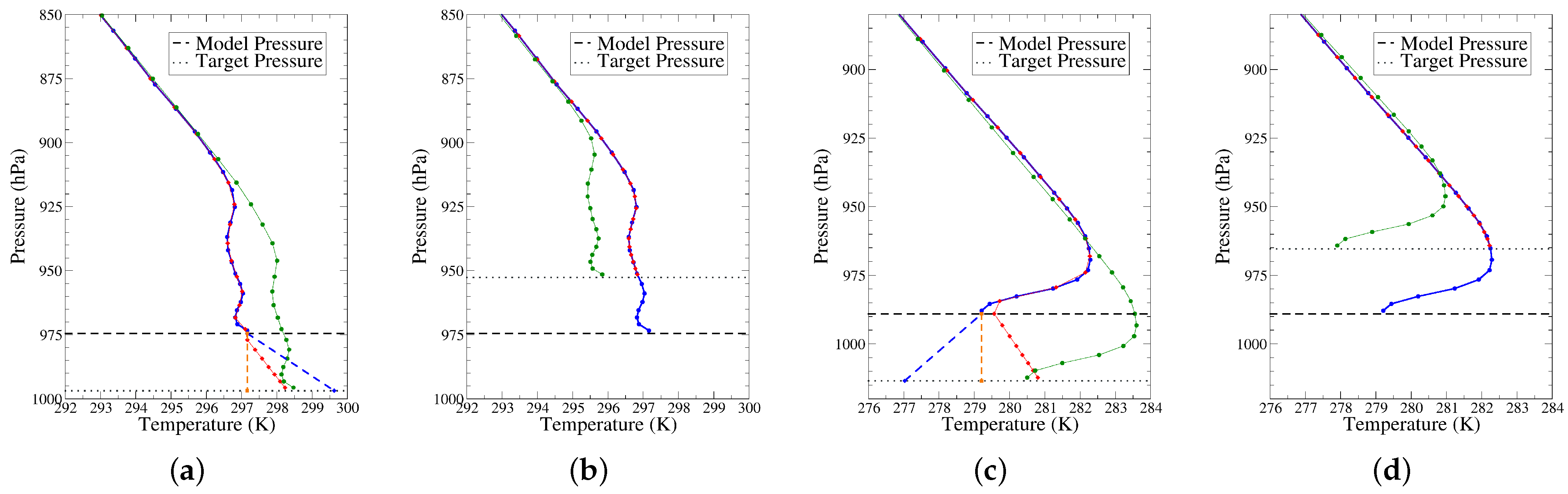
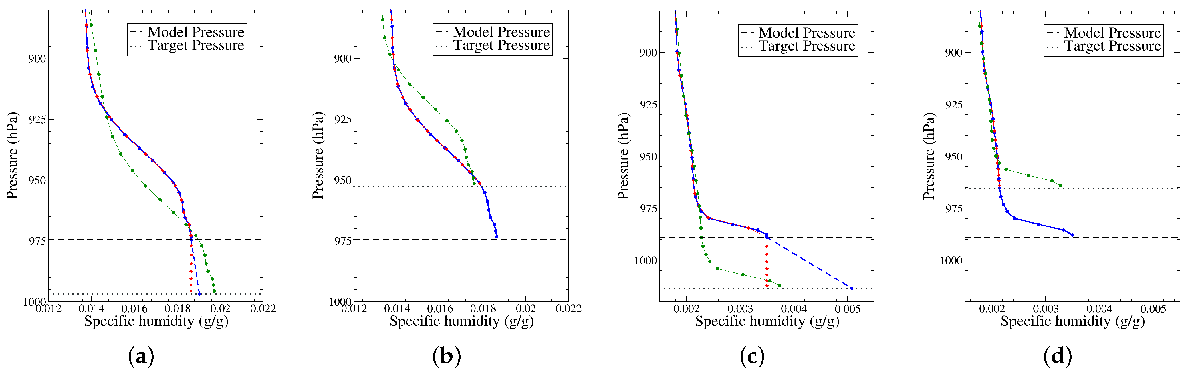
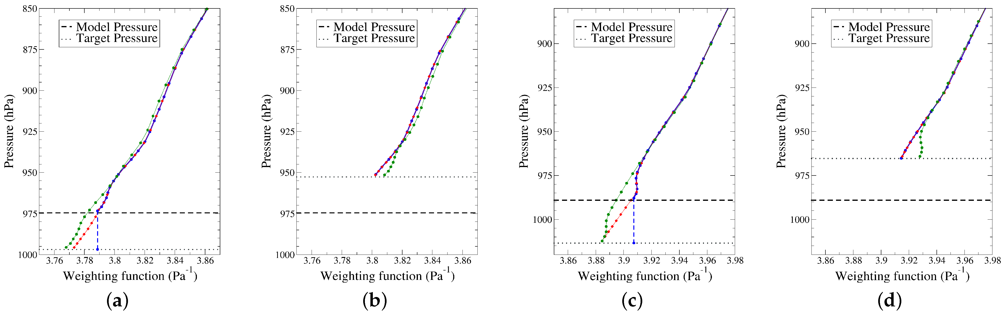
2.4. Vertical Interpolation and Extrapolation under the Model Topography

2.4.1. Different Methods

Vertical interpolations are performed to adapt the meteorological data to ${\Phi }_{DEM}$: the actual topography provided by a DEM (Digital Elevation Model). In order to determine $P{s}_{DEM}$, the pressure corresponding to ${\Phi }_{DEM}$ (the ground elevation at the target point), on the one hand, and the temperature and humidity values at the predefined pressure levels as a function of $P{s}_{DEM}$, on the other hand, interpolations are used between the vertical levels. These interpolations are chosen linear in pressure for temperature and specific humidity, linear in log pressure for geopotential and reciprocally linear in geopotential for log pressure. They are performed in terms of departures from the standard atmosphere (Appendix A) for increased accuracy [17]. Extrapolations are required to extend the profiles below the model topography when the target is below.

Four extrapolation methods are considered in this paper. Three of them differ in the gradient used to extrapolate the temperature and humidity profiles. For the first one, the gradient is chosen to be zero: it is assumed that the values of the layer just above the model floor are representative of the layer below the ground up to the target altitude. The last layer just at the level of the model ground is extended up to the actual ground. For the second one, the gradient is computed from the difference between the lowest layers of the atmospheric model. The extension is carried out taking into account the gradient between the second last and the last layer.

These first two extrapolations are physically relevant only if the difference between ${\Phi }_{NWP}$ and ${\Phi }_{DEM}$ is small. Unfortunately, this is not the case. Figure 2 shows the differences in topography for a full orbit between the ECMWF model at a resolution of about 10 km and the EarthEnv data at a resolution of 90 m. In a region such as the Alps, where the relief varies greatly, the differences can be over 1 km, while for flatter regions, the differences remain in the order of 20 m. It should be noted that over the sea, the differences are generated by Gibbs waves due to the spectral fit of the model topography, but they do not exceed one metre.

For the third extrapolation method, detailed in Appendix B, the temperature gradient below the ground is that of the standard atmosphere and the specific humidity gradient is zero. This third method is close to the way operational meteorological centres proceed [18] to post-process their data. When the difference in topography is large, it is better to use a standard value for the gradients instead of zero or an estimate computed very near the ground.

The fourth method, described in Appendix C, uses an unpublished approach developed at Météo-France for interpolations between different resolutions of the operational model ARPEGE (Action de Recherche Petite Echelle et Grande Echelle), hence its name APACHE (ARPEGE Pour ARPEGE CHamp Echangé) [19]. Its objective is to preserve a boundary layer close to the ground, both when the target topography is lower than the initial topography and in the opposite case. The idea is to retain certain quantities in the near-ground layers that are characteristic of the physical interactions between the atmosphere and the ground. The APACHE method preserves the potential temperature gradient related to the stability of the atmosphere and the relative humidity which is assumed to be more independent of temperature than the specific humidity and more characteristic of the balance between physical processes.

Table 1. Main characteristics of the different vertical interpolation methods.

Method	Zero Gradient	Last Gradient	Standard Gradient	APACHE
Extrapolation with	zero gradient	gradient determined from the latest levels of the weather model	standard gradient
Conservative properties				potential temperature gradient and relative humidity
Resampling	no	no	yes	yes

summarises the main features of the four vertical interpolation methods used.

2.4.2. Comparison of the Different Methods on Two Examples

To document the differences between the different vertical extrapolation, let us examine the temperature and humidity profiles produced by the different extrapolation methods in two cases, one above Africa and the other above the Alps, when the target elevation is set arbitrary 200 m below (Figure 3a,c) or above (Figure 3b,d) the model topography.

When the actual ground is below the model ground, the use of a non-standard gradient leads to unrealistic temperatures extrapolations near the actual ground. As expected, only the APACHE approach maintains an inversion near the actual ground whether it is above or below the model ground.

Similarly for humidity, Figure 4 shows the different methods of extrapolations. There is a risk of creating oversaturated humidities when using the last gradient (negative humidity can also occur in that case) and more generally when the specific humidity is maintained but the temperature is decreased. This is why APACHE maintains the relative humidity rather than the specific humidity. Finally, the APACHE approach again shows its advantage in preserving the structure of the boundary layer near the ground.

2.5. Intrinsic Uncertainties in Weather Forecasts

Furthermore, regardless of these interpolation issues, our knowledge of the meteorological fields is subject to errors that are generally estimated from the statistics of the differences between the model and the observations. A CNES study [20], based on ECMWF data from 2006, estimates for surface pressure, a bias of 0.2 hPa and a random error of 2 hPa; for temperature, a bias between $-0.2$ K and $0.2$ K (varying with vertical) and a random error of 2 K; and for specific humidity, a bias of 4% and a standard error of 15%. With these estimates, in the case of MERLIN, Bousquet et al. [1] attribute to the NWP data 7 ppb (8%) out of the 33 ppb estimated for the total random error and 0.7 ppb (6%) out of the 6.4 ppb estimated for the total systematic error. However, this statistical approach neglects error correlations both between vertical levels and between variables. For this reason, we have chosen another approach based on ensemble forecasting tools [21]. ECMWF generates every 12 H a set of fifty analyses compatible with the uncertainties of the forecast used as a first guess and those of the observations available [22]. These fifty perturbed forecasts were used in this study to provide an estimate of the uncertainty of the actual state of the atmosphere with respect to the unperturbed initial-state forecast used as reference. With our LIDSIM software, we have simulated the MERLIN signals from the atmospheric data of the reference forecast. Then, we have used each of the fifty perturbed forecasts in turn to obtain a estimate of the mole fraction of methane with respect to dry air averaged over the atmospheric column with the PROLID software, by computing $W{F}_G\left(p\right)$, the weighting functions for each gas, following Equation (3).

3. Results

3.1. Time Interpolation and Tide Waves

We have decided to use the weather data available every 3 h in the MARS database and to interpolate them linearly. However, it has been highlighted by work carried out by the CNES [20,23] that using model outputs at the hourly frequency leads to systematic differences between the pressure fields predicted at time H and interpolated between H − 2 and H + 1, whether using linear interpolation or a cubic spline. The differences interpreted as being related to the representation of atmospheric tides may induce regional biases up to 3 ppm on the mole fraction of methane with respect to dry air averaged over the atmospheric column (see Figure 5). Indeed, time interpolation creates systematic errors for insufficiently sampled periodic components such as atmospheric tides, as it is well documented in other contexts [24].

3.2. Impact on the Methane Retrieval of Vertical Interpolation Methods

We used several methods to adapt the atmospheric profiles corresponding to a particular ground altitude to another ground altitude. With LIDSIM, we compute the temperature and humidity profiles from the ECMWF data for a vertical pressure grid defined from the pressure value estimated at the DEM value, using one of the interpolation methods described above and detailed in Appendix B and Appendix C. In addition, we use these profiles to simulate the MERLIN data. Then, with PROLID, we invert the simulated signals using profiles constructed with another method. In all cases, except the “last gradient” case, a “zero gradient” method is used to extrapolate data from the DEM value to the SSE. There is no reason to use a more sophisticated method because the difference between the DEM value and the SSE is small except in the cloud cases, but then the boundary layer should not be moved as the SSE does not represent the ground.

The calculation of the IWF (Integrated Weighting Function, see Equation (3)) for a particular temperature and humidity profile, even if the surface pressure is fixed, depends on the distribution of the levels over the vertical. As explained in Appendix B and Appendix C, the “standard gradient” and APACHE methods change the discretisation of the profiles above the pressure determined at the DEM altitude (they resample atmospheric levels). However, the implementation of the “last gradient” and “zero gradient” methods is performed without level resampling. The deviation of the IWF due to the resampling could be measured. Expressed as a maximum error in the mole fraction of methane to dry air averaged over the atmospheric column, it corresponds to 0.08 ppb. This value is in agreement with an estimate we made (not shown) on five representative atmospheres from the TIGR database [25] and which shows that the difference between the exact calculation of the IWF and its approximation with a discretisation on 137 levels (vertical resolution of the ECMWF data used) is of the order of 0.04 ppb. This order of magnitude is also the contribution of the region above 40 km which is not taken into account in LIDSIM although its contribution will be present in the satellite data.

For the two points used for Figure 3 and Figure 4, the methane Weighting Function (see Equation (3)) is computed for the various interpolations both for a target above and below the model topography (see Figure 6).

By using a different extrapolation/interpolation method in LIDSIM and in PROLID, it is possible to estimate the order of magnitude of the error due to these extrapolations/interpolations. For the points considered above, whether the target is above or below the model topography, variations in the IWF (Integrated Weighting Function) induce uncertainties on the mole fraction of methane to dry air averaged over the atmospheric column of no more than 0.32 ppb.

Table 2. The standard deviation and the absolute maximum of the difference on the mole fraction of methane to dry air averaged over the atmospheric column in ppb according to the extrapolation methods used by LIDSIM and by PROLID. The mean is in all cases the same and its value of 0.08 ppb can be attributed to factors other than the meteorological data. The simulation is for a complete orbit. It is based on meteorological data from 6 May 2019 between 3:30 UT and 5:08 UT and on realistic reflectivity data (for more details, see Cassé et al. [6]) but assumes a constant value of 1780 ppb for methane content. Although there is no simulation of instrumental noise, due to the limited numerical accuracy when encoding the file representing the data transmitted to the ground segment, filtering of shots with a signal-to-noise ratio greater than 1 is necessary to eliminate the shots for which there is no signal.

	Extrapolation in LIDSIM with
Extrapolation in PROLID with	Zero Gradient	Last Gradient	Standard Gradient	APACHE
zero gradient		0.239/11.3	0.091/5.93	0.112/2.90
last gradient
standard gradient		0.266/13.1	0.063/0.30	0.114/2.85
APACHE		0.268/12.3	0.100/3.17	0.066/0.34

shows results for a complete orbit, the one whose topography on its ground track has already been shown in Figure 2a.

The results are optimal when we use the same method in LIDSIM and in PROLID. This simply means that the more our method matches what is happening in our environment, the better the results. Using the “last gradient” method in LIDSIM leads to thermodynamic profiles with extreme values that cannot be obtained with the other approaches.

The discrepancies are located in areas where the topography is highly variable. Otherwise, there is little difference in topography between the DEM and the meteorological model, which generates no significant difference in the methane estimates. Focusing on situations where the topography gap is large, the “standard gradient” method is preferred to the “zero gradient” method for PROLID because the latter gives strongly different values, as expected.

Figure 7a shows, as a function of the difference in topography between the meteorological model and the DEM, the differences between the mole fraction of methane to dry air averaged over the atmospheric column values retrieved by crossing between LIDSIM and PROLID the “standard gradient” method and the APACHE method. The error due to interpolation can be estimated, even if the real profiles are not known, from the dispersion of the results given by the different interpolation methods. This dispersion leads to differences of 1 ppb on the mole fraction of methane to dry air averaged over the atmospheric column when the topography correction reaches 200 m. However, examination of their distribution (Figure 7b) shows that the vertical interpolation error can be estimated at 0.0 ± 0.1 ppb.

To summarise, the impact on methane retrieval of the uncertainties in the way surface pressure as well as temperature and humidity profiles are adapted to another topography than the model topography is less than 3 ppb everywhere (even when the change in topography is more than 1 km). This value is obtained from Figure 7a before it is truncated at topographic deviations of ±200 m. The additional standard deviation is less than 0.1 ppb but with a systematic part at a particular location.

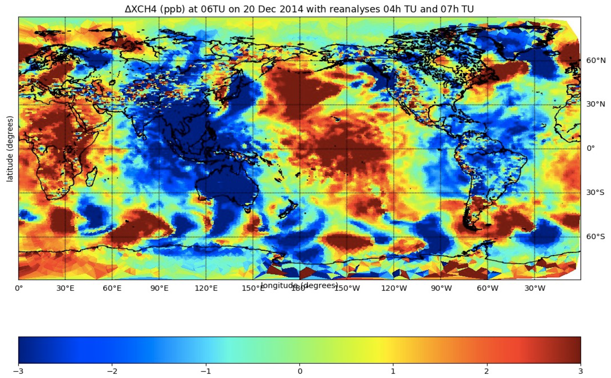
3.3. Sensitivity to the Analysis Errors

As explained above, we simulated the MERLIN data in LIDSIM using the ECMWF description of the atmosphere from the unperturbed initial state and inverted these data in PROLID using the other fifty descriptions of the atmosphere corresponding to forecasts from the perturbed states. We used data from 6 May 2019 between 03 UT and 06 UT. We present the results for the same orbit as above. In LIDSIM, we did not add instrumental noise to see only the impact of the NWP data. In LIDSIM and PROLID, we used the standard method to adjust the data to the DEM value.

Figure 8 shows the mean and the standard deviation of the fifty differences between $XC{H}_4^r$ (the mole fraction of methane to dry air averaged over the atmospheric column) obtained with Equation (1) for a set of meteorological parameters and its reference value [6]. This reference is defined as the pressure-averaged actual methane content provided by ECMWF with the weighting function ${WF}_{C{H}_4}\left(p\right)$ calculated for the set of meteorological parameters from the unperturbed initial state. The mean bias is of −0.03 ± 0.39 ppb and the mean standard deviation is of 0.58 ± 0.27 ppb.

Along the orbit, the dispersion of the differences in surface pressure ( respectively in total water vapour) with respect to the values of the forecast from the initial unperturbed state is shown in Figure 9 (respectively in Figure 10).

The fifty initial perturbations at 00 TU are symmetrical in pairs, but the integration of the model up to the observation time introduces many non-linearities that break this symmetry. This is why the average difference is not zero. Over the whole simulated orbit, for the surface pressure, the mean bias is 0.95 ± 12.65 Pa and the mean standard deviation is 17.96 ± 9.48 Pa, and for the total amount of water vapour expressed in Pa, the mean bias is −0.38 ± 7.22 Pa and the mean standard deviation is 6.82 ± 5.62 Pa.

We calculated the correlation coefficient (r) between the methane error standard deviation series ($X{\left(i\right)}_{i=1,N}$) and the pressure error standard deviation series ($Y{\left(i\right)}_{i=1,N}$). $r=\frac{E\left(\right(X-E\left(X\right)\left)\right(Y-E\left(y\right))}{{\sigma }_{X}s{\sigma }_Y}=\frac{E\left(XY\right)-E\left(X\right)E\left(Y\right)}{{\sigma }_{X}s{\sigma }_Y}$. We obtained a correlation factor of 0.86. Then, we compute the correlation coefficient between the methane error standard deviation series minus the pressure error series multiplied by the previous regression coefficient and the total water vapour error standard deviation series. This new correlation is also 0.86. These correlations can be interpreted in terms of explained variance. The variance from the meteorological uncertainties in $XC{H}_4$ is explained to 50% by the uncertainty in the surface pressure and to 25% by that in the water vapour. The rest is due to variations in temperature and vertical humidity distribution.

4. Discussion

4.1. Forecasting Errors

In order to compare our results regarding the impact of NWP data accuracy on the methane retrieval accuracy with those of Bousquet et al. [1], one must take into account the large difference in the estimates of systematic and random errors in the surface pressure used as input: 1 Pa and 18 Pa (see Figure 9) in this study instead of 20 Pa and 200 Pa in Bousquet et al. (i.e., almost 10 times less). Revisiting the 2006 data on the differences between observations and meteorological analyses, which were used to determine the Bousquet et al. values, we find that: globally at sea, compared to buoy measurements in the northern hemisphere, the pressure bias was 0.2 Pa and the standard deviation was 44 Pa, while on land, compared to aeronautical station data, the pressure bias was −11 Pa and standard deviation 60 Pa. Therefore, the values established in the CNES study [20] and used by Bousquet et al. [1] seem pessimistic. In 2011, Kiemle et al. [26] state that the random pressure error is less than 100 Pa in agreement with the Dee et al. [27] estimate around 70 Pa. The different values can be also explained by the regular improvement of forecast quality which continues up to now. The data available in the ECMWF website indicate an analysis bias of 3 Pa and a random error of less than 50 Pa for these last years. The estimate derived from the ensemble forecast is therefore representative of the state of the art, especially as our single orbit assessment necessarily underestimates the variability somewhat.

Given the advances in numerical weather prediction, the random error estimated by Bousquet et al. [1] at 7 ppb for the mole fraction of methane to dry air averaged over the atmospheric column can be reduced to 0.6 ppb and the bias from 0.7 ppb to 0.4 ppb, i.e., a gain of nearly 8% over the total random error and 3% over the total systematic error. However, we have to consider the differences between the actual observed profiles and those that can be estimated from the numerical forecasting data, which are not accounted for in this experiment. This is why we discuss the contribution of the various interpolations in the following.

4.2. Horizontal Interpolations

For our application, bilinear interpolations at a fixed vertical level of the NWP model are satisfactory. Although the quality of such a simple approach is often questioned, as there are many other ways to perform these interpolations, bilinear interpolations offer an excellent compromise between simplicity and accuracy. Alternatively, polynomial interpolations can be used to ensure multi-order derivability. However, they may be expensive to determine and subject to oscillations as their degree increases (Runge phenomenon). It is often preferable to use splines that are piecewise polynomials and to increase the number of polynomial pieces instead of increasing the degree of the polynomials used. Linear splines are obviously identical to the linear interpolation performed. Quadratic splines are rarely used in practice because with three degrees of freedom per interval, in dimension one, they require an additional constraint per interval which is not easy to fix objectively and the results are very dependent on this choice. Only cubic splines are used in certain circumstances. However, in their basic version, they require, in dimension two, sixteen points to determine the required first derivatives by finite difference, and they present problems with preserving extrema which can lead to negative values for humidity, for example. Nevertheless, it should be noted that where high accuracy is required, as in the case of using the semi-Lagrangian technique in a numerical model, there are several ways to save computational time and ensure extrema preservation [16]. However, there is no reason to use here these elaborate methods because of the inherent uncertainties in the quantities processed and because we have not identified any case in which a systematic error can occur.

4.3. Vertical Extrapolations

For the vertical extrapolations, systematic deviations may occur related to the method applied. Figure 7 shows that even for small differences in topography, different post-processing of the meteorological data can lead to deviations of 0.1 ppb in the vertically averaged methane concentration retrieval. Although it will be possible, on the basis of Figure 7a, to filter out the most important uncertainties by using a threshold on the topography differences between the meteorological model and the DEM; we assume a standard deviation error of 0.1 ppb due to these vertical interpolations.

4.4. Time Interpolations

The main concern with time interpolation is to avoid systematic errors due to periodic forcings with periods shorter than one day which are poorly represented by linear interpolation between two instants. We have identified the diurnal and semi-diurnal atmospheric tides and using a three-hourly sampling is not a sufficient representation of these waves. In the processing of altimeter data for the calculation of the pressure correction, the mean atmospheric tides are subtracted from the pressure field before time interpolation and its component calculated exactly at the target time is then added [28]. Unfortunately, this approach is more difficult to implement in our case as we not only have to interpolate the pressure field but also the temperature and humidity fields which are 3D fields. We plan to investigate how to deal with this problem in the future, as further research on this issue is needed, with the challenge of minimising local biases on retrieved methane.

5. Conclusions

We would have liked to recommend for the MERLIN ground segment to use the ECMWF operational analysis data available every three hours and to interpolate them linearly in time. However, we cannot do this until a method is validated to deal with atmospheric tides because of the regional bias they may induce. In addition, we need to plan specific work on this issue. There is no specific problem expected with the use of bilinear interpolations on the horizontal surfaces of the model. For the vertical extrapolation, only the “standard gradient” method or the APACHE method should be used in the MERLIN data processing due to the possible large differences between the topography of the meteorological model and the actual topography. The APACHE extrapolation method appears to be physically more consistent, but using simulated data, it is not possible to demonstrate a significant contribution to MERLIN data processing. Work will need to be performed during the flight commissioning phase, especially in areas with highly variable topography to analyse methane variations according to the interpolation method used. We plan to study this point with airborne data from the CHARM-F instrument [29] deployed during the MAGICS campaign [30].

With the exception of the atmospheric tides problem, meteorological uncertainties to the values used in the ground segment are expected to contribute at most 0.4 ppb to the bias in methane retrieval from MERLIN data and 0.7 ppb to its standard deviation, while uncertainties related to instrumental noise for 50 km averages of the mole fraction of methane to dry air averaged over the atmospheric column correspond to a bias of 1.2 ppb and a standard deviation of 16 ppb [6]. With appropriate atmospheric tides processing, the MERLIN instrument will be therefore at the breakthrough performance level of 2 ppb for systematic errors and 18 ppb for random errors.

References

1. Bousquet, P.; Pierangelo, C.; Bacour, C.; Marshall, J.; Peylin, P.; Ayar, P.V.; Ehret, G.; Bréon, F.M.; Chevallier, F.; Crevoisier, C.; et al. Error Budget of the MEthane Remote LIdar missioN and Its Impact on the Uncertainties of the Global Methane Budget. JGR Atmos. 2018, 123, 766–785. [Google Scholar] [CrossRef]
2. Myhre, G.; Shindell, D.; Bréon, F.-M.; Collins, W.; Fuglestvedt, J.; Huang, J.; Koch, D.; Lamarque, J.-F.; Lee, D.; Mendoza, B.; et al. Anthropogenic and Natural Radiative Forcing. In Climate Change 2013: The Physical Science Basis. Contribution of Working Group I to the Fifth Assessment Report of the Intergovernmental Panel on Climate Change; Stocker, T.F., Qin, D., Plattner, G.-K., Tignor, M., Allen, S.K., Boschung, J., Nauels, A., Xia, Y., Bex, V., Midgley, P.M., Eds.; Cambridge University Press: Cambridge, UK; New York, NY, USA, 2013; Available online: https://www.ipcc.ch/site/assets/uploads/2018/02/WG1AR5_Chapter08_FINAL.pdf (accessed on 18 February 2022).
3. Ehret, G.; Bousquet, P.; Pierangelo, C.; Alpers, M.; Millet, B.; Abshire, J.B.; Bovensmann, H.; Burrows, J.P.; Chevallier, F.; Ciais, P.; et al. MERLIN: A French-German Space Lidar Mission Dedicated to Atmospheric Methane. Remote Sens. 2017, 9, 1052. [Google Scholar] [CrossRef] [Green Version]
4. Nikolov, S.; Wührer, C.; Kühl, C.; Bode, M.; Hupfer, W.; Lucarelli, S. MERLIN: Design of an IPDA LIDAR instrument. CEAS Space J. 2019, 11, 437–457. [Google Scholar] [CrossRef]
5. Wirth, M. (DLR, Oberpfaffenhofen, Germany). MERLIN ATBD: Algorithm Theoretical Basis Document Part 1/Top Level Algorithms for Primary L1/2 Products. MLN-PLDP-ATBD-90001-PI Version 1 Rev 2, published by CNES and DLR, Toulouse. 2018; unpublished internal document. [Google Scholar]
6. Cassé, V.; Armante, R.; Bousquet, P.; Chomette, O.; Crevoisier, C.; Delahaye, T.; Edouart, D.; Gibert, F.; Millet, B.; Nahan, F.; et al. Development and Validation of an End-to-End Simulator and Gas Concentration Retrieval Processor Applied to the MERLIN Lidar Mission. Remote Sens. 2021, 13, 2679. [Google Scholar] [CrossRef]
7. Han, G.; Gong, W.; Lin, H.; Ma, X.; Xiang, Z. Study on Influences of Atmospheric Factors on Vertical CO2 Profile Retrieving from Ground-Based DIAL at 1.6 μm. IEEE Trans. Geosci. Remote Sens. 2015, 53, 3221–3234. [Google Scholar] [CrossRef]
8. Buchwitz, M.; Reuter, M.; Bovensmann, H.; Pillai, D.; Heymann, J.; Schneising, O.; Rozanov, V.; Krings, T.; Burrows, J.P.; Boesch, H.; et al. Carbon Monitoring Satellite (CarbonSat): Assessment of atmospheric CO2 and CH4 retrieval errors by error parameterization. Atmos. Meas. Tech. 2013, 6, 3477–3500. [Google Scholar] [CrossRef] [Green Version]
9. Ehret, G.; Kiemle, C.; Wirth, M.; Amediek, A.; Fix, A.; Houweling, S. Space-borne remote sensing of CO2, CH4, and N2O by integrated path differential absorption Lidar: A sensitivity analysis. Appl. Phys. B Lasers Opt. 2008, 90, 593–608. [Google Scholar] [CrossRef] [Green Version]
10. Jacquinet-Husson, N.; Armante, R.; Scott, N.A.; Chedin, A.; Crépeau, L.; Boutammine, C.; Bouhdaoui, A.; Crevoisier, C.; Capelle, V.; Boonne, C.; et al. The 2015 edition of the GEISA spectroscopic database. J. Mol. Spectrosc. 2016, 327, 31–72. [Google Scholar] [CrossRef] [Green Version]
11. Delahaye, T.; Maxwell, S.E.; Reed, Z.D.; Lin, H.; Hodges, J.T.; Sung, K.; Devi, V.; Warneke, T.; Tran, H. Precise methane absorption measurements in the 1.64 μm spectral region for the MERLIN mission. JGR Atmos. 2016, 121, 7360–7370. [Google Scholar] [CrossRef] [PubMed]
12. Delahaye, T.; Ghysels, M.; Hodges, J.T.; Sung, K.; Armante, R.; Tran, H. Measurement and modeling of air-broadened methane absorption in the MERLIN spectral region at low temperatures. JGR Atmos. 2019, 124, 3556–3564. [Google Scholar] [CrossRef]
13. ECMWF, MARS—The ECMWF Meteorological Archive. Available online: https://www.ecmwf.int/node/18124 (accessed on 18 February 2022).
14. ECMWF. IFS Documentation Cy47r1, Part II: Data Assimilation; ECMWF: Reading, UK, 2020. [Google Scholar] [CrossRef]
15. Robinson, N.; Regetz, J.; Guralnick, R.P. EarthEnv-DEM90: A nearly-global, void-free, multi-scale smoothed, 90 m digital elevation model from fused ASTER and SRTM data. ISPRS J. Photogramm. Remote Sens. 2014, 87, 57–67. [Google Scholar] [CrossRef]
16. ECMWF. IFS Documentation Cy47r1, Part III: Dynamics and Numerical Procedures; ECMWF: Reading, UK, 2020. [Google Scholar] [CrossRef]
17. Simmons, A.J.; Chen, J. The calculation of geopotential and the pressure gradient in the ECMWF atmospheric model: Influence on the simulation of the polar atmosphere and on temperature analyses. Q. J. R. Meteorol. Soc. 1991, 117, 29–58. [Google Scholar] [CrossRef]
18. ECMWF. IFS Documentation Cy47r1, Part I: Observations; ECMWF: Reading, UK, 2020. [Google Scholar] [CrossRef]
19. Bubnová, R. Pouziti Souradnice “Hydrostaticky Tlak” pro Integraci Elastického Modelu Dynamiky Atmosféry v Numerickém Predpovednim Systému ARPEGE/ALADIN. Ph.D. Thesis, Paul Sabatier University, Toulouse, France, Charles University, Prague, Czech Republic, 25 April 1995. [Google Scholar]
20. Chinaud, J.; Pierangelo, C.; Tyrou, V.; Millet, B. (CNES, Toulouse, France). MERLIN Level 2 error budget. MLN-SYS-TN-0399-CNS, Issue 5. 2021; unpublished internal document. [Google Scholar]
21. ECMWF. IFS Documentation Cy47r1, Part V: Ensemble Prediction System; ECMWF: Reading, UK, 2020. [Google Scholar] [CrossRef]
22. Isaksen, L.; Bonavita, M.; Buizza, R.; Fisher, M.; Haseler, J.; Leutbecher, M.; Raynaud, L. Ensemble of Data Assimilations at ECMWF; Technical Report 636; ECMWF: Reading, UK, 2010. [Google Scholar] [CrossRef]
23. Martins, E.; Chinaud, J. Impact of the interpolation of the meteorological profiles on XCH4 retrievals. «Groupe Mission MERLIN» Meeting, LMD Palaiseau (France). 2020; unpublished internal document. [Google Scholar]
24. Li, Z.; Chen, W.; Jiang, W.; Deng, L.; Yang, R. The Magnitude of Diurnal/Semidiurnal Atmospheric Tides (S1/S2) and Their Impacts on the Continuous GPS Coordinate Time Series. Remote Sens. 2018, 10, 1125. [Google Scholar] [CrossRef] [Green Version]
25. Chevallier, F.; Chédin, A.; Chéruy, F.; Morcrette, J.-J. TIGR-like atmospheric-profile databases for accurate radiative-flux computation. Q. J. R. Meteorol. Soc. 2000, 126, 777–785. [Google Scholar] [CrossRef]
26. Kiemle, C.; Quatrevalet, M.; Ehret, G.; Amediek, A.; Fix, A.; Wirth, M. Sensitivity studies for a space-based methane lidar mission. Atmos. Meas. Tech. 2011, 4, 2195–2211. [Google Scholar] [CrossRef] [Green Version]
27. Dee, D.P.; Uppala, S.M.; Simmons, A.J.; Berrisford, P.; Poli, P.; Kobayashi, S.; Andrae, U.; Balmaseda, M.A.; Balsamo, G.; Bauer, P.; et al. The ERA-Interim reanalysis: Configuration and performance of the data assimilation system. Q. J. R. Meteorol. Soc. 2011, 137, 553–597. [Google Scholar] [CrossRef]
28. Ray, R.D.; Ponte, R.M. Barometric tides from ECMWF operational analyses. Ann. Geophys. 2003, 21, 1897–1910. [Google Scholar] [CrossRef] [Green Version]
29. Amediek, A.; Ehret, G.; Fix, A.; Wirth, M.; Budenbender, C.; Quatrevalet, M.; Kiemle, C.; Gerbig, C. CHARM-F a new airborne integrated-path differential-absorption lidar for carbon dioxide and methane observations: Measurement performance and quantification of strong point source emissions. Appl. Opt. 2017, 56, 5182–5197. [Google Scholar] [CrossRef] [PubMed]
30. Crevoisier, C.; Bes, C.; Joly, L.; Té, Y.; Ramonet, M.; Herbin, H.; Catoire, V.; Fix, A.; Cézard, N.; Bourdon, A.; et al. Overview of the MAGIC Initiative for GHG and Future Plans. In Proceedings of the International Workshop on Greenhouse Gas Measurements from Space, IWGGMS-17, Online Conference, 15 June 2021; Available online: https://cce-datasharing.gsfc.nasa.gov/files/conference_presentations/Talk_Crevoisier_148_25.pdf (accessed on 18 February 2022).
31. COESA (Committee on Extension to the Standard Atmosphere). U.S. Standard Atmosphere, 1976; U.S. Government Printing Office: Washington, DC, USA, 1976. Available online: https://www.ngdc.noaa.gov/stp/space-weather/online-publications/miscellaneous/us-standard-atmosphere-1976/us-standard-atmosphere_st76-1562_noaa.pdf (accessed on 18 February 2022).
32. Simmons, A.J.; Burridge, D.M. An energy and angular momentum conserving vertical finite difference scheme and hybrid vertical coordinates. Mon. Weather Rev. 1981, 109, 758–766. [Google Scholar] [CrossRef] [Green Version]
33. ECMWF. IFS Documentation Cy47r1, Part IV: Physical Processes; ECMWF: Reading, UK, 2020. [Google Scholar] [CrossRef]
34. Buck, A.L. New Equations for Computing Vapor Pressure and Enhancement Factor. J. Appl. Meteorol. Climatol. 1981, 20, 1527–1532. [Google Scholar] [CrossRef] [Green Version]
Figure 1. (a) Schematic of time and horizontal interpolations. An observation is made at time t i between times t and t’ corresponding to the times when meteorological data are available. V 1 , V 2 , V 3 , V 4 are the value of a parameter at four points around the target point at time t and V 1 , V 2 , V 3 , V 4 are the value at the same points at time t’. V i is the interpolated value at the target point at time t i . (b) For the Corsica region, on a representation of the topography from the EarthEnv DEM [15], the points where meteorological data are available in the ECMWF database are in red and the target points that are part of the MERLIN ground track are in black.
Atmosphere 13 00431 g001
Figure 2. Comparison between the meteorological model topography (red) and the numerical elevation model used [15] (blue). The difference is in green. (a) For a complete orbit starting north of Canada, descending over the Pacific to Antarctica, ascending over Africa and the Alps, before ending over Greenland. The shot index corresponds to the position in the simulated orbit. (b) A zoom on the Alps region where the difference sometimes exceeds 1 km. (c) A zoom on a flat area, the differences are about 20 m. (d) Over the sea, the differences are not zero because of the Gibbs phenomenon affecting the model topography, but they are less than 1 m.
Atmosphere 13 00431 g002
Figure 3. Temperature profiles provided by different extrapolations with zero gradient in orange, last gradient in blue, standard gradient in red and APACHE method in green. The original profile defined only above the model topography corresponds to the blue points above the model ground pressure. Two examples: the first one over Africa, the second over the Alps. (a,c) with a target below the model topography, (b,d) with a target above the model topography.
Atmosphere 13 00431 g003
Figure 4. Humidity profiles provided by different extrapolations with last gradient in blue, standard (zero) gradient in red and APACHE method in green. The original profile defined only above the model topography corresponds to the blue points above the model ground pressure. Two examples: the first one over Africa, the second over the Alps. (a,c) with a target below the model topography, (b,d) with a target above the model topography.
Atmosphere 13 00431 g004
Figure 5. Figure, made by Edouard Martins and Jordi Chinaud and reproduced with their kind permission, showing the difference at 06H UT for 20 December 2014 between the amount of methane obtained with the meteorological fields reanalysed at that time and that obtained with an interpolation between the meteorological fields reanalysed at 04H UT and 07H UT.
Atmosphere 13 00431 g005
Figure 6. Methane weighting functions obtained according to different extrapolations: with zero gradient in blue, standard gradient in red and APACHE method in green. Two examples: the first one over Africa, the second over the Alps. (a,c) with a target below the model topography. (b,d) with a target above the model topography.
Atmosphere 13 00431 g006
Figure 7. Distribution of the differences between the mole fraction of methane to dry air averaged over the atmospheric column retrieved using the “standard gradient” in LIDSIM and APACHE in PROLID and the same quantity retrieved using APACHE in LIDSIM and the “standard gradient” in PROLID. (a) Each point corresponds to such a difference distributed according to the difference in topography between the meteorological model and the DEM limited for the figure to ±200 m. (b) The histogram of these differences (with a sampling of 0.025 ppb): in green if the topography difference is between −50 m and 50 m, in red if it is greater than 50 m and in blue if it is less than −50 m. We have eliminated the points with a difference in topography between −10 m and 10 m for reasons of readability, which represents 72,333 points out of 95,360 that are with differences in methane retrieval of less than 0.1 ppb.
Atmosphere 13 00431 g007
Figure 8. Results for mole fraction of methane to dry air averaged over the atmospheric column for an orbit simulated without instrumental noise. Mean curve in black and area between ± one standard deviation in blue. The shot index corresponds to the position in the simulated orbit which topography as provided in Figure 2a.
Atmosphere 13 00431 g008
Figure 9. Discrepancies on the surface pressure. Mean curve in black and area between ± one standard deviation in blue.
Atmosphere 13 00431 g009
Figure 10. Discrepancies on the total amount of water vapour. Mean curve in black and area between ± one standard deviation in blue.
Atmosphere 13 00431 g010