Prediction of Carbon Emissions in China’s Power Industry Based on the Mixed-Data Sampling (MIDAS) Regression Model

Abstract

China is currently the country with the largest carbon emissions in the world, to which, the power industry contributes the greatest share. To reduce carbon emissions, reliable and timely forecasting measures are important and necessary. By using different frequency variables, in this study, we used the mixed-data sampling (MIDAS) regression model to forecast the annual carbon emissions of China’s power industry compared with a benchmark model. It was found that the MIDAS model had a higher prediction accuracy than models such as the autoregressive distributed lag (ARDL) model. Moreover, our results showed that the MIDAS model could conduct timely nowcasting, which is useful when the data have some releasing lag. Through this prediction method, the results also demonstrated that the carbon emissions of the power industry have a significant relationship with GDP and thermal power generation, and that the value of carbon emissions would keep increasing in the years of 2021 and 2022.

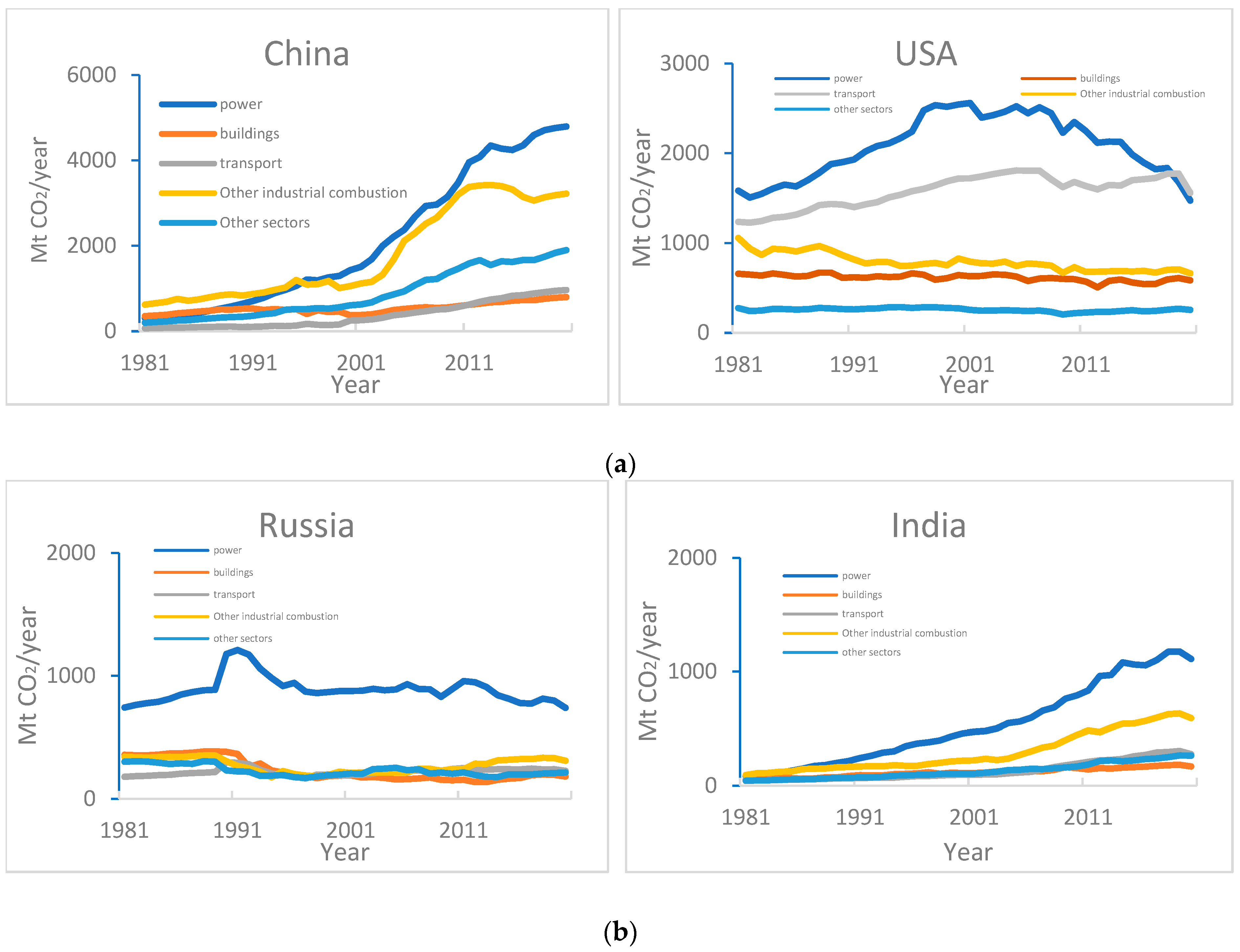
1. Introduction

Carbon emissions are one of the main by-products of industrial production and human life, of which, energy consumption is the main source. The increase in the Earth’s average temperature caused by carbon emissions has had a serious impact on ecological balance and climate stability. Therefore, energy conservation and emission reduction are consistent and urgent tasks worldwide. China is currently the country with the largest carbon emissions in the world. As the largest developing country, China’s carbon emissions show unique characteristics. First, China is the world’s largest carbon emitter in terms of total emission amounts. As a result, there has been much more pressure for energy conservation and emission reduction than in other countries, especially since China is still a developing country in terms of industrialization and urbanization. Secondly, from the perspective of structure, although the power industry also accounts for the highest proportion of carbon emissions in China compared with other major carbon emissions, the difference is that the carbon emissions of China’s power industry are still growing, whereas those of other countries are starting to decrease. It can be seen in Figure 1a,b, which shows the largest four countries in terms of carbon emissions across the world [1], that the power industry carbon emissions of the other three countries have peaked, but those of China have not.

This is mainly because China’s electricity is mainly generated by coal-fired thermal power plants, which omit a large amount of carbon dioxide and other greenhouse gases (GHG). Although thermal power plants have the advantages of a stable power supply, relatively lower impact from weather fluctuations, and less potential damage to the power grid, their carbon emissions have led to long-term high carbon emissions by the power industry. According to China’s National Bureau of Statistics (Beijing, China), China’s thermal power plants make up 74% of all power plants [2].

In September 2020, China proposed specific targets for carbon emission reductions, namely “peaking carbon dioxide emissions by 2030 and achieving carbon neutrality by 2060” [3]. As mentioned above, based on the characteristics of China’s carbon emissions, to achieve this goal, controlling the carbon emissions of the power industry is key. The power industry is the foundation of economic growth, so carbon emissions are closely related to GDP. On the basis of this hypothesis, our first attempt was to use GDP as an independent variable to predict the carbon emissions of the power industry. Moreover, the carbon emissions of the power industry are directly related to the amount of electricity generated by thermal power plants. Since these amounts can be controlled by a plan, if the relationship between carbon emissions and the electricity produced by the thermal power plant can be estimated, this will have more practical significance for the daily management of carbon emissions. Therefore, we first used GDP and thermal power generation as separate independent variables to predict the carbon emissions of the power industry, and then simultaneously used GPD and thermal power generation as multiple independent variables to predict the power industry’s carbon emissions.

The carbon emission data are released yearly, whereas the data on GDP and thermal power generation are published quarterly and monthly, respectively. To predict carbon emissions by using the data on GDP or thermal power generation, the first obstacle we faced was the difference in data frequency. Generally, if the data of the dependent variable and the independent variable are of different frequencies, mathematical processing is required to downgrade them to the same frequency, or else the low-frequency data are raised to high-frequency data by means of interpolation, data fitting, etc. The approach of adding up or averaging the low-frequency data will lose more useful original information and cause distortion in the predictions, which is one of the disadvantages of this approach. Moreover, for data with the same frequency, because there are usually time lags in releasing the data, it is difficult to make timely dynamic predictions or to update the predictions according to the latest data releases and establish an automatic prediction index. To solve these difficulties, Ghysels et al. [4] proposed the mixed-frequency model, which combines low-frequency data with high-frequency data by imposing a weighted function, and showed an improvement in the prediction of mixed-frequency data. Giannone et al. [5] found that, when current quarterly data were used to generate nowcasts of quarterly GDP data, the latest updated data and timely information helped to improve the forecasting accuracy. Today, when big data and machine learning are widely used, and the immediacy and accuracy of forecasts are increasingly required, the application of mixed-frequency models for carbon emission forecasting can be a useful model.

To carry out a comparative study, this research also used the ADRL model to predict the carbon emissions of the power industry to determine whether MIDAS had a better performance than the traditional model. The remainder of this article is arranged as follows: Section 2 reviews the methods of forecasting carbon emissions and expounds on the relevant literature and research on carbon emissions in China; Section 3 introduces the main principles and main applications of the MIDAS model and establishes the index of prediction accuracy; Section 4 describes the data sources and the preliminary processing of the data; and Section 5 compares and analyzes the performance of different models in forecasting. Finally, the conclusions and discussion end the article in Section 6 and Section 7, respectively.

2. Literature Review

Carbon emissions are closely related to industrial development and people’s lives. To reduce carbon emissions, we must first investigate the source of carbon emissions, then analyze the relationship between emissions and major economic variables, and then predict carbon emissions on the basis of this relationship. Many attempts to measure and predict carbon emissions have been made by many studies in the literature. Fang et al. [6] proposed an improved Gaussian process regression model to predict the total carbon dioxide emissions of several countries and found that some countries will still have increased emissions but others will be well controlled in the short term. Wu et al. [7] studied the impact of economic growth on carbon emissions in the BRICS countries (Brazil, Russia, India, China, and South Africa) by using a multi-variable grey model, and found that the impact of economic growth in Brazil and Russia on carbon emissions was getting smaller, whereas carbon emissions from India, China, and South Africa would increase. Chang et al. [8] proposed an algorithm based on combined quantum harmony search (QHS) to predict carbon emissions from fossil fuels. Köne et al. [9] used trend analysis to forecast the energy-related carbon emissions of the world’s top 25 emitting countries. Zhao et al. [10] used a MIDAS model and back propagation (BP) to study the impact of quarterly economic growth on annual carbon emissions, and the empirical results showed that economic growth has both negative and positive effects on carbon dioxide emissions across 15 quarters. Hosseini et al. [11] used multiple linear regression (MLR) and multiple polynomial regression (MPR) analyses to predict Iran’s carbon dioxide emissions in 2030 under two scenarios.

China is currently the country with the largest carbon emissions in the world, and there are many studies focusing on China’s carbon emissions. Fang et al. [12] used the stochastic impacts by regression on population, affluence, and technology (STIRPAT) model to predict whether China’s energy-related industries would peak in 2030, and the results showed that 26 provinces in China are likely to peak. Li et al. [13] combined the extreme learning machine and support vector machine algorithm (SVM-ELM) model and the grey prediction model (GM) to predict the carbon emissions of energy consumption in Beijing and its surrounding areas, which showed that the proportion of energy consumption has a serious impact on carbon emissions.

Some studies have conducted further research on carbon emissions, concentrating on industry carbon emissions. Lin et al. [14] used the logarithmic mean Divisia index (LMDI) decomposition method to analyze the carbon emissions of the chemical industry and believed that the factors of energy intensity and energy structure are beneficial for reducing the carbon emissions of the chemical industry. Fatima et al. [15] conducted a decomposition analysis of the change in China’s industrial carbon emissions and found that energy intensity and carbon emission effects were the most important factors for reducing carbon emissions. Yang et al. [16] used the ARIMA model to predict the carbon emissions of the aviation industry in Shanghai, China, and the results showed that the carbon emissions of the aviation industry will increase by 6.41% in June 2021. Zhang et al. [17] decomposed the main factors of carbon dioxide emissions from China’s logistics industry by establishing an extended LMDI model.

As mentioned above, most of the research has focused on exploring the relationship between economic growth and carbon emissions, but fewer studies have deeply explored the source of carbon emissions, especially from the perspective of industry. Moreover, despite it being the biggest carbon emission industry in China, little research has focused on predicting the carbon emissions of the power industry. Moreover, much research has used data with the same frequency, which is insufficient for including the necessary information and demonstrating timeliness. The main innovation of this present study is that it used data with different frequencies and the MIDAS model to predict the carbon emissions of China’s power industry for the first time, which enhanced the accuracy and timeliness of the predictions. Since the thermal power generation can be controlled and arranged by the authorities, this method could provide a practical path for managing carbon emissions in this industry.

3. Methodology

3.1. ARDL Model

In this study, we chose the ARDL model as a comparison or benchmark model for the MIDAS model, mainly because the MIDAS model was developed from the ARDL model. The general expression of an ADRL model is:

$$Y_t={\beta }_0+{\displaystyle \sum }_{j=1}^q{\beta }_j{Y}_{t-j}+{\displaystyle \sum }_{i=0}^p{a}_i{X}_{t-i}+u_t$$

(1)

In the above formula, $Y_t$ is the low-frequency dependent variable in period $t$, $X_t$ is the high-frequency independent variable, $Y_{t-j}$ is the dependent variable lag in period $j$, $X_{t-i}$ is the independent variable lag in period $i$, and $p$ and $q$ are the largest lag order of the independent and dependent variables, respectively, which is also written as an ARDL (q, p) model. The ARDL model is mostly used to predict the relationship between different time series. Some studies have used this model for the long-term relationships among monetary supply, income, nominal interest rates, foreign interest rates, and foreign exchange rates [18], and another study used this model to explore the long-term relationships between energy and economic growth in some countries [19]. Recently, many studies have used the ARDL model to study the relationships among economic growth, policy, and carbon emissions [20,21]. Since there are many high-frequency lag polynomials in the model that need to be estimated, some constraints, such as weight average, are often applied to estimation models, which led to the concept of the MIDAS model.

3.2. The MIDAS Model

As mentioned above, the MIDAS model was derived from ARDL model and is widely used when dependent variables and independent variables with different frequencies are used in the same model. Unlike other models, the MIDAS model can make full use of the information of high-frequency variables, restrict the coefficient to be evaluated, and improve the prediction accuracy of low-frequency variables. It was originally designed to predict stock market volatility. Accordingly, the MIDAS model was initially only a basic model with one independent variable, and then gradually developed into a multiple independent variate model.

3.2.1. The Basic MIDAS Model

The basic equation of the MIDAS model is:

$$Y_t={\beta }_0+{\beta }_{1}B\left(L^{1/m};\theta \right)X_t^{\left(m\right)}+{\epsilon }_t$$

(2)

where $Y_t$ is the low-frequency dependent variable, $X_{t-1}^{\left(m\right)}$ is the high-frequency independent variable, and $m$ is the frequency ratio between the high-frequency data and the low-frequency data. If $Y_t$ represents annual data and $X_t$ represents monthly data, then $m$ equals 4; if $Y_t$ represents quarterly data and $X_t$ represents monthly data, then $m$ equals 3, and so on. $B\left(L^{1/m}\right)$ is a weighted lag polynomial, which is the essence of this MIDAS model, and its expression is $B\left(L^{1/m};\theta \right)={{\displaystyle \sum }}_{k=0}^{K}B\left(k;\theta \right)L^{\raisebox{1ex}{$k$}\!\left/ \!\raisebox{-1ex}{$m$}\right.}$. $L^{\raisebox{1ex}{$1$}\!\left/ \!\raisebox{-1ex}{$m$}\right.}$ is a lag operator and satisfies $L^{\raisebox{1ex}{$1$}\!\left/ \!\raisebox{-1ex}{$m$}\right.}{x}_t^{\left(m\right)}=x_{t-\raisebox{1ex}{$1$}\!\left/ \!\raisebox{-1ex}{$m$}\right.}^{\left(m\right)}$. ${\beta }_0$ and ${\beta }_1$ are the parameters or coefficients to be estimated, and ${\epsilon }_t$ represents the i.i.d. error. The basic MIDAS model is described as the MIDAS (m, K) model.

MIDAS models are usually divided into constrained models and unconstrained models. Constrained models are those that apply a weighted lag polynomial because the selection of constraints is often subjective, which may lead to deviations in the estimated or predicted results. The unconstrained MIDAS model proposed by Foroni et al. [22], also known as the U-MIDAS model, does not need to impose constraints by using a lag polynomial and can directly use the least squares method for regression. The unconstrained MIDAS model is as follows:

$$Y_t={\beta }_0+{\displaystyle \sum }_{k=0}^K{\beta }_k{x}_{tm-k}+{\epsilon }_t$$

(3)

Constrained MIDAS models use very parsimonious distribution lags to describe the response of dependent variables to high-frequency independent variables, reducing the number of parameters from being too large and thus decreasing the difficulty of estimation. Expressing the coefficients of the lagged independent variables as a distributed lag function helps us to characterize the dependent variables. The weight function is used to constrain the variable coefficients. Ghysels [23] suggested the Almon polynomial, the exponential Almon polynomial, the beta polynomial, and other weighted polynomial functions. The expression of the Almon polynomial is expressed as:

$$\omega \left(k;\theta \right)={\theta }_0+{\theta }_{1}k+{\theta }_2{k}^2+\cdots {\theta }_p{k}^p/{{\displaystyle \sum }}_{k=1}^K\left({\theta }_0+{\theta }_{1}k+{\theta }_2{k}^2+\cdots {\theta }_p{k}^p\right)$$

(4)

The exponential Almon polynomial is expressed as follows:

$$\omega \left(k;\theta \right)=\exp \left({\theta }_0+{\theta }_{1}k+{\theta }_2{k}^2+\cdots {\theta }_p{k}^p\right)/{{\displaystyle \sum }}_{k=1}^K\exp ({\theta }_0+{\theta }_{1}k+{\theta }_2{k}^2+\cdots {\theta }_p{k}^p)$$

(5)

The beta polynomial is expressed as follows:

$$\omega \left(k;{\theta }_1,{\theta }_2\right)=f\left(k/K,{\theta }_1;{\theta }_2\right)/{\displaystyle \sum }_{k=1}^{K}f\left(k/K,{\theta }_1;{\theta }_2\right)$$

(6)

In these three equations, $K$ is the lag order of the independent variables and $\theta$ is the parameter of the polynomials.

Since the MIDAS model was proposed, it has made rapid progress. Götz et al. [24] combined the smooth transition model and the frequency mixing model to propose a model called the smooth transition mixing model (STMIDAS), which showed improvements in predictive ability for non-stationary series. Guérin et al. [25] proposed the Markov mixed data sampling regression model (MSMIDAS), which used state changes in the MIDAS parameters to predict economic activity in the United States. Foroni et al. [22] introduced MIDAS regression with unrestricted linear lag polynomials (U-MIDAS), which is particularly useful when the difference in the sampling frequency of the explanatory variable and the explained variable is small. Breitung et al. [26] introduced a non-parametric model into a MIDAS model to predict inflation problems.

In the initial and early stages, MIDAS was mainly used to predict characteristic financial market indicators by applying financial high-frequency data. Ghysels et al. [27] developed a MIDAS regression model for predicting stock returns. Forsberg et al. [28] found that the MIDAS model had the ideal overall forecasting properties for measure volatility based on stock returns. Alper et al. [29] used MIDAS to predict the weekly volatility of stock markets in 10 emerging markets, and the results showed that the prediction accuracy was higher than that of the generalized autoregressive conditional heteroskedasticity (GARCH) model. Körs [30] forecasted the volatility of stocks in 8 countries beyond 1 month, showing that the MIDAS model can be a sophisticated tool for predicting future volatility. With the development of the model, the MIDAS model was gradually applied in the prediction of macroeconomic indicators. Kuzin et al. [31] used MIDAS and vector autoregression (VAR) models to forecast GDP in the Euro area and found that MIDAS had more advantages for short-term forecasting. Pan et al. [32] used a time-varying parameter MIDAS model (TVP-MIDAS) to predict the real GDP growth of the United States by using crude oil prices and proved that it outperformed the ordinary least squares (OLS) regression model or the constant coefficient model. Li et al. [33] used Internet search data as high-frequency data, implementing the MIDAS model to predict China’s consumer price index (CPI), and proved that search data are strongly correlated with CPI. Gunay et al. [34] used different variables, such as quarterly GDP, monthly exports, and daily Brent crude oil prices, to predict the performance of the Chinese economy during COVID-19. MIDAS has also been used for carbon emissions. Chevallier [35] used the dynamic conditional correlation-mixed data sampling (DCC-MIDAS) model to demonstrate the negative impact of COVID-19 on US financial markets and carbon emissions.

3.2.2. Multiple Independent Variables MIDAS Model

It is often necessary to combine multiple independent variables to predict a macroeconomic indicator. If there are two or more high-frequency independent variables in MIDAS, we obtain the M(n)-MIDAS (m, K) model, which can be used to identify different coefficients between low-frequency variables and high-frequency variables. The M(n)-MIDAS (m, K) model with $n$ explanatory variables can be expressed as:

$$Y_t={\beta }_0+{\displaystyle \sum }_{i=1}^n{\beta }_i{B}_i\left(L^{\raisebox{1ex}{$1$}\!\left/ \!\raisebox{-1ex}{$m$}\right.};{\theta }_i\right)X_{i,t}^{\left(m\right)}+{\epsilon }_t$$

(7)

In the equation above, the number of independent low-frequency variables increases to $n$, compared with Equation (2).

3.2.3. The h-Step Ahead MIDAS Model

Generally, the release of statistical data has a lag. For example, the release time of quarterly GDP is generally in the first month after the end of the quarter, and the release time of the other annual data will be longer. In fact, the annual carbon emission data used in this article have a lag period of more than half a year. Compared with the same-frequency prediction model, the MIDAS model has the advantages of real-time prediction and gradual revision. Supposedly, when quarterly GDP is used to forecast annual carbon emissions, the first quarter’s GDP can be used to forecast carbon emissions for the current year, and when the second quarter’s GDP is announced, the previous two quarters’ data can be used immediately to revise the result. In this way, the latest information can be absorbed more frequently, and the forecasting can be updated and revised in real time. The formula for the h-step forward MIDAS model is:

$$Y_t={\beta }_0+{\displaystyle \sum }_{i=1}^n{\beta }_i{B}_i\left(L^{\raisebox{1ex}{$1$}\!\left/ \!\raisebox{-1ex}{$m$}\right.};{\theta }_i\right)X_{i,t-h/m}^{\left(m\right)}+{\epsilon }_t$$

(8)

where h is the advanced steps of the high-frequency data, indicating that the low-frequency variable is predicted at h steps forward. When h = 0, it means that both the high-frequency data and low-frequency data have been obtained, which is a real-time nowcast. In this study, h = 0 means that the forecast of the current year’s carbon emissions is based on the data of GDP and thermal power generation of four quarters of the same year. When h = 1, it means the data of the first three quarters were used, whereas h = 2 means that the data of the first two quarters were used, etc. When h = 4, the data of the current year were used to predict the carbon emissions of the next year, which is a long-term forecast.

3.3. Accuracy Index

In this study, we used the root mean square error (RMSE) as the measure to identify the forecast error and relative accuracy. The formula for calculating RMSE is:

$$RMSE=\sqrt{\frac{1}{m}{\displaystyle \sum }_{i=1}^m{\left(\widehat{y_i}-y_i\right)}^2}$$

(9)

The mean absolute proportional error (MASE) and the mean absolute percentage error (MAPE) can be used as auxiliary evaluation criteria.

$$MAPE=\frac{1}{m}{\displaystyle \sum }_{i=1}^m\left|\frac{\widehat{y_i}-y_i}{y_i}\right|$$

(10)

$$MASE=\frac{\frac{1}{m}{{\displaystyle \sum }}_{i=1}^m\left|{\widehat{y}}_i-y_i\right|}{\frac{1}{m-1}{{\displaystyle \sum }}_{i=2}^m\left|y_i-y_{i-1}\right|}.$$

(11)

4. Data

In this article, the carbon emissions of the power industry are low-frequency variables and are also the dependent variables. The high-frequency quarterly GDP data and the monthly thermal power data were used as the independent variables. To compare the prediction effects, we also applied the ARDL model, which used the annual GDP data and annual thermal electricity data as well. All the data ranged from January 1992 to December 2020. We divided the data into two parts, allocating the data from 1992 to 2012 as the test set and the data from 2013 to 2020 as the prediction set. The low-frequency carbon emissions of the power industry come from the European carbon emissions database [1], and the annual and quarterly data of GDP and the annual and monthly data of thermal power generation come from the National Bureau of Statistics of China (Beijing, China) [2]. The definitions of the variables and the data source are shown in

Table 1. Variable definitions and data sources.

Symbol	Variable Definitions	Frequency	Observations	Data Source
CO2	CO2 emissions of the power industry	yearly	29	European Commission [1]
GDPY	GDP based on year	yearly	29	National Bureau of Statistics of China [2]
ThermalPwY	Electricity generated by thermal power stations per year	yearly	29	National Bureau of Statistics of China
GDPQ	GDP per quarter	quarterly	116	National Bureau of Statistics of China
ThermalPwM	Electricity generated by thermal power stations per month	monthly	348	National Bureau of Statistics of China

below.

4.1. Data Pre-Processing

Since quarterly data and monthly data often have seasonal characteristics, they were first processed to eliminate seasonal effects by the X-12 method. The graphs before and after processing are shown below. Figure 2a compares the ThermalPwM monthly data before and after processing, and Figure 2b compares the GDP quarterly data before and after processing.

It can be seen that the curve processed for the seasonal effect is smoother, which improves the stability of the data and paves the way for the next step.

4.2. Stationary Test

By convention, we first took the natural logarithm of the seasonally processed data, and then took the first-order difference. Generally, the first-order differenced data represent the growth rate of the indicators, which is dlnCO₂ = d(log_e(CO₂)) in this case. The other data were processed in the same way. The first-order differenced data are as shown in

Table 2. Definitions of first-order differenced data and statistical characteristics.

Symbol	Definitions	Observations	Min	Max	Mean	SD
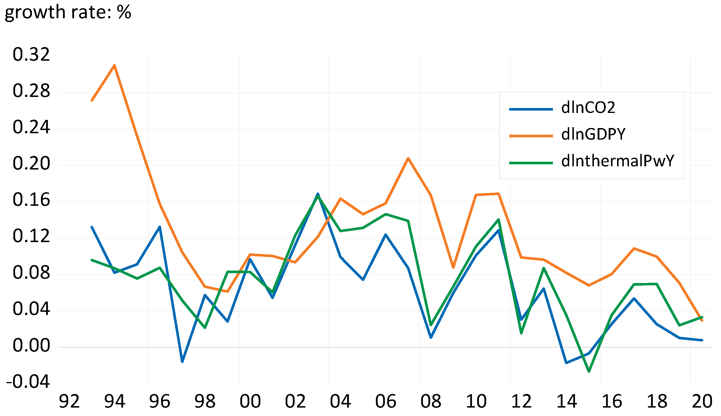
dlnCO2	Growth rate of CO2 emissions by the power industry	28	−0.01735	0.16883	0.06484	0.05032
dlnGDPY	Yearly GDP growth rate	28	0.02944	0.30999	0.12931	0.06559
dlnthermalPwY	Yearly growth rate of electricity from thermal power stations	28	−0.02669	0.16638	0.07719	0.04709
dlnGDPQ	Quarterly GDP growth rate	115	−0.010157	0.09889	0.03302	0.02301
dlnthermalPwM	Monthly growth rate of electricity from thermal power stations	347	−0.018903	0.18882	0.00668	0.04262

.

As a preliminary measure, in order to determine the relationship between carbon emissions and both GDP and thermal power, we put the annual data of carbon emissions, GDP, and thermal power in a graph, as shown in Figure 3 below. It can be seen that there is a similar trend among the three variables, and the correlation is relatively strong. At the same time, it shows that thermal power has a certain lead relative to carbon emissions, which encouraged us to make precise predictions.

The MIDAS model requires data to be a stationary time series, so a stable ADF test was conducted on the differentiated data. The results are shown in

Table 3. Stationary test results.

Symbol	ADF Testing	p-Value	Result
dlnCO2	−4.125755	0.0161	Stationary **
dlnGDPY	−1.810576	0.0674	Stationary *
dlnthermalPwY	−3.062216	0.0418	Stationary **
dlnGDPQ	−4.241424	0.0009	Stationary ***
dlnthermalPwM	−19.30022	0.0000	Stationary ***

Note: The symbols ***, **, and * represent significance at the significant levels of 1%, 5%, and 10%, respectively.

below. It can be seen that the data were stable.

5. Empirical Analysis

5.1. Model Estimation

In order to make comparisons and forecasts, we used a total of five models, which are as follows: the first model is the ARDL model using the annual GDP data to predict the carbon emissions of the power industry, the second model is the ARDL model using the annual power data to predict the carbon emissions of the power industry, the third model is the MIDAS model using quarterly GDP data to predict the annual carbon emissions of the power industry, the fourth model is the MIDAS model using the monthly data of thermal power to predict the annual carbon emissions of the power industry, and the fifth model is the multivariable MIDAS model used to predict the carbon emissions of the power industry by using the quarterly GDP data and the monthly thermal power data. As mentioned above, the RMSE, MAPE, and MASE were calculated to determine the best lag value of $k$. Models 1 to 5 were specificized as follows:

Model 1:

$${\mathrm{dlnCO}}_{2 t}={\beta }_0+{{\displaystyle \sum }}_{j=1}^q{\beta }_j{\mathrm{dlnCO}}_{2 t-1}+{{\displaystyle \sum }}_{i=0}^p{a}_i{\mathrm{dlnGDPY}}_{t-i}+u_t$$

(12)

Model 2:

$${\mathrm{dlnCO}}_{2 t}={\beta }_0+{{\displaystyle \sum }}_{j=1}^q{\beta }_j{\mathrm{dlnthermalPwY}}_{t-1}+{{\displaystyle \sum }}_{i=0}^p{a}_i\mathrm{dlnthermalPwY}+u_t$$

(13)

For the ARDL models, the lag order was automatically selected by the software.

Model 3:

$${\mathrm{dlnCO}}_{2 t}={\beta }_0+{\beta }_{1}B\left(L^{1/4};\theta \right){\mathrm{dlnGDPQ}}_t^{\left(4\right)}+{\epsilon }_t$$

(14)

Model 4:

$${\mathrm{dlnCO}}_{2 t}={\beta }_0+{\beta }_{2}B\left(L^{1/12};\theta \right){\mathrm{dlnthermalPwM}}_t^{\left(12\right)}+{\epsilon }_t$$

(15)

Model 5:

$${\mathrm{dlnCO}}_{2 t}={\beta }_0+{\beta }_{1}B\left(L^{1/4};\theta \right){\mathrm{dlnGDPQ}}_t^{\left(4\right)}+{\beta }_{2}B\left(L^{1/12};\theta \right){\mathrm{dlnthermalPwM}}_t^{\left(12\right)}+{\epsilon }_t$$

(16)

For MIDAS, the Almon polynomial was selected as the weight function, and the accuracy index was used to determine the optimal lag value $k$.

As can be seen from

Table 4. Accuracy indices of different models.

Model	1	2	3	4	5
	ARDL		MIDAS
Variable	dlnGDPY	dlnthermalPwY	dlnGDPQ	dlnthermalPwM	dlnGDPQ dlnthermalPwM
RMSE	0.050012	0.055784	0.041391	0.041428	0.037131
MAPE	286.7752	270.9444	259.2398	269.2595	197.0581
MAE	0.045379	0.04354	0.034088	0.03489	0.030401
Lag	ARDL(5,1)	ARDL(5,4)	K1 = 2	K2 = 18	K1 = 13, K2 = 26

, if the ARDL model was used for prediction, the RMSE values of annual GDP and annual power generation, as independent variables, were 0.05 and 0.056, respectively; accordingly, the best lag for these was found for ARDL (5,1) and ARDL (5,4). The RMSE of Model 1 was relatively lower than that of Model 2, indicating that using GDP is more accurate than using annual power. For the MIDAS model, the RMSE values of quarterly GDP and monthly power were 0.04139 and 0.0414, respectively, which are basically the same, but both are lower than those of the ARDL model, indicating that the MIDAS model had advantages in predicting annual CO₂ emissions. At the same time, for the multivariable model, that is, the model using both quarterly GDP and monthly power generation data, the RMSE reached the lowest level among the five models, indicating that the M(n)-MIDAS (m, K) model has the greatest advantage for predicting annual CO₂ emissions.

For each of the models, the evaluated results and the coefficient of the equation are shown in

Table 5. Coefficients of the models.

Variable	Models
	ARDL		MIDAS
	1	2	3	4	5
dlnCO2 (−1)	−0.491435 (0.357392)	−0.683536 ** (0.171498)	—	—
dlnGDPY	1.145907 ** (0.485071)	—	—	—
dlnGDPY (−1)	−0.444184 (0.407048)	—	—	—
dlnthermalPwY	—	0.581409 *** (0.071905)	—	—
dlnthermalPwY (−1)	—	0.691681 ** (0.168351)	—	—
dlnGDPQ	—	—	2.931045 ** (2.825309)	—	0.365510 (0.300701)
dlnthermalPwM	—	—		0.543143 *** (0.179435)	0.722755 ** (0.227343)
Intercept	0.117435 ** (0.040799)	0.08185 ** (0.012126)	0.027616 (0.022987)	0.025505 (0.017184)	0.008504 (0.033976)
AIC	−3.450208	−6.778780	−3.433334	−3.783747	−4.082098
R-squared	0.629634	0.991101	0.312447	0.515689	0.731822

Note: The symbols *** and **, represent significance at the levels of 1% and 5%, respectively.

.

If we compare Model 1 with Model 5, it can be seen that, both in the ARDL model and the MIDAS model, GDP and power had a positive effect on carbon dioxide emissions. From the perspective of the R-square value, Model 2 had the best simulation results, followed by Model 5 and Model 1, but the RMSE values of Model 1 and Model 2 were not the best. The R-square values of Model 3 and Model 4 are lower, indicating that the two models need other explanatory variables, and there may be a problem of variable omission, whereas the R-square of Model 5 is acceptable and the model has the lowest RMSE.

If we take all these points together, Model 5 is the optimal model among the five models, demonstrating that the carbon emissions of the power industry are related not only to thermal power generation but also to GDP, because power is closely related to economic development. At the same time, Model 5 is also able to make instant predictions, as it can predict the carbon dioxide emissions of the coming year in advance, based on the quarterly and monthly data disclosed within the year, without waiting for full disclosure of the annual data, which solves the data disclosure lag problem.

5.2. Nowcasting and Forecasting

At the time of writing, China’s monthly thermal power generation and quarterly GDP for 2021 have been fully announced, but the power industry’s 2021 carbon emissions have not been released. Based on the principle of the h-step models mentioned above, carbon emissions in 2021 can be estimated by using the GDP for the first, second, third, and fourth quarters of 2021, as well as monthly electricity production for the whole year. At the same time, carbon emissions in 2022 can be estimated by using the data for the whole year of 2021. The estimated results are as shown in

Table 6. Nowcasting and forecasting of carbon emissions of the power industry.

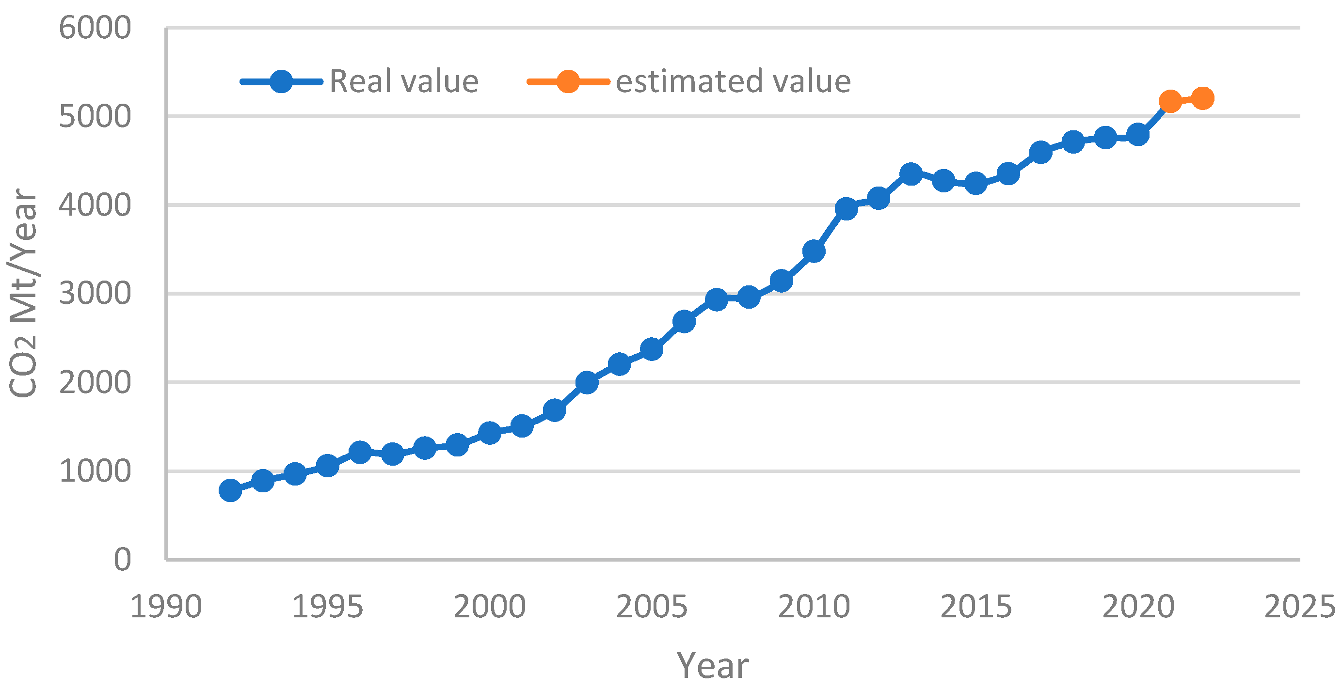
Steps	Year of 2021 (Mt CO2/Year)	Year of 2022 (Mt CO2/Year)
h = 0	5166.04	—
h = 1	5069.03	—
h = 2	5072.39	—
h = 3	5187.45	—
h = 4	5225.81	5201.84

.

As can be seen from Table 6, in forecasts of carbon emissions in 2021, according to the different h steps (from h = 0 to h = 4), the value of carbon emissions in 2021 has been revised quarterly, but are basically stable at around 5100 Mts. Among the different steps, when h = 0, the model uses all data from four quarters for GDP and 12 months of data on thermal power generation, so we chose 5166.04 Mt as the nowcasting value for the 2021 carbon emissions. Meanwhile, when h = 4, the model uses the data from last year to forecast the current year, so the 2022 carbon emissions are forecasted to be 5201.84 Mt. If the estimated values are included, we can construct a graph of China’s carbon emissions from 1992 to 2022, as shown in Figure 4.

According to Figure 4, the carbon emissions of China’s power industry have been and will still be maintaining a growth trend, despite the impact of COVID-19, which began in 2020; there was even a sharp increase in 2021 compared with 2020.

6. Conclusions

Applying the MIDAS model, in this study, we used data with different frequencies to build a framework for predicting carbon emissions from China’s power industry. When comparing MIDAS with a basic model, we found that the MIDAS model had a higher prediction accuracy than the ARDL model, and the MIDAS model with multiple independent variables had a higher prediction accuracy than the MIDAS models with single independent variables.

For the quarterly GDP and monthly thermal power generation data, we found that thermal power generation showed a strong correlation with the carbon emissions of the power industry, and had a certain leading predictive forecast ability, which could help governments to deeply explore the sources of carbon emissions and to implement the necessary policy to restrain thermal power or replace it with other kinds of energy.

The MIDAS model has the function of real-time prediction. This function allows the model to keep revising the forecast result with the latest data, which helps to establish a timelier carbon emission prediction system. In this study, we forecasted that the carbon emissions of China’s power industry in 2021 and 2022 will maintain an upward trend. This is mainly due to the fast economic recovery from the pandemic and the strong demand for energy in China in 2021. According to China’s National Bureau of Statistics, the total thermal power generation in 2021 has increased by 6.48% compared with 2020, whereas the GDP growth rate in 2021 was 8.1%, compared with the value of 2.2% in 2020. From a global perspective, carbon emissions are also likely to rebound, which was estimated by recent research [36].

In conclusion, by constructing a framework for forecasting carbon emissions in a single industry, this study suggests a new method that improves the accuracy and timeliness of forecasting and can be used to enrich the tools of carbon emissions forecasting. Especially for China, this prediction framework is useful for in-depth explorations of the sources of carbon emissions and for meeting the reduction goals as scheduled.

7. Discussion and Recommendations

For a long time, China’s electricity supply has been mainly based on coal-fired power plants, which not only drive up carbon emissions but also cause air pollution. In fact, the proportion of the installed capacity of coal power in Chinahas gradually decreased in recent years. As of the end of 2020, it accounted for 49.07%, which was lower than 50% for the first time [2] but was still relatively high. Especially when the carbon emissions of the power industry in other countries have shown a downward trend, the carbon emissions of China’s power industry continue to grow. China is striving to be a developed country in the first half of this century, while research shows that, in general, the more developed the country, the greater its carbon dioxide pollution [37]. Considering that China’s electricity demand is still likely to be very large in the recent future, measures urgently need to be applied to reduce it. In the future, carbon emissions from the power generation industry can be reduced in the following ways. First of all, it is necessary to develop new energy and renewable energy for power plants, such as hydropower, nuclear power, wind power, and other types of power plants. Secondly, it is necessary to carry out technological transformation of thermal power plants to improve their energy utilization efficiency.

From a longer-term perspective, to achieve the goal of carbon neutrality, in addition to reducing carbon emissions, it is vital to carry out the step of carbon absorption and carbon storage. Advances in technology and sustainability will provide more possibilities. Moreover, environmentally friendly sources of alternative energy for industry should be applied. For example, it could be helpful to increase forestry coverage or to cultivate specific plants such as bamboo to increase carbon absorption [38,39]. China has a vast land area and has great potential in this field. Alternatively, through carbon capture technology, carbon in the air can be captured and converted into raw materials for the manufacture of fertilizers or other chemicals [40].

References

- Crippa, M.; Guizzardi, D.; Solazzo, E.; Muntean, M.; Schaaf, E.; Monforti-Ferrario, F.; Banja, M.; Olivier, J.; Grassi, G.; Rossi, S.; et al. GHG Emissions of All World Countries, EUR 30831 EN; Publications Office of the European Union: Luxembourg, 2021; ISBN 978-92-76-41547-3. [CrossRef]
- National Bureau of Statistics of P.R. China. Available online: https://data.stats.gov.cn (accessed on 10 February 2022). (In Chinese)
- The State Council of China. China Releases White Paper on Climate Change Response, 28 October 2021. Available online: http://english.www.gov.cn/news/videos/202110/28/content_WS617a1072c6d0df57f98e4115.html (accessed on 10 February 2022).
- Ghysels, E.; Santa-Clara, P.; Valkanov, R. The MIDAS Touch: Mixed Data Sampling Regression Models. UCLA, Finance. 2004. Available online: https://escholarship.org/uc/item/9mf223rs (accessed on 10 February 2022).
- Giannone, D.; Reichlin, L.; Small, D. Nowcasting: The real-time informational content of macroeconomic data. J. Monet. Econ. 2008, 55, 665–676. [Google Scholar] [CrossRef]
- Fang, D.; Zhang, X.; Yu, Q.; Jin, T.C.; Tian, L. A novel method for carbon dioxide emission forecasting based on improved Gaussian processes regression. J. Clean. Prod. 2018, 173, 143–150. [Google Scholar] [CrossRef]
- Wu, L.; Liu, S.; Liu, D.; Fang, Z.; Xu, H. Modelling and forecasting CO2 emissions in the BRICS (Brazil, Russia, India, China, and South Africa) countries using a novel multi-variable grey model. Energy 2015, 79, 489–495. [Google Scholar] [CrossRef]
- Chang, H.; Sun, W.; Gu, X. Forecasting Energy CO2 Emissions Using a Quantum Harmony Search Algorithm-Based DMSFE Combination Model. Energies 2013, 6, 1456–1477. [Google Scholar] [CrossRef] [Green Version]
- Köne, A.Ç.; Büke, T. Forecasting of CO2 emissions from fuel combustion using trend analysis. Renew. Sustain. Energy Rev. 2010, 14, 2906–2915. [Google Scholar] [CrossRef]
- Zhao, X.; Han, M.; Ding, L.; Calin, A.C. Forecasting carbon dioxide emissions based on a hybrid of mixed data sampling regression model and back propagation neural network in the USA. Environ. Sci. Pollut. Res. 2017, 25, 2899–2910. [Google Scholar] [CrossRef]
- Hosseini, S.M.; Saifoddin, A.; Shirmohammadi, R.; Aslani, A. Forecasting of CO2 emissions in Iran based on time series and regression analysis. Energy Rep. 2019, 5, 619–631. [Google Scholar] [CrossRef]
- Fang, K.; Tang, Y.; Zhang, Q.; Song, J.; Wen, Q.; Sun, H.; Ji, C.; Xu, A. Will China peak its energy-related carbon emissions by 2030? Lessons from 30 Chinese provinces. Appl. Energy 2019, 255, 113852. [Google Scholar] [CrossRef]
- Li, M.; Wang, W.; De, G.; Ji, X.; Tan, Z. Forecasting Carbon Emissions Related to Energy Consumption in Beijing-Tianjin-Hebei Region Based on Grey Prediction Theory and Extreme Learning Machine Optimized by Support Vector Machine Algorithm. Energies 2018, 11, 2475. [Google Scholar] [CrossRef] [Green Version]
- Lin, B.; Long, H. Emissions reduction in China’s chemical industry—Based on LMDI. Renew. Sustain. Energy Rev. 2016, 53, 1348–1355. [Google Scholar] [CrossRef]
- Fatima, T.; Xia, E.; Cao, Z.; Khan, D.; Fan, J.-L. Decomposition analysis of energy-related CO2 emission in the industrial sector of China: Evidence from the LMDI approach. Environ. Sci. Pollut. Res. 2019, 26, 21736–21749. [Google Scholar] [CrossRef] [PubMed]
- Yang, H.; O’Connell, J.F. Short-term carbon emissions forecast for aviation industry in Shanghai. J. Clean. Prod. 2020, 275, 122734. [Google Scholar] [CrossRef]
- Zhang, S.; Wang, J.; Zheng, W. Decomposition Analysis of Energy-Related CO2 Emissions and Decoupling Status in China’s Logistics Industry. Sustainability 2018, 10, 1340. [Google Scholar] [CrossRef] [Green Version]
- Bahmani-Oskooee, M.; Chi Wing Ng, R. Long-Run Demand for Money in Hong Kong: An Application of the ARDL Model. Int. J. Bus. Econ. 2002, 1, 147–155. [Google Scholar]
- Ozturk, I.; Acaravci, A. The causal relationship between energy consumption and GDP in Albania, Bulgaria, Hungary and Romania: Evidence from ARDL bound testing approach. Appl. Energy 2010, 87, 1938–1943. [Google Scholar] [CrossRef]
- Chen, S. The Urbanization Impacts on the Policy Effects of the Carbon Tax in China. Sustainability 2021, 13, 6749. [Google Scholar] [CrossRef]
- Wang, Q.; Xiao, K.; Lu, Z. Does Economic Policy Uncertainty Affect CO2 Emissions? Empirical Evidence from the United States. Sustainability 2020, 12, 9108. [Google Scholar] [CrossRef]
- Foroni, C.; Marcellino, M.; Schumacher, C. Unrestricted mixed data sampling (MIDAS): MIDAS regressions with unrestricted lag polynomials. J. R. Stat. Soc. Ser. A Stat. Soc. 2013, 178, 57–82. [Google Scholar] [CrossRef]
- Ghysels, E.; Sinko, A.; Valkanov, R. MIDAS Regressions: Further Results and New Directions. Econ. Rev. 2007, 26, 53–90. [Google Scholar] [CrossRef]
- Galvão, A.B. Changes in predictive ability with mixed frequency data. Int. J. Forecast. 2013, 29, 395–410. [Google Scholar] [CrossRef] [Green Version]
- Guérin, P.; Marcellino, M. Markov-switching MIDAS models. J. Bus. Econ. Stat. 2013, 31, 45–56. [Google Scholar] [CrossRef] [Green Version]
- Breitung, J.; Roling, C. Forecasting inflation rates using daily data: A nonpara-metric MIDAS approach. J. Forecast. 2015, 34, 588–603. [Google Scholar] [CrossRef]
- Ghysels, E.; Santa-Clara, P.; Valkanov, R. Predicting volatility: Getting the most out of return data sampled at different frequencies. J. Econom. 2006, 131, 59–95. [Google Scholar] [CrossRef] [Green Version]
- Forsberg, L.; Ghysels, E. Why Do Absolute Returns Predict Volatility So Well? J. Financ. Econom. 2007, 5, 31–67. [Google Scholar] [CrossRef]
- Alper, C.E.; Fendoglu, S.; Burak, S. Forecasting Stock Market Volatilities Using MIDAS Regressions: An Application to the Emerging Markets. Munich Pers. RePEc Arch. 2008, 7460. Available online: https://mpra.ub.uni-muenchen.de/7460/ (accessed on 10 February 2022).
- Körs, M.; Karan, M.B. Stock exchange volatility forecasting under market stress with MIDAS regression. Int. J. Finance Econ. 2021, 1–12. [Google Scholar] [CrossRef]
- Kuzin, V.; Marcellino, M.; Schumacher, C. MIDAS vs. mixed-frequency VAR: Nowcasting GDP in the euro area. Int. J. Forecast. 2011, 27, 529–542. [Google Scholar] [CrossRef] [Green Version]
- Pan, Z.; Wang, Q.; Wang, Y.; Yang, L. Forecasting U.S. real GDP using oil prices: A time-varying parameter MIDAS model. Energy Econ. 2018, 72, 177–187. [Google Scholar] [CrossRef]
- Li, X.; Shang, W.; Wang, S.; Ma, J. A MIDAS modelling framework for Chinese inflation index forecast incorporating Google search data. Electron. Commer. Res. Appl. 2015, 14, 112–125. [Google Scholar] [CrossRef]
- Gunay, S.; Can, G.; Ocak, M. Forecast of China’s economic growth during the COVID-19 pandemic: A MIDAS regression analysis. J. Chin. Econ. Foreign Trade Stud. 2020, 14, 3–17. [Google Scholar] [CrossRef]
- Chevallier, J. COVID-19 Outbreak and CO2 Emissions: Macro-Financial Linkages. J. Risk Financ. Manag. 2020, 14, 12. [Google Scholar] [CrossRef]
- Friedlingstein, P.; Jones, M.W.; O’Sullivan, M.; Andrew, R.M.; Bakker, D.C.E.; Hauck, J.; Le Quéré, C.; Peters, G.P.; Peters, W.; Pongratz, J.; et al. Global Carbon Budget 2021. Earth Syst. Sci. Data Discuss. 2021, 1–191. [Google Scholar] [CrossRef]
- Borowski, P.F. Significance and Directions of Energy Development in African Countries. Energies 2021, 14, 4479. [Google Scholar] [CrossRef]
- Borowski, P.F.; Patuk, I.; Bandala, E.R. Innovative Industrial Use of Bamboo as Key “Green” Material. Sustainability 2022, 14, 1955. [Google Scholar] [CrossRef]
- Mitchell, C.D.; Harper, R.J.; Keenan, R.J. Current status and future prospects for carbon forestry in Australia. Aust. For. 2012, 75, 200–212. [Google Scholar] [CrossRef]
- Liu, H.; Gallagher, K.S. Catalyzing strategic transformation to a low-carbon economy: A CCS roadmap for China. Energy Policy 2010, 38, 59–74. [Google Scholar] [CrossRef]