Abstract
The contribution of litterfall (dead leaves, twigs, etc., fallen to the ground) and forest floor (organic residues such as leaves, twigs, etc., in various stages of decomposition, on the top of the mineral soil) is fundamental in both forest ecosystem sustainability and soil greenhouse gases (GHG) exchange system with the atmosphere. The effect of different thinning treatments (control-no thinning, traditional-low thinning, selective-intense thinning) on litterfall and forest floor nutrients, in relation to soil GHG fluxes, is analyzed. After one year of operations, thinning had a significant seasonal effect on both litterfall and forest floor, and on their nutrient concentrations. The intense (selective) thinning significantly affected the total litterfall production and conifer fractions, reducing them by 46% and 48%, respectively, compared with the control (no thinning) sites. In the forest floor, thinning was able to significantly increase the Fe concentration intraditional thinning by 59%, and Zn concentration in the intense thinning by 55% (compared with control). Overall, litterfall acted as a bio-filter of the gasses emitting from the forest floor, acting as a GHG regulator.
1. Introduction
In a climate change context, forest ecosystems play a key role due to the removal of anthropogenic CO2 emissions from the atmosphere and their sequestration as carbon [1]. Forest can store carbon in different pools such as living biomass, root system, dead wood, litter, organic and mineral soil [2,3,4]. It is estimated that half of the Earth’s terrestrial carbon is stored in forests and about 70% of it is sequestered to soil [5,6]. Due to the high dynamic of forest ecosystems, the adoption of reduction and mitigation targets in the forest sector was one of the principles of the Kyoto Protocol as part of a broader climate change platform [7]. In this sense, the implementation of forest management practices, such as thinning [5,8], affect the rate of carbon accumulation in the forest ecosystem due to changes in aboveground live biomass, the soil properties such as aggregate formation, the water content, the soil pH and thus the net ecosystem productivity (NEP). In general, NEP represents the sum of changes of these pools and any alteration of them due to implementation of forest sustainable practices affects the NEP balance [9].
Litterfall production also plays a primary role in both the forest ecosystem’s sustainability [10,11] and in the greenhouse gases (GHG), hereinafter referred to as the GHG exchange system (CO2, CH4, N2O), which occurs between the soil and the atmosphere [12,13]. Any alteration in the soil’s litter layer can influence the soil’s GHG seasonal variation [14].
Plant litter is transformed into soil organic matter through decomposition, thus releasing CO2 into the atmosphere. The decomposition of the forest litter results in the formation of humic substrates. The microbial communities, along with fungi and other soil biota, are responsible for the process. The mechanism for the formation of soil humic molecules is still unclear, with many describing them as macromolecules [15]) or supramolecular formations of smaller molecules [16] or a combination of both [17]. The soil humic environment and its microbial and fungal communities further degrade the organic molecules. Litter decomposition, in combination with other mechanisms driven by belowground soil processes (particularly root decomposition and rhizosphere activity), constitute the dominant mechanism of CO2 efflux from forest soil [18], which contribute a great amount to the total soil CO2 efflux [19].
Thinning as a forest management practice results in, among others, an increase in biomass productivity of any remaining trees and in a decrease in litterfall production and thus in nutrient inputs to the soil, immediately following thinning [20]. However, this litterfall reduction may reappear in the years following thinning operations [20,21].
Furthermore, the microenvironment altered by thinning may increase the decomposition of the litter and its transformation into soil organic matter, through a change of the nutrient mineralization [10]. Thinning also influences site productivity and the homogeneity of understory vegetation that causes seasonal and annual alteration of nutrients, changes to the initial litterfall decomposition rate and to seasonal and annual litterfall fluxes. These changes are driven by possible changes in the amount of leaves or needles falling to the ground, due to the reduction of competition among trees [22], as well as by micro-environmental changes [23]. It will also invariably affect the overall production of litterfall, particularly needle fall, twigs, and woody fractions [24].
The intensity of thinning has an impact on annual litterfall production in coniferous forests. It has been estimated that intense thinning reduces annual litterfall, needles, and twigs fractions [22], and tends to reduce microbial C and nitrogen (N) pools as well as soil net CO2 efflux. On the other hand, intense thinning also results in stand density reduction and accelerates nutrient release from decomposing needles due to high water availability and, therefore, results in a higher nutrient availability [11]. Thus, both litterfall production and the nutrient release through litter decomposition, combined with the applied silvicultural treatments, significantly affect the sustainability of the forest ecosystems [11].
Since the late 20th century, lack of planned management practices has led to the degradation of most of the coniferous plantation forests used for land restoration in the Mediterranean region [25]. Conifer plantations, due to lack of planned management, show reduced density, reduced productivity and resilience capacity, and accumulation of deadwood [26].
In a degraded forest, the lack of proper management practices can affect the C sequestration rate, reducing the sink potential of these forests [25]. It is estimated that the soil’s carbon concentration is higher in forests without silvicultural treatment, showing a trend to augment soil carbon sequestration [10]. Furthermore, the absence of proper silvicultural practices in combination with regional climate conditions (warm and dry summer and mild rainfall in winter) affect the soil GHG exchange system to the atmosphere. For example, the creation of anaerobic conditions in the soil leads to CH4 production [25,27], while altered seasonal soil environmental factors (mainly temperature and moisture) affect the microbial processes and therefore the rate of N2O production [28].
Litter decomposition and the nutrients in the biochemical cycle of organic matter [23], i.e., the movement and transformation of chemical elements within or among the biotic and abiotic components of the soil, as a result of biological, mechanical, and chemical processes, and the effect of thinning on litter decomposition dynamics and GHG fluxes [11,22], play a key role in the function and stability of forest ecosystems. Therefore, their study is essential especially in the Mediterranean region where data are lacking. In Greece, in particular, most of the peri-urban conifer forests are degraded due to the lack of sustainable management practices [29], and there is limited knowledge of thinning effects on forest mass and litterfall production or their correlation to soil atmosphere GHG fluxes exchange.
Thinning is expected to affect the litterfall and forest floor, thus affecting the nutrient inputs to the soil. Thinning is also expected to affect the soil GHG fluxes. The aim of this study wasto test these hypotheses, and specifically: (i) to quantify the seasonal and thinning effect of different thinning treatments (control-no thinning, traditional-low thinning, selective-intense thinning) on the litterfall and forest floor nutrients; (ii) to investigate the effect of thinning on litterfall production; and (iii) to assess the relationship between litterfall production and nutrient release with soil GHG fluxes, after one year of thinning interventions, in a degraded coniferous forest in Greece.
2. Materials and Methods
2.1. Study Site
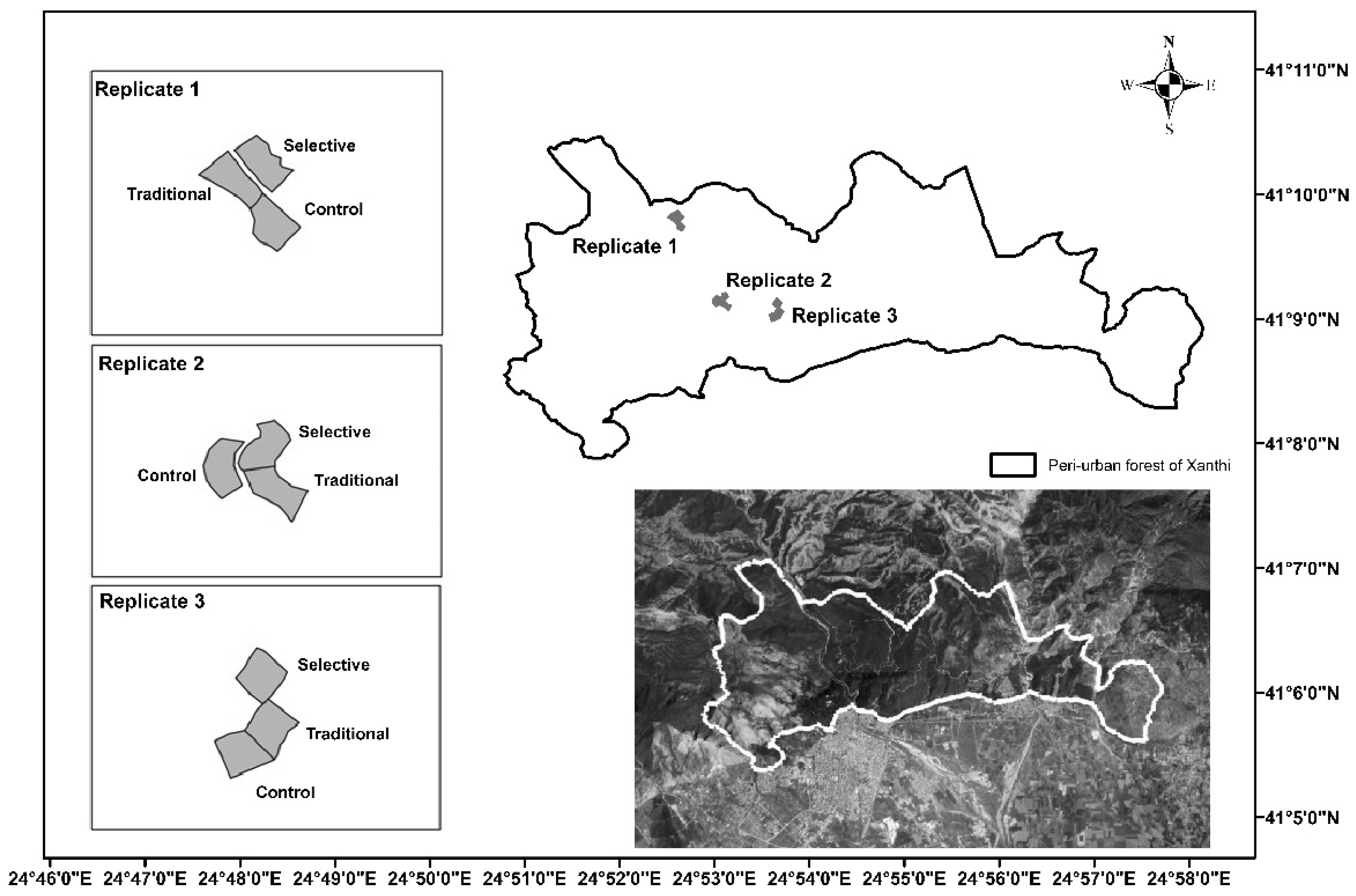
The study site is located at the peri-urban forest of Xanthi (41°9′27.3″ N–24°54′9.8″ E, Greece) that covers an area of approximately 2400 ha and is a part of the Xanthi–Gerakas–Kimerion public forest (Figure 1). The management of the state forest is based on a ten-year plan by Xanthi’s Forest Service; however, lack of sustainable timber production and overgrazing has led to forest degradation [30]. The prevailing attribute of the study site is, among other things, the large range of slopes found in the forest landscape that reach inclines of up to 80%. The soil type is Cambisols [31] with a moderately acidic pH (5.6), loam texture, and a high percentage of sand that goes up to about 60% [32]. The soil organic C is low, compared to more humic soils (62 Mg·ha−1), and the soil water content (SWC) is 15% (annual average). The plantations began in the 1940s with most of them established by the mid-1970s [30], with Calabrian pine (Pinus brutia Ten) being the dominant species, whereas Maritime pine (Pinus maritima Mill), Black locust (Robinia pseudoacacia L.), Mediterranean cypress (Cupressus sempervirens L.) and Austrian pine (Pinus nigra J.F. Arnold) were secondary [33]. Under the overstory, broadleaf tree species such as the Kermes oak (Quercus coccifera L.), South European flowering ash (Fraxinus ornus L.), Oriental hornbeam (Carpinus orientalis L.), Hungarian oak (Quercus frainetto Ten), Sessile oak (Quercus petraea Liebl. subsp. polycarpa (Schur) Soo), Pubescent oak (Quercus pubescens Willd), etc., have been naturally established [34]. The area’s climate is characterized as semi-wet to dry, with rainy winters and dry summers [30]. The annual mean temperature and precipitation is 15.5 °C and 675 mm, respectively [35]. The mean total height of the conifers at the study site prior to thinning was 19.74 m, with a mean stand volume of the standing trees 0.74 m3 per tree and 315.54 m3/ha [32]. The deadwood volume at the study site was 9.21 m3·ha−1 [36].

Figure 1.
Shape and location of the study site. Peri-urban forest is marked with thick white solid line (Xanthi Forest Directorate).
2.2. Thinning Treatments
At the study site, three replicates for each thinning treatment (control-no thinning, traditional-low thinning, selective-intense thinning) were applied uniformly (Figure 1). In each replicate two monitoring circular plots (radius 13 m and area 531 m2) were established for each treatment. The design of the three different thinning approaches is that of the LIFE FORESMIT research project, in which the objective was to study the effects of different thinning implementation in the climate change mitigation context [25]. For the present study, measurements were carried out in one of the two monitoring plots of each replicate, i.e., in a total of nine plots.
Traditional thinning is the silvicultural intervention that was applied in the peri-urban forest of Xanthi up to the present time by the Forest Service. Selective thinning was applied to quickly transform the peri-urban forest into a forest of broadleaf species, at least in more productive sites [34].
In traditional thinning the dead, damaged, malformed, suppressed and intermediate trees are cut in the overstory. The intensity of the treatments depends on the overstory pine tree density. In the lower stories, thinning is aimed at a uniform distribution of broadleaves, and in most cases, the trees having good form as well as the robust trees are not cut [34]. In selective thinning, the main objective in the overstory is to release broadleaf trees of the lower stories. In the cuttings of the overstory, the dead, damaged and badly formed trees are cut. As a priority, the trees with large dimension and bad form are removed (if there is an adequate ground coverage by broadleaf trees or broadleaf tree regeneration), while the trees with the best form are not cut. However, where the cutting of the trees with bad form (or damaged trees) is not adequate for the release of a group of broadleaf trees and there is a need for the cutting of a tree having the best form, then that tree is cut. The intensity of the thinning–cutting depends on the density of the broadleaves and the need for their release and on the density of the overstory pines. When dense or rather dense groups of broadleaf trees covered the ground totally, then all the overstory trees are removed in one silvicultural application (cutting) if serious damage to broadleaf trees can be avoided [34]. In the lower stories, the thinning of broadleaf trees is done as a type of “positive selection” thinning. Based on positive selection, the main competitor for each of the best selected broadleaved trees (strong growth vigor, symmetric and large crown) is removed [34]. In the control plots, no silvicultural intervention took place. The duration of all thinning operations was one month (September 2016). The cut trees were separated into trunks, branches and leaves-needles. Branches and leaves-needles were chipped with a small-sized machine, and they were uniformly distributed in the stands. Trunks were moved to the nearest forest roads and were offered to the local population for their domestic needs, according to the national legislation regarding thinning operations (Presidential Decree no 86/1969).
The selective thinning approach was more intense compared to its traditional counterpart. In the traditional thinning the total basal area was reduced from 38.96 m2·ha−1 to 30.93 m2·ha−1, while in the selective thinning, the total basal area was reduced from 39.27 m2·ha−1 to 23.81 m2·ha−1 [34].
2.3. Litterfall and Forest Floor Collection
Litterfall consisted of dead leaves, twigs etc., collected from above ground traps, which were set for the estimation and evaluation of the litter decomposition and nutrient dynamics [10,24,37]. Particularly, within each of the nine plots, two traps (50 × 50 × 30 cm) were randomly placed 1 m from the ground, amounting to a total of 18 traps. The traps set near the collars were used for the measurement of soil GHG fluxes [32].
The trapped litter was collected once at the end of each season (autumn, winter, spring, summer) on a similar date between samplings. The sample collections were made on the same day with GHG measurements. The litter was collected from the traps in numbered paper bags. On each sampling day, 18 bags of samples were collected from the nine plots. Each litterfall sample was separated in eight different fractions (four for conifers and four for deciduous trees) and carefully placed in labelled paper bags; pine needles, deciduous leaves, twigs and branches <4.5 cm, reproductive structures and bark. Based on the litter sample collected from each trap, the total number of the labelled paper bags, each consisting of the separating fraction, reached a maximum of 144 at each sampling day. In total, at the end of the study period the collected litter was sorted in 1122 labelled paper bags. After the assortment, the labelled paper bags were dried in a forced-air oven for at least 48 h at 80 °C (dried to constant weight) at the laboratory and weighed for biomass evaluation.
The forest floor consists of litterfall and herbaceous vegetation, which was scraped from the ground up to a depth of 10 cm. Here we should clarify that the maximum depth of the scraped soil was 10 cm and that the topsoil depth varied significantly within the study area. Eighteen (18) forest floor samples were collected four times (October, January, March, June) with the use of a 25 × 25 cm metal frame at the same dates as the sampling from the litter boxes. Timing of the measurements was chosen empirically, in order to cover the expected seasonal variation. Both the litter and the forest floor samples were dried at 80 °C in an oven for 48 h and then their dry weight was measured. The samples were milled in order to make the analysis of total nitrogen content, in both litter and floor samples, by the Kjeldahl method [38]. The K, Ca, Mg, Na, Fe, Mn, Cu, and Zn content were estimated after dry ashing. The ash was washed with a 5 mL solution made up of a 6 N HCl solution, and in the final solution, the nutrient elements were measured in an ICP OES Optima 8300 (PerkinElmer, Inc., Waltham, MA, USA). The Fe, Cu, Mn, and Zn content were measured at 238.204 nm, 327.393 nm, 257.61 nm and 206.2 nm, respectively. On the other hand, the P, K, Ca and Mg were evaluated at 1:10 dilution at 213.617 nm, 766.49 nm, 317.933 nm and 285.213 nm, respectively. The dilution was essential to achieve accuracy at the macro element measurement [39].
2.4. Methodology of GHG Fluxes
The static closed chamber method was used for the measurements of soil GHG fluxes. This method is widely used in studies of the soil GHG exchange system with the atmosphere, especially in field experiments under the piloting of different treatments [40]. Gas sampling was undertaken in each of the nine plots at bimonthly intervals from October 2016 to September 2017. Two chamber collars (30 cm in diameter) were installed, at a minimum of 5 cm depth, into the soil in each plot, in September 2016. During each gas sampling event, both chambers in each plot were closed for 30 min and gas samples were collected four times at intervals of 0, 10, 20 and 30 min after closing the chambers. At each sampling time, 8 gas samples were collected from each plot, 72 samples in total [32]. The gas was collected with a plastic syringe of 30 mL with a 22 G 0.7 × 25.4 mm hypothermic needle inserted through the septum. After pushing 5 mLof gas out of the syringe, 25 mLwas transferred immediately in pre-evacuated 12 mL glass exetainer vials (Labco Limited, Lampeter, UK). The GHG samples were sent to the laboratory of the Research Centre for Agrobiology and Pedology in Florence, Italy, and were analyzed within 4 weeks after collection using a GC-2014 (Shimadzu Inc., Kyoto, Japan) gas chromatograph [41].
Fluxes were estimated using the linear slope of gas concentration versus chamber closure time and enclosed soil surface area, using the following linear equation:
where:
Flux rate F = V∗(dC)/A∗(dt)
- F = gas flux rate, mg·m−2·min−1
- V = volume of headspace, m3
- A = area covered of static chamber, m2
- dC = change in gas concentration, mg·m−3
- dC = gas concentration at time t3 − gas concentration at time t1
- dt = change in time, min
- dt = time t2 − time t1
Fluxes were set to zero if the change in gas concentration during chamber enclosure was below the minimum detection limit determined from the GC, and values were rejected if they passed the detection test but had an R2 < 0.75; in this case, fluxes were treated as missing data [25].
2.5. Statistical Analysis
All statistical analyses and graphics were performed using the SPSS statistical software [42] and R programing language [43]. SPSS was used for repeated measures ANOVA, with Greenhouse–Geisser correction to test the significant differences in both litterfall and forest floor production at each period (season) among thinning treatments. To ascertain the sphericity assumptions (p > 0.05), the Mauchly’s Test of Sphericity was used. An ANOVA was performed in order to estimate the effect size of both treatment and season on litterfall production. A Pearson correlation analysis, with p = 0.005 significance level, was used to detect possible correlations among forest floor, litterfall production and their nutrients released with GHG fluxes. Finally, post hoc Bonferroni tests were used to verify which treatments and seasons differed. The R package “vegan” [44] was used for principal component analysis (PCA) for exploring the correlation among the different nutrient concentrations (N, P, K, Ca, Mg Fe Mn, Zn) and GHG fluxes (CO2, CH4, N2O) that are responsible for the patterns seen among observations (seasons). We would like to know which nutrient concentrations and fluxes were influential, and how they were correlated. The “ggbiplot” package [45] was used for producing the PCA graphs.
3. Results
3.1. Seasonal and Thinning Effect on Forest Floor Nutrients
A significant seasonal effect was observed on all nutrients throughout the study (F (3, 32) = 10.96, p < 0.001). A post hoc test using the Bonferroni correction showed that the total concentration of nutrients was significantly higher during summer compared to autumn (p = 0.046) and winter (p < 0.001) but was not higher compared to spring (p = 0.870). The nutrients Mg, Mn, Ca, Cu and Fe had higher values in autumn compared to the rest of the seasons, whereas Zn presented higher values in spring and N in summer (Table 1). An increase of P, Mg, Mn and Z was observed in selective thinning across all seasons but was not deemed to be of significant value (p > 0.05) (Table 1).

Table 1.
Mean seasonal forest floor nutrients concentration (mean ± SD) expressed as mg·kg−1 of three replicates for three thinning treatments in period (16 October until 17 September). (C: Control, T: Traditional. S: Selective. N: Nitrogen, P: Phosphate, K: Potassium, Ca: Calcium, Mg: Magnesium, Cu: Copper, Fe: Iron, Mn: Manganese, Zn: Zinc).
Overall, thinning was observed to have a significant effect on nutrients (F (18, 32) = 7.497, p < 0.001). A post hoc test using the Bonferroni correction showed that, throughout the study period, the total concentration of Fe was found to be significantly higher in traditional thinning compared to the control (p = 0.004) at about 59% and compared to selective thinning (p = 0.003) at about 61%, whereas Zn was higher in selective thinning by 55% compared to traditional thinning (p = 0.048), but not to the control (p = 0.566).
Thinning was also observed to affect nutrients among seasons significantly (F (9, 21) = 6222, p < 0.001). In spring, P concentration was significantly reduced in traditional thinning compared to selective thinning (p = 0.047) and the control (p = 0.026). In spring N increased significantly in the traditional site compared to the selective (p = 0.041), but not to the control (p = 0.545), and K was increased in the control compared to the traditional site (p = 0.012). At the same season, comparing the two thinned sites, the mean concentrations of K and Mn were significantly increased in selective thinning compared to traditional thinning (p = 0.018 and p = 0.019, respectively) and showed a slight but not significant reduction when compared to the control (p = 0.681 and p = 0.846 respectively). Regarding Fe, a significant increase was observed in traditional thinning over selective thinning in all seasons except spring where the concentration was higher in the selective site (p = 0.989). Particularly during summer, Fe concentration in traditional thinning was higher compared to selective thinning (p = 0.031) and a slight, but insignificant, increase was observed over the control (p = 0.072). In both autumn and winter, Fe was also higher in traditional compared to both sites (selective p= 0.009 and control p = 0.006 and selective p = 0.026 and control p = 0.017, respectively). Differences among thinning treatments were detected in the remaining nutrients but were not deemed significant (Table 1).
3.2. Seasonal and Thinning Effect on Litterfall Nutrients
A significant effect of season on all nutrients was observed throughout the duration of the study (F (27, 41) = 6.44, p < 0.001). In particular, the concentrations of all nutrients were significantly higher in autumn (F (11, 3) = 20.55, p < 0.001) than in the rest of the seasons. Most nutrients (N, P, K, Mg, Mn and Zn) had higher values in spring when compared to winter and summer but these differences were non-significant (p > 0.05) (Table 2). A reduction of litterfall nutrient concentrations was observed in selective thinning for most of the litterfall nutrients throughout each season; however, no values were found to be significant (p > 0.05) (Table 2).
Table 2.
Mean seasonal litterfall nutrient concentrations (mean ± SD) expressed as mg·kg−1 of three replicates for three thinning treatments in the period (16 October to 17 September). (C: Control, T: Traditional. S: Selective. N: Nitrogen, P: Phosphate, K: Potassium, Ca: Calcium, Mg: Magnesium, Cu: Copper, Fe: Iron, Mn: Manganese, Zn: Zink).
3.3. Thinning Effect on Litterfall Production
One year after thinning (October 2016–September 2017), the treatment showed a significant effect on litterfall production (F (1.90, 20.90) = 5.98, p = 0.010). A post hoc test using the Bonferroni correction showed that the mean litterfall production was significantly higher at the control site (p = 0.032) than at the plots of selective thinning by about 46%, but was not significantly higher when compared to traditional thinning (p = 0.99). The lowest total cumulative litterfall production observed was in selective thinning, ranking last in the following order: control > traditional > selective (Table 3).
Table 3.
Mean cumulative litterfall production for each fraction and total (mean ± SD) expressed as kg·ha−1 of three replicates for three thinning treatments during four seasons in the study period (16 October until 17 September) (C: Control, T: Traditional. S: Selective, PN: pine needles, DL: deciduous leaves, PT: pine twigs, DT: deciduous twigs, PR: pine reproductive, DR: deciduous reproductive, PB: pine bark).
Significant differences of conifer fractions occurred among treatments (F (1, 11) = 10.44, p = 0.08) one year after thinning (Table 4). In particular, thinning was able to reduce conifer fractions significantly in selective thinning, by about 48%, when compared to controls (p = 0.00), whereas an increase of less than 20% was observed in deciduous subjects, but it was not found to be significant (p = 0.621) (Table 4). No data for deciduous bark were conclusive throughout the study period, presumably due to the very thin bark of the deciduous species caused by their young age.
Table 4.
Mean cumulative litterfall production for conifers and deciduous trees (mean ± SD) expressed as kg·ha−1 of three replicates for three thinning treatments during four seasons in the study period (16 October until 17 September). (C: Control, T: Traditional. S: Selective).
The mean annual cumulative pine needle litterfall from all treatments was 3063.52 ± 878.03 kg ha−1. Thinning was able to significantly affect pine needles production (F (1.87, 20.66) = 6.64, p = 0.008). A post hoc test using the Bonferroni correction showed that the mean pine needle fall production was significantly lower for selective thinning (p = 0.047) when compared to controls, and to traditional thinning (p = 0.042) kg ha−1. The mean cumulative production was ranked in the following order: control > traditional > selective (Table 3).
Thinning was able to significantly affect pine bark fractions (F (1.57, 17.30) = 4.34, p = 0.037), although this effect was lower than that of pine needles, with the mean annual cumulative litterfall reaching 811.31 kg ha−1 (Table 3). The mean cumulative production ranked in the following order: control > traditional > selective. The differences among the rest of litterfall fractions were found to be non-significant. Additionally, pine needles and pine bark followed a clear seasonal pattern throughout the study period for each of the three treatments. The maximum peaks for pine needles and pine bark occurred during the summer of 2017 (Figure 2a,g).
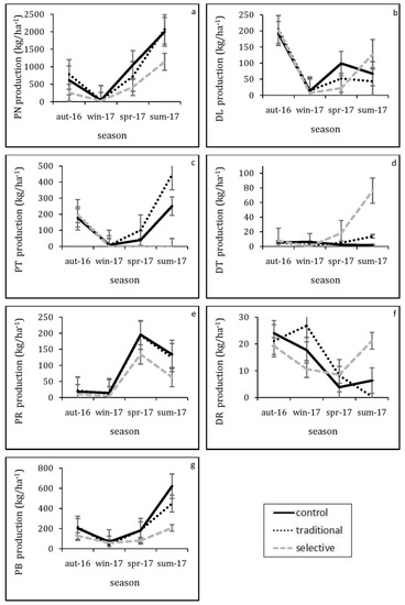
Figure 2.
Seasonal pattern (aut: autumn, win: winter, spr: spring, sum: summer) of litterfall fractions over the study period (16 October until 17 September). (a) PN pine needles, (b) DL deciduous leaves, (c) PT pine twigs, (d) DT deciduous twigs, (e) PR pine reproductive, (f) DR deciduous reproductive, (g) PB pine bark. Each data point represents the mean of the three replicates for each treatment (Control, Traditional and Selective). Error bars indicate the standard error.
3.4. Relationship between GHG Fluxes and Litterfall Production
During the study, the CH4 fluxes were always found negative, indicating a CH4 uptake throughout the study period. After a short-term period (six months) of thinning, the CH4 uptake was significantly negatively correlated with pine needles (p = 0.040) and pine bark (p = 0.006) (Table 5). After one year of thinning, the CH4 uptake variation was strongly negatively correlated to both pine twigs (p = 0.007) and pine bark (p = 0.020), but positively correlated to deciduous twigs (p = 0.019). On the other hand, CO2 fluxes were positively correlated to deciduous leaf (p = 0.039). Overall, the CH4 uptake was strongly and negatively correlated to total litterfall production (p = 0.040) (Table 5).
Table 5.
Pearson correlation analysis among GHG fluxes and litterfall fractions in two different periods, where r: correlation coefficient, p value: significance level, year−0.5: 6 months after thinning, year−1: 16 October until 17 September, PN: pine needles, DL: deciduous leaves, PT: pine twigs, DT: deciduous twigs, PR: pine reproductive, DR: deciduous reproductive, PB: pine bark, TL: total litterfall.
3.5. Forest Floor Nutrients and Soil GHG Fluxes
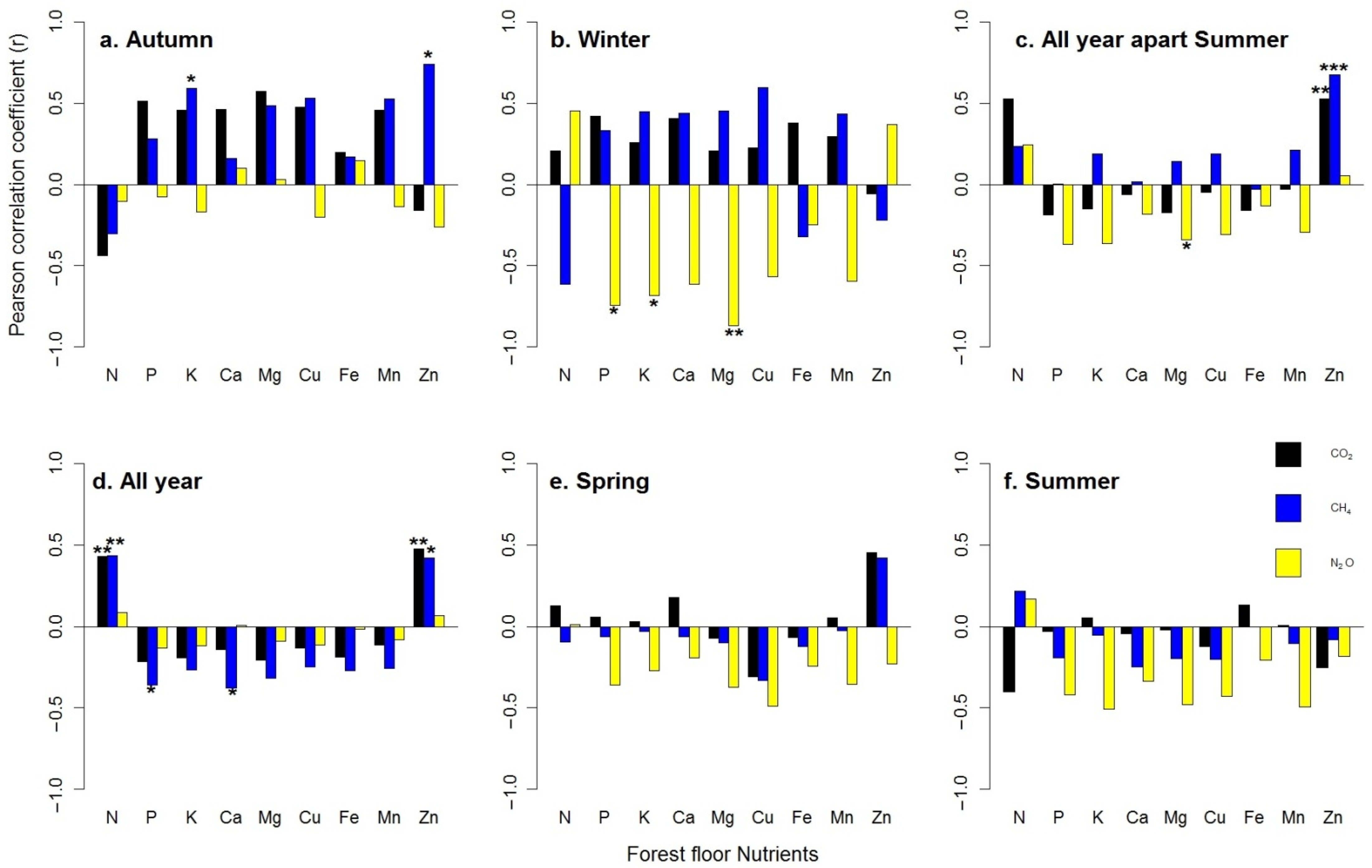
GHG fluxes and forest floor nutrients showed different patterns over the studied periods. In autumn, the CH4 uptake was positively correlated to Zn (Pearson’s r = 0.74 *) and K (r = 0.59 *) (Figure 3a), whereas in winter, the N2O fluxes were negatively correlated to P (r = −0.74 *), K (r = −0.68 *) and Mg (r = −0.87 **) (Figure 3b). Throughout the study period, except for the summer season, both CO2 and CH4 uptake variation were positively correlated with Zn (r = 0.53 ** and 0.67 ***), whereas N2O variation was negatively correlated with Mg (r = −0.34 *) (Figure 3c). In total, one year after thinning, Pearson correlation analysis showed that the CO2 fluxes were significant and positively correlated to N (r = 0.43 **) and Zn (r = 0.47 **) concentration, whereas the CH4 uptake was affected negatively by P (r = −0.36 *) and Ca (r = −0.38 *) and positively by N (r = 0.43 **) and Zn (r = 0.42 *). No significant relationships were detected among N2O and forest floor nutrients release (Table 6 and Figure 3d). No significant relationships were detected during spring and summer (Figure 3e,f).

Figure 3.
Seasonal pattern ((a) autumn, (b) winter, (c) all year apart from summer, (d) all year, (e) spring, (f) summer) of forest floor nutrients’ correlation with GHG fluxes over the study period (16 October until 17 September). Asterisks represent significance levels, accordingly: * = 0.05, ** = 0.01, *** = 0.001. Each bar represents the mean of the three replicates for each treatment (Control, Traditional and Selective).
Table 6.
Pearson correlation analysis among GHG fluxes and forest floor nutrients, one year after thinning, where r: correlation coefficient, p value: significance level.
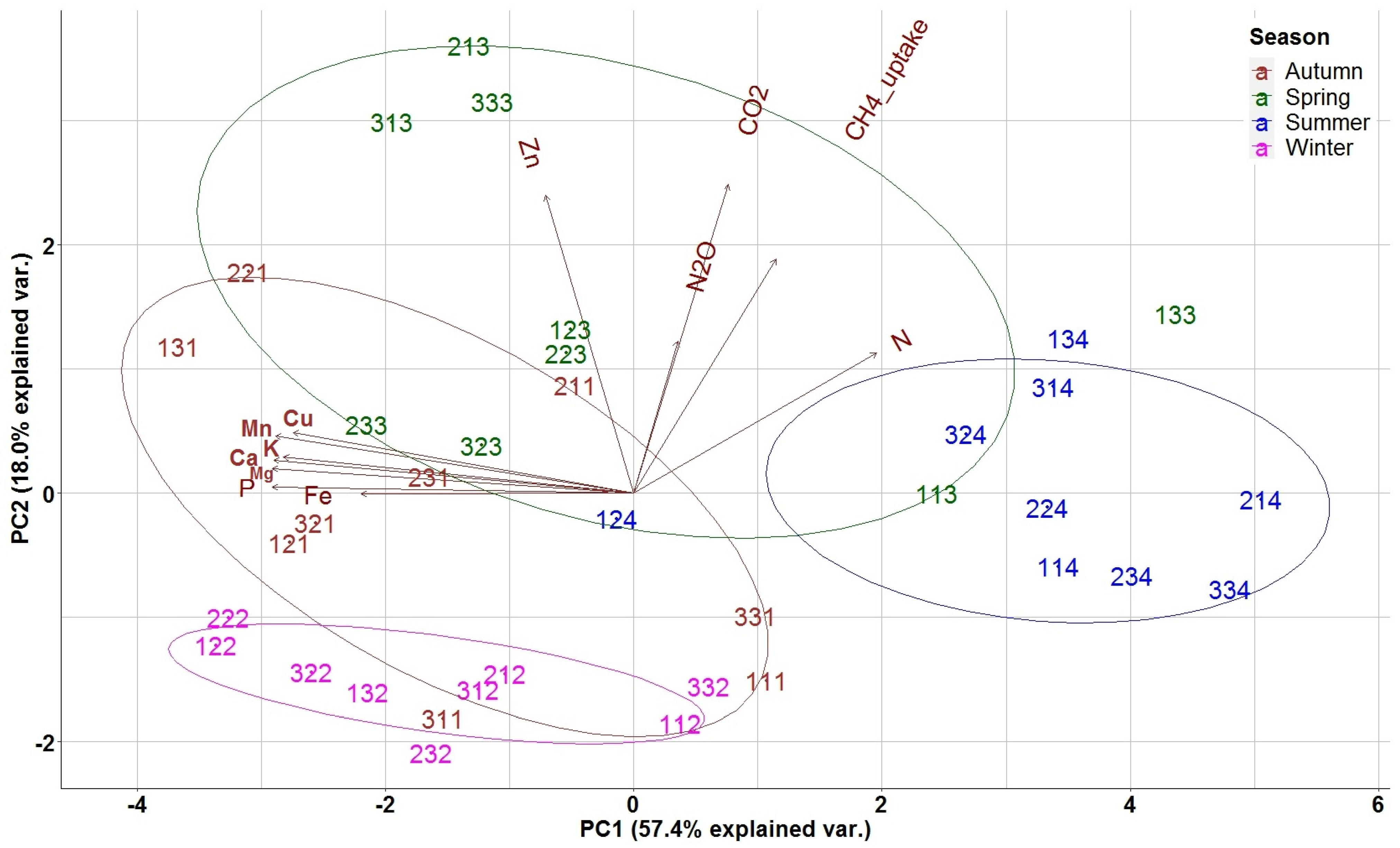
In the biplot of PCA analysis, the weights of the different variables are presented as arrows and vary by distance from the origin. The biplot enabled the evaluation of the correlation level among the quantified variables, with lines pointing in the same direction indicating closer correlation (Figure 4). A first group of variables (nutrients) including Fe, P, Mg, Mn, Ca and Cu, was very close and highly correlated. A second group including CO2, N2O, and the CH4 uptake (GHG fluxes) and to a lesser extent N and Zn appeared perpendicular to the first group and its variables are also close and highly correlated. The first principal component axis (PC1), explaining 57.4% of the variance, was related to the overall seasonal variation of a nutrient’s availability in the study site, with the negative axis values representing autumn measurements separating them from summer; thus, the first PCA axis represents the seasonal variation of nutrient availability. The second (PC2) axis, explaining 18.0% of the variance, separated high spring fluxes of CO2, N2O, CH4 uptake and Zn and N concentrations (positive axis values) from nutrient concentrations, and from the respective autumn, winter and summer measurements (negative axis values), thus representing the seasonal variation of soil GHG fluxes.
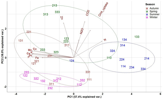
Figure 4.
Distribution of nutrients and GHGs in the two first PCA axes for forest floor data. N: Nitrogen, P: Phosphorus, K; Potassium, Ca: Calcium, Mg: Magnesium, Cu: Copper, Fe: Iron, Mn: Manganese, Zn: Zinc. The 3 digit numbering of the data points represents: the first digit the repetition, the second the treatment (1: Traditional; 2: Selective; 3: Control) and the third digit the season (1: Autumn; 2: Winter; 3: Spring; 4: Summer).
3.6. Relationship of Litterfall Nutrients with Soil GHG Fluxes
Cumulative GHG fluxes were found to correlate significantly with nutrients over four different periods. Taking into consideration the high impact of soil temperature on soil respiration [46], we also categorized our data into two “seasons”, i.e., one “season” including all year except summer, and the summer. In autumn, immediately after thinning, CO2 was found to have a significant positive correlation with Mn (Pearson’s r = 0.76*), whereas the N2O fluxes had a negative correlation to K (r = −0.83 **), Fe (r = −0.67 *) and Zn (r = −0.64 *) (Figure 5a). In winter, CO2 had a significant positive correlation with P (r = 0.69 *) and the N2O fluxes to Ca (r = 0.81 **) (Figure 5b), whereas in spring, only the CO2 fluxes had a significant negative correlation to Cu (r = −0.69 *) (Figure 5e). In summer, the CH4 uptake was recorded as having a significant positive correlation with Ca (r = 0.82 **) (Figure 5f). Except for summer, CO2 showed strong negative correlation with Cu (r = −0.44 *) and Fe (r = −0.41 *), whereas the CH4 uptake was positively correlated with Mg (r = 0.47 *) and N (r = 0.40 *). Regarding the N2O fluxes, there was a strong negative correlation with K (r = −0.56 *), Ca (r = −0.47 *), Cu (r = −0.43 *), Fe (r = −0.58 **) and Zn (r = −0.42 *) (Figure 5c). In total, one year after thinning, the CO2 fluxes were noted having a significant negative correlation with Cu (r = −0.44 **) and Fe (r = −0.43 **), whereas the N2O fluxes had a significantly negative correlation to K (r = −0.46 **), Ca (r = −0.39 *), Cu (r = −0.36 *) and Fe (r = −0.49 **). Non-significant correlations were also detected for the CH4 uptake (Figure 5d and Table 7).
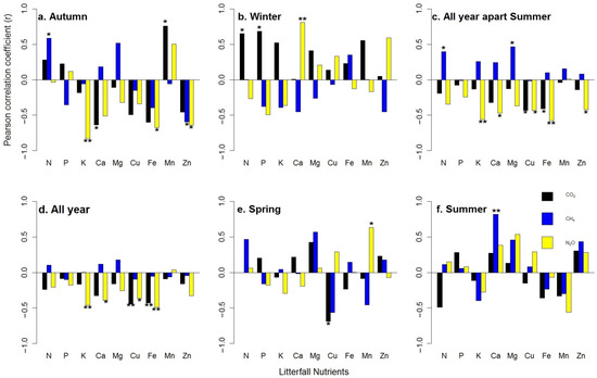
Figure 5.
Seasonal pattern ((a) autumn, (b) winter, (c) all year apart summer, (d) all year, (e) spring, (f) summer) of correlation of litterfall fractions with GHG fluxes over the study period (16 October until 17 September). Asterisks represent significance levels, accordingly: * = 0.05, ** = 0.01. Each bar represents the mean of the three replicates for each treatment (Control, Traditional and Selective).
Table 7.
Pearson correlation analysis among GHG fluxes and litterfall nutrients, one year after thinning, where r: correlation coefficient, p value: significance level.
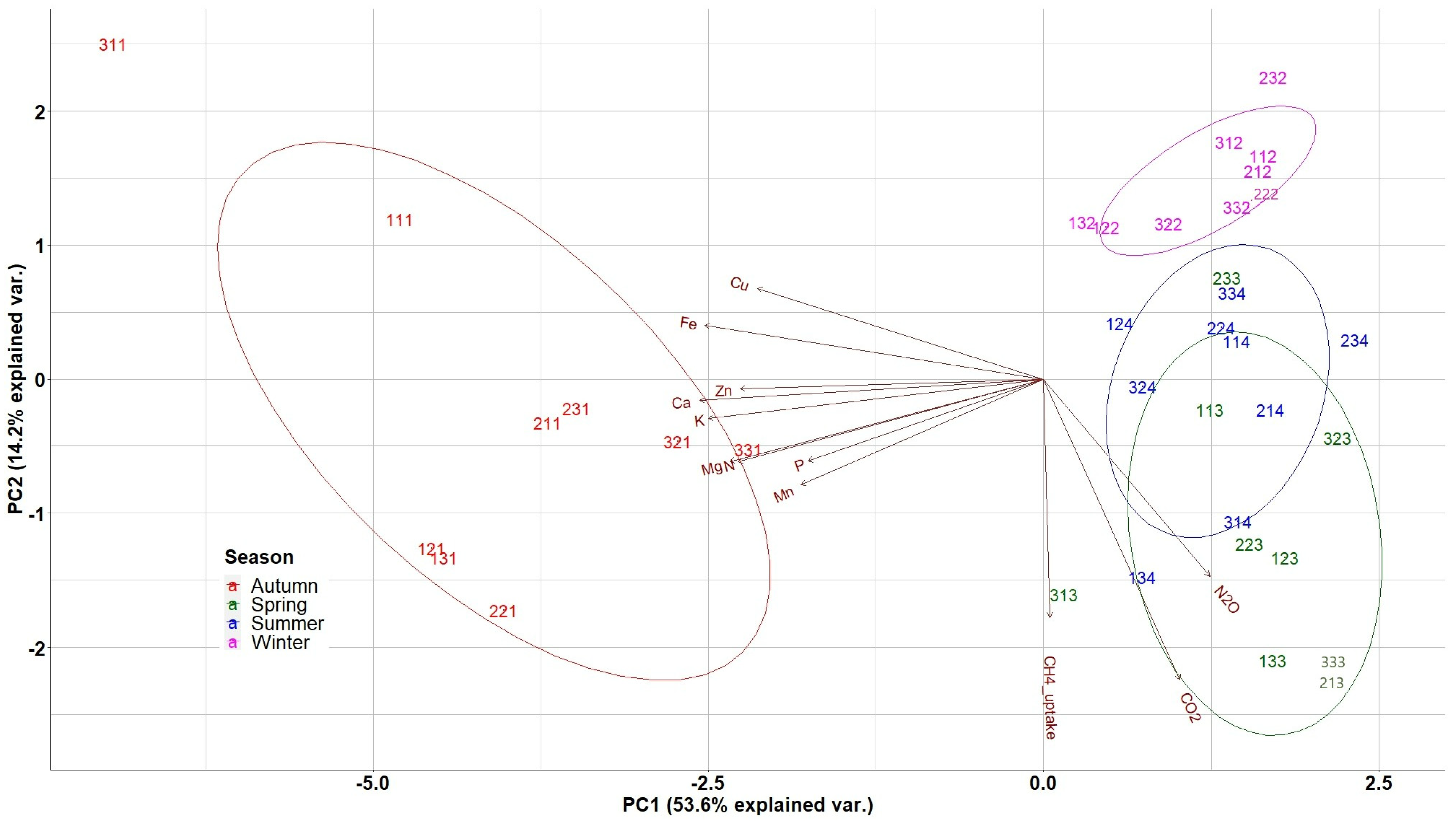
In the biplot of PCA analysis (Figure 6), the weights of the different variables (nutrients, soil GHG fluxes) are presented as arrows and vary by distance from the origin. The biplot enabled the evaluation of the correlation level among the above-mentioned quantified variables, with lines pointing in the same direction being more closely correlated.
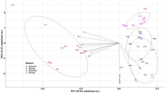
Figure 6.
Distribution of nutrients and GHGs in the two first PCA axes for litterfall data. N: Nitrogen, P: Phosphorus, K; Potassium, Ca: Calcium, Mg: Magnesium, Cu: Copper, Fe: Iron, Mn: Manganese, Zn: Zinc. The 3 digit numbering of the data points represents: the first digit the repetition, the second the treatment (1: Traditional; 2: Selective; 3: Control) and the third digit the season (1: Autumn; 2: Winter; 3: Spring; 4: Summer).
The first group of variables (nutrients), including Cu, Fe, Zn, Ca, K, Mg, N, P and Mn, was very close and highly correlated to the second group, i.e., the group of the soil GHG fluxes including CO2, N2O, and the CH4 uptake. The second group of variables appeared almost perpendicular to the first group and its variables are also close and highly correlated. The first principal component axis (PC1), explaining 53.6% of the variance, was related to the overall seasonal variation of nutrients’ availability in the study site with the negative axis values representing autumn measurements and separating them from summer; thus, the first PCA axis represents the seasonal variation of nutrient availability. The second (PC2) axis, explaining 14.2% of the variance, separated high spring measurements of CO2, N2O and the CH4 uptake (negative axis values) from the respective winter measurements and nutrient concentrations, thus representing the seasonal variation of soil GHG fluxes and litterfall production.
4. Discussion
4.1. Seasonal and Thinning Effects on Nutrients
In our study, the average concentrations of most forest floor nutrients showed a uniform pattern among seasons with highest values in autumn, except for Zn and N, whose highest values were observed in spring and summer, respectively. Similarly, all the litterfall nutrients had higher values in autumn compared to the rest of the seasons. It is also significant that the concentration of most of the litterfall nutrients (N, P, K, Mg, Mn, Z) was higher in spring compared to summer and winter. This is probably caused by the senescence process, reallocating nutrients to other parts of the plant to produce new tissue [11], and takes place in late spring and summer months in a Pinus halepensis forest in Spain.
Our results, in relation to seasonal variation, are similar to those reported in a Nothofagus pumilio forest in Chile, where the highest values of the litterfall nutrients were observed in autumn, followed by summer [23].
Thinning affected forest floor nutrients concentrations. Fe and Zn had the highest concentration in the heavily thinned sites compared to the control. Additionally, thinning affected the nutrient concentration between seasons. In spring, the concentrations of P, N, K, and Mn were affected significantly in both thinned sites, whereas changes in Fe concentration were observed in both spring and summer seasons. On the other hand, no significant changes occurred in the litterfall nutrients due to thinning, although other studies in Pinus halepensis forests showed a reduction of C, K, [11], and Mg [11,47] in needle litterfall in thinned sites compared with controls.
4.2. Thinning Effect on Litterfall Production
In this study, thinning significantly decreased the litterfall production in both treated sites, after just one year of thinning. Litterfall production was decreased by 42.6% in selective thinning plots compared with controls, whereas in traditional thinning the litterfall reduction was found to be less than 1% in comparison with the controls. These results coincide with reports by other studies that showcase thinning’s ability to significantly decrease litterfall production in Spain [20] in Scots pine (Pinus sylvestris) stands, and in Aleppo pine (Pinus halepensis) stands [22]. Çömezet al. [48] stated that thinning practices have different effects on litterfall in Scots pine forests in Turkey, with regard to the age of the stands. Particularly, it was reported that thinning (20–25% removal of the initial basal area) significantly reduced the litterfall production in mature stands, due to the higher stand density in contrast with overmatured stands. This thinning was preferable in mature stands in preventing the excessive reduction of carbon input into the soil through litterfall. Reference [24] reported that thinning significantly changed litterfall production, only for the first year after operation. Additionally, reference [48] claimed that the reduction of litterfall production is attributed to the biomass decrease by thinning rather than altering the litterfall turnover process.
The proportion of pine needle litterfall within total litterfall was higher in summer (65%) and spring (61%), and lower in winter (26%) and autumn (47%). Our results are similar, regarding the highest and the lowest ratio, to those reported by [49] in Calabrian pine (Pinus brutia) forests in South Western Turkey. However, they observed a higher proportion of pine needle litterfall in summer (at 90%), whereas the proportion in winter was slightly higher than our study (at 31%). The low proportion of pine needle litterfall in winter is caused by both high pine bark (38%) and deciduous fractions (mainly reproductive material and deciduous leaves) that was about 21%, and 59% in total. However, it has been reported [49] that the low proportion of pine needle litterfall in winter is due to the high proportion of other conifer fractions (small branches and pine bark that constituted 47%) and not deciduous fractions as at our sites.
Conifer fractions (pine needles and pine bark) were reduced significantly in the heavily thinned plots (selective thinning). These results are partially in agreement with other studies. Several studies [10,22,24] report that more intense thinning affects the pine needle production in litterfall. More specifically, reference [24] reports that, although thinning significantly decreased pine needle and twig production in litterfall, it was not able to affect the total litterfall production or other fractions substantially. Throughout the year of study, the mean pine needle fall production accounted for about 59% of the total litterfall. This percentage is very close to what was reported by [24] (55% for Pinus halepensis). The mean annual cumulative pine needle production was 3.0 Mg·ha−1, which is higher than the 2.30 Mg·ha−1 reported by [24] in a Pinus halepensis plantation, and by [11] in Spain.
The pine needle fall production followed a clear seasonal pattern throughout the study in each of the treatments. The peaks were reported during summer. This matches with other studies that report peak pine needle fall in summer [11,24], while [22] reported a second peak of needle fall in autumn. However, the maximum level of needle fall in summer is common in Mediterranean pine forests due to the dry season with frequent water shortages [20,22]. Similar results were also reported in a Pinus brutia forest in the Antalya Region of Turkey, which boasts a typical Mediterranean climate, where both total litterfall and pine needle litterfall were significantly higher in summer [49].
Pine bark was the second most significant element in the litterfall fraction after pine needles. Thinning has a significant effect on it, which is consistent with other studies in Mediterranean pine forests. It was reported [20] that thinning affected pine bark production considerably in a Pinus sylvestris L. forest located in the Western Pyrenees in Spain. The peak of pine bark fall was also observed in summer. Interestingly, pine bark can easily be detached [50]. We believe that this combination of easy pine bark detachment and the strong winds at the study site over the summer was the primary cause of the high proportion of pine bark fall in summer.
4.3. Relationship between the Litterfall Production and the Soil GHG Fluxes
In the short term (six months after thinning), there were no correlations between the CO2 fluxes and litterfall; on the contrary, the CH4 uptake was strongly correlated to coniferous fractions (pine needles and pine bark). The litterfall layer plays a significant role in soil CH4 exchange with the atmosphere. It is able to control the exchange of CH4 flux with the atmosphere through controlling soil aeration and soil moisture, functioning as a barrier to gas exchange between mineral soil and the atmosphere, consuming either negligible or small amounts of atmospheric CH4 [12,51]. Although there is no direct evidence for coniferous litter, as in the present study, the fresh litter originating from green leaves could produce more CH4 by abiotic factors, such as temperature and solar radiation.
It has been suggested [12] that CO2 fluxes may only be correlated to litterfall layer in providing organic and inorganic compounds present in plant cells for the heterotrophic respiration. Otherwise, CO2 fluxes are not correlated to the litterfall layer. Thus, it is hypothesized in this study that six months after thinning, the oldest of the forest floor substrate had already produced a sufficient level of microbial activity for microbial respiration. This is consistent with [25], which reports that the CO2 fluxes in this period from the study site located in the Monte Morello forest in Italy were strongly correlated with the decomposition of the forest floor. One year after thinning, there was no correlation between the CO2 fluxes and total litterfall production.
Litterfall input is, among other factors, significant in influencing the decomposition rate in forest sites in Greece [52]. Other authors also suggest that the creation of small gaps increased soil organic matter, microbial biomass and C/N ratio, and altered microbiological processes in the upper-soil horizons of Mediterranean conifer forests [25,28,53].
In this study, CH4 uptake was significantly and negatively correlated to conifer fractions and particularly pine needle and pine bark production. Six months after thinning, the CH4 uptake was correlated to the mean C and N stock (3.1 kg·m−2 and 0.14 kg·m−2, respectively) of the forest floor in the deepest soil layers [25]. One year after thinning, the CH4 uptake was significant, but positively correlated to the broadleaved fractions in all the treatments.
Although the total litterfall production decreased throughout the study, deciduous litterfall increased in selective thinning. The increase of broadleaved fractions in a heavily thinned site may have created a barrier for the diffusion of atmospheric CH4 to the soil, and increased the soil’s moisture. This combination is probably what led to an increase of CH4 oxidation and, consequently, CH4 uptake. The creation of small-sized gaps due to thinning, combined with a high content of sand in the soil texture at the study site, can explain not only the increase of the CH4 uptake after thinning [32], but also the significant correlation of deciduous litterfall production with the CH4 uptake.
The N2O fluxes were not correlated with litterfall throughout the year of study. A previous study [25] noted the short-term effects of thinning on GHG emissions and observed that the N2O fluxes were strongly correlated to the N stock in the deepest layer (organic matter, saturated or not) in regard to the forest floor production. In the soil layer close to the surface, no significant correlation was found with N2O fluxes, probably due to the low decomposition rate at this depth that occurs in the Mediterranean conifer ecosystems, where the net mineralization is restricted to the humic layers of the forest floor. This is due to the low level of moisture [25,52]. According to [54], even thoughthinning increases the nitrification, it has no influence on N mineralization. Therefore, it is hypothesized that any alteration of the N2O fluxes resulted probably from the net mineralization at the lower horizon of both the forest floor and litterfall, and that thinning, conversely, had no effect on them.
4.4. Relationship between Nutrients and Soil GHG Fluxes
The forest floor is rich in fungal hyphae, mostly produced by mycorrhizal fungi [55]. Organic phosphorus becomes available through litter decomposition, and the soil pH is reduced, especially when NH4 is present as a result of mycorrhizal activity [13]. The results presented here clearly demonstrate the strong correlation between GHG fluxes and phosphorus (the CO2 fluxes in litterfall and the CH4 uptake in forest floor). Undoubtedly, GHG emissions seem sensitive to soil conditions. Given that mycorrhizal fungi improve the soil structure via hyphae and glomalin production and, in addition, affect the soil environment and microbial activity, it could be argued that they can act as GHG flux regulators.
In this study, a year after thinning, the CH4 uptake was significantly and positively correlated to N and Zn, and negatively to P and Ca nutrients of the forest floor, whereas CO2 was significantly and positively correlated to N and Zn. Such positive correlation of Zn and N to CO2 emissions was reported when these two nutrients were applied as inorganic fertilizer in agricultural fields [56], while no effect on CH4 emissions was described by the same author when Zn chelate fertilizer was used [56].
While this research was able to identify the thinning impacts on litter input nutrients and GHG fluxes, there is one restriction that should be taken into consideration. There was only a short period during which this research was conducted (one year after thinning). Thinning’s impact on soil input nutrients and GHG fluxes may be better understood after three to five years, if the same observations are repeated. A long-term research study of the thinning effect and the formulation of recommendations for selecting parameters (thinning % and predicted impact on soil nutrients input and GHG fluxes) for sustainable forest management methods, will be possible after three or five years.
5. Conclusions
The thinning operations have a significant seasonal effect on both forest floor and litterfall production, and on their nutrient concentration. Despite the short time frame of the study (one year), the results showed that thinning (mainly selective) significantly reduced both total litterfall production and conifer fractions in all thinned sites, with pine needles and pine bark being the most important litterfall fractions. The intense (selective) thinning was also able to numerically increase deciduous litter fractions production, although not to the level of statistical significance, favoring the growth of the understory broadleaved species.
Thinning significantly affected forest floor nutrient accumulation in the intensively thinned sites. Our results suggest that the more that the broadleaved species develop, the greater the soil CH4 uptake. This study contributes to data enrichment, regarding the effect of thinning on litterfall production and nutrient release in the Mediterranean region. However, long-term in situ research is essential in order to evaluate the annual variability of litterfall and the forest floor layers, aiming to extract sound conclusions for management options in global change mitigation targets.
Author Contributions
Conceptualization, F.D.; methodology, F.D., K.R. and A.L.; software, F.D., G.S. and K.K.; data curation, F.D., A.L., M.O., S.S. and E.M.; writing—original draft preparation, F.D.; writing—review and editing, F.D., G.S., M.O., K.R., S.S., K.K., E.M. and A.L.; funding acquisition, K.R. All authors have read and agreed to the published version of the manuscript.
Funding
This research was funded by LIFE project FoResMit “Recovery of degraded coniferous Forests for environmental sustainability, Restoration and climate change Mitigation”, grant number LIFE14 CCM/IT/000905.
Institutional Review Board Statement
Not applicable.
Informed Consent Statement
Not applicable.
Data Availability Statement
The data presented in this study are available on request from the corresponding author. If requested, the corresponding author will ask for data sharing permission from the LIFE programme (LIFE14 CCM/IT/000905).
Conflicts of Interest
The authors declare no conflict of interest.
References
- Ruddell, S.; Sampson, R.; Smith, M.; Giffen, R.; Cathcart, J.; Hagan, J.; Sosland, D.; Godbee, J.; Heissenbuttel, J.; Helms, S.J.L.; et al. The role for sustainably managed forests in climate change mitigation. J. For. 2007, 105, 314–319. [Google Scholar]
- Petsikos, H. Climate change and forest. Part B’. Current issues of applied and forestry policy. In Forest an Integrated Approach; Papageorgiou, A.H., Karetsos, G., Katsadorakis, G., Eds.; WWF Greece: Athens, Greece, 2012; pp. 127–154. [Google Scholar]
- Klein, D.; Höllerl, S.; Blaschke, M.; Schulz, C. The contribution of managed and unmanaged forests to climate change mitigation—A model approach at stand level for the main tree species in Bavaria. Forests 2013, 4, 43–69. [Google Scholar] [CrossRef]
- Warner, D.L.; Villarreal, S.; McWilliams, K.; Inamdar, S.; Vargas, R. Carbon dioxide and methane fluxes from tree stems, coarse woody debris, and soils in an upland temperate forest. Ecosystems 2017, 20, 1205–1216. [Google Scholar] [CrossRef]
- Nave, L.E.; Vance, E.D.; Swanston, C.W.; Curtis, P.S. Harvest impacts on soil carbon storage in temperate forests. For. Ecol. Manag. 2010, 259, 857–866. [Google Scholar] [CrossRef]
- Gelman, V.; Hulkkonen, V.; Kantola, R.; Volusiainen, M.; Volusiainen, V.; Poku-Marboah, M. Impacts of forest management practices on forest carbon. In HENVI Workshop; Helsinki University Centre for Environment: Helsinki, Finland, 2013. [Google Scholar]
- Santilli, M.; Moutinho, P.; Schwartzman, S.; Nepstad, D.; Curran, L.; Volbre, C. Tropical deforestation and the Kyoto Protocol. Clim. Chang. 2005, 71, 267–276. [Google Scholar] [CrossRef]
- Fang, S.; Lin, D.; Tian, Y.; Hong, S. Thinning Intensity Affects Soil-Atmosphere Fluxes of Greenhouse Gases and Soil Nitrogen Mineralization in a Lowland Poplar Plantation. Forests 2016, 7, 141. [Google Scholar] [CrossRef] [Green Version]
- Fahey, T.J.; Woodbury, P.B.; Battles, J.J.; Goodale, C.L.; Hamburg, S.P.; Ollinger, S.V.; Woodall, C.W. Forest carbon storage: Ecology, management, and policy. Front. Ecol. Environ. 2010, 8, 245–252. [Google Scholar] [CrossRef] [Green Version]
- Kunhamu, T.K.; Kumar, B.M.; Viswanath, S. Does thinning affect litterfall, litter decomposition, and associated nutrient release in Acacia mangium stands of Kerala in peninsular India? Can. J. For. Res. 2009, 39, 792–801. [Google Scholar] [CrossRef]
- Bueis, T.; Bravo, F.; Pando, V.; Turrión, M.B. Local basal area affects needle litterfall, nutrient concentration, and nutrient release during decomposition in Pinus halepensis Mill. plantations in Spain. Ann. For. Sci. 2018, 75, 21. [Google Scholar] [CrossRef] [Green Version]
- Peichl, M.; Arain, M.A.; Ullah, S.; Moore, T.R. Carbon dioxide, methane, and nitrous oxide exchanges in an age-sequence of temperate pine forests. Glob. Chang. Biol. 2010, 16, 2198–2212. [Google Scholar] [CrossRef]
- Wang, W.; Peng, C.; Kneeshaw, D.D.; Larocque, G.R.; Lei, X.; Zhu, Q.; Song, X.; Tong, Q. Modeling the effects of varied forest management regimes on carbon dynamics in jack pine stands under climate change. Can. J. For. Res. 2013, 43, 469–479. [Google Scholar] [CrossRef]
- Leitner, S.; Sae-Tun, O.; Kranzinger, L.; Zechmeister-Boltenstern, S.; Zimmermann, M. Contribution of litter layer to soil greenhouse gas emissions in a temperate beech forest. Plant Soil 2016, 403, 455–469. [Google Scholar] [CrossRef] [Green Version]
- Swift, R.S. Macromolecular properties of soil humic substances: Fact, fiction and opinion. Soil Sci. 1999, 164, 790–802. [Google Scholar] [CrossRef]
- Piccolo, A. The supramolecular structure of humic substances: A novel understanding of humus chemistry and implications in soil science. Adv. Agron. 2002, 75, 57–134. [Google Scholar]
- Fuentes, M.; Baigorri, R.; Garcia-Mina, J.M. Maturation in composting process, an incipient humification-like step an multivariate statistical analysis of spectroscopic data shows. Environ. Res. 2020, 189, 109981. [Google Scholar] [CrossRef]
- Hanson, P.J.; Edwards, N.T.; Garten, C.T.; Andrews, J.A. Separating root and soil microbial contributions to soil respiration: A review of methods and observations. Biogeochemistry 2000, 48, 115–146. [Google Scholar] [CrossRef]
- Sulzman, E.W.; Brant, J.B.; Bowden, R.D.; Lajtha, K. Contribution of aboveground litter, belowground litter, and rhizosphere respiration to total soil CO2 efflux in an old growth coniferous forest. Biogeochemistry 2005, 73, 231–256. [Google Scholar] [CrossRef]
- Blanco, J.A.; Imbert, J.B.; Castillo, F.J. Influence of site characteristics and thinning intensity on litterfall production in two Pinus sylvestris L. forests in the western Pyrenees. For. Ecol. Manag. 2006, 237, 342–352. [Google Scholar] [CrossRef]
- Agren, G.I.; Knecht, M. Simulation of soil carbon and nutrient development under Pinus sylvestris and Pinus contorta. For. Ecol. Manag. 2001, 141, 117–129. [Google Scholar] [CrossRef]
- Navarro, F.B.; Romero-Freire, A.; del Castillo, T.; Foronda, A.; Jiménez, M.N.; Ripoll, M.A.; Sánchez-Miranda, A.; Huntsingerd, L.; Fernández-Ondoño, E. Effects of thinning on litterfall were found after years in a Pinus halepensis afforestation area at tree and stand levels. For. Ecol. Manag. 2013, 289, 354–362. [Google Scholar] [CrossRef]
- Caldentey, J.; Ibarra, M.; Hernández, J. Litter fluxes and decomposition in Nothofagus pumilio stands in the region of Magallanes. Chile. For. Ecol. Manag. 2001, 148, 145–157. [Google Scholar] [CrossRef]
- Jiménez, M.N.; Navarro, F.B. Thinning effects on litterfall remaining after 8 years and improved stand resilience in Aleppo pine afforestation (SE Spain). J. Environ. Manag. 2016, 169, 174–183. [Google Scholar] [CrossRef]
- Mazza, G.; Agnelli, A.E.; Cantiani, P.; Chiavetta, U.; Doukalianou, F.; Kitikidou, K.; Milios, E.; Orfanoudakis, M.; Radoglou, K.; Lagomarsino, A. Short-term effects of forest thinning on soil CO2, N2O and CH4 fluxes in Mediterranean peri-urban ecosystems. Sci. Total Environ. 2019, 651, 713–724. [Google Scholar] [CrossRef]
- DeFries, R.; Achard, F.; Brown, S.; Herold, M.; Murdiyarso, D.; Schlamadinger, B.; de Souza, C. Reducing greenhouse gas emissions from deforestation in developing countries: Considerations for monitoring and measuring. Report of the global terrestrial observing system. Land Cover. Glob. Obs. For. Land Cover. Dyn. (GTOS) 2006, 46, 1–20. [Google Scholar]
- Savi, F.; di Bene, C.; Canfora, L.; Mondini, C.; Fares, S. Environmental and biological controls on CH4 exchange over an evergreen Mediterranean forest. Agric. For. Meteorol. 2016, 226, 67–79. [Google Scholar] [CrossRef]
- Butterbach-Bahl, K.; Baggs, E.M.; Dannenmann, M.; Kiese, R.; Zechmeister-Boltenstern, S. Nitrous oxide emissions from soils: How well do we understand the processes and their controls? Philos. Trans. R. Soc. B 2013, 368, 20130122. [Google Scholar] [CrossRef]
- Christopoulou, O.; Polyzos, S.; Minetos, D. Peri-urban and urban forests in Greece: Obstacle or advantage to urban development? Manag. Environ. Qual. Int. J. 2007, 18, 382–395. [Google Scholar] [CrossRef]
- Theodoridis, P. General Introduction. In Management Study of the Public Forestry Division of “Xanthi-Geraka-Kimmerion”. Forest Services Xanthi-Stauroupoli, 2017–2026; Xanthi Forest Directorate: Xanthi, Greece, 2016; Volume 1, pp. 23–34. [Google Scholar]
- IUSS Working Group WRB. World Reference Base for Soil Resources International soil classification system for naming soils and creating legends for soil maps. World Soil Resour. Rep. 2015, 106, 192. [Google Scholar]
- Doukalianou, F.; Radoglou, K.; Agnelli, A.E.; Kitikidou, K.; Milios, E.; Orfanoudakis, M.; Lagomarsino, A. Annual Greenhouse-Gas Emissions from Forest Soil of a Peri-Urban Conifer Forest in Greece under Different Thinning Intensities and Their Climate-Change Mitigation Potential. For. Sci. 2019, 65, 387–400. [Google Scholar] [CrossRef]
- Kitikidou, K.; Milios, E.; Radoglou, K. Single-entry volume table for Pinus brutia in a planted peri-urban forest. Ann. Silvic. Res. 2017, 41, 74–79. [Google Scholar]
- Milios, E.; Kitikidou, K.; Radoglou, K. New Silvicultural Treatments for Conifer Peri-Urban Forests Having Broadleaves in the Understory—The First Application in the Peri-Urban of Xanthi in Northeastern Greece. South-East Eur. For. 2019, 10, 107–116. [Google Scholar] [CrossRef] [Green Version]
- Papaioannou, G. The Torrential Environment of River Kosynthos. Master’s Thesis, Department of Forestry and Management of the Environment and Natural Resources, Democritus University of Thrace, Orestiada, Greece, 2008; p. 118, (In Greek with English Summary). [Google Scholar]
- De Meo, I.; Agnelli, A.E.; Graziani, A.; Kitikidou, K.; Lagomarsino, A.; Milios, E.; Paletto, K.R.A. Deadwood volume assessment in Calabrian pine (Pinus brutia Ten.) peri-urban forests: Comparison between two sampling methods. J. Sustain. For. 2017, 36, 666–686. [Google Scholar] [CrossRef]
- Wright, S.J.; Yavitt, J.B.; Wurzburger, N.; Turner, B.L.; Tanner, E.V.J.; Louis, S.S.; Kaspari, S.M.L.O.; Kyle, H.E.; Hedin, K.E.; Milton, H.N.; et al. Potassium, phosphorus, or nitrogen limit root allocation, tree growth, or litter production in a lowland tropical forest. Ecology 2011, 92, 1616–1625. [Google Scholar] [CrossRef]
- Stevenson, F.J. Nitrogen-organic forms. In Methods of Soil Analysis, Part 2; Page, A.L., Ed.; American Society of Agronomy and Soil Science Society of America: Madison, WI, USA, 1982; pp. 625–641. [Google Scholar]
- Campbell, C.R.; Plank, C.O. Preparation of plant tissue for laboratory analysis. In Hanbook of Reference Methods for Plant Analysis; Kalra, Y.P., Ed.; Soil and Plant Analysis Council Inc.: Boca Raton, FL, USA, 1997; pp. 37–49. [Google Scholar]
- Chadwick, D.R.; Cardenas, L.M.; Misselbrook, T.H.; Smith, K.A.; Rees, R.M.; Watson, C.J.; Williams, K.L.M.J.R.; Cloy, J.M.; Thorman, R.E.; Dhanola, M.S. Optimizing chamber methods for measuring nitrous oxide emissions from plot-based agricultural experiments. Eur. J. Soil Sci. 2014, 65, 295–307. [Google Scholar] [CrossRef]
- Yuesi, W.; Yinghong, W. Quick measurement of CH4, CO2 and N2O emissions from a short-plant ecosystem. Adv. Atmos. Sci. 2003, 20, 842–844. [Google Scholar] [CrossRef]
- IBM Corp. IBM SPSS Statistics for Windows, Version 25.0; IBM Corp.: Armonk, NY, USA, 2017. [Google Scholar]
- R Core Team. R: A Language and Environment for Statistical Computing; R Foundation for Statistical Computing: Vienna, Austria, 2018; Available online: https://www.R-project.org/ (accessed on 10 January 2019).
- Oksanen, J.; Blanchet, F.G.; Friendly, M.; Kindt, R.; Legendre, P.; McGlinn, D.; Minchin, P.R.; O’Hara, R.B.; Simpson, G.L.; Solymos, P.; et al. vegan: Community Ecology Package. R Package Version 2.5–5. 2019. Available online: https://CRAN.R-project.org/package=vegan (accessed on 27 December 2019).
- Vu, V.Q. ggbiplot: A ggplot2 Based Biplot. R Package Version 0.55. 2011. Available online: http://github.com/vqv/ggbiplot (accessed on 10 January 2019).
- Meyer, N.; Welp, G.; Amelung, W. The temperature sensitivity (Q10) of soil respiration: Controlling factors and spatial prediction at regional scale based on environmental soil classes. Glob. Biogeochem. Cycles 2018, 32, 306–323. [Google Scholar] [CrossRef]
- Lado-Monserrat, L.; Lidon, A.; Bautista, I. Litterfall, litter decomposition and associated nutrient fluxes in Pinus halepensis: Influence of tree removal intensity in a Mediterranean forest. Eur. J. For. Res. 2015, 134, 833–844. [Google Scholar] [CrossRef]
- Çömez, A.; Tolunay, D.; Güner, Ş.T. Litterfall and the effects of thinning and seed cutting on carbon input into the soil in Scots pine stands in Turkey. Eur. J. For. Res. 2019, 138, 1–14. [Google Scholar] [CrossRef]
- Erkan, N.; Comez, A.; Aydin, A.C.; Denli, O.; Erkan, S. Litterfall in relation to stand parameters and climatic factors in Pinus brutia forests in Turkey. Scand. J. For. Res. 2017, 33, 338–346. [Google Scholar] [CrossRef]
- Raunemaa, T.; Hart, P.; Kukkonen, J.; Kulmala, M.; Karhula, M. Analysis of the bark of scots pine as a method of studying environmental changes. Water Air Soil Pollut. 1987, 32, 445–453. [Google Scholar] [CrossRef]
- Borken, W.; Beese, F. Methane and nitrous oxide fluxes of soils in pure and mixed stands of European beech and Norway spruce. Eur. J. Soil Sci. 2006, 57, 617–625. [Google Scholar] [CrossRef]
- Kavvadias, V.A.; Alifragis, D.; Tsiontsis, A.; Brofas, G.; Stamatelos, G. Litterfall, litter accumulation and litter decomposition rates in four forest ecosystems in northern Greece. For. Ecol. Manag. 2001, 144, 113–127. [Google Scholar] [CrossRef]
- Muscolo, A.; Settineri, G.; Bagnato, S.; Mercurio, R.; Sidari, M. Use of canopy gap openings to restore coniferous stands in Mediterranean environment. iForest-Biogeosci. For. 2017, 10, 322. [Google Scholar] [CrossRef] [Green Version]
- Hart, S.C. Potential impacts of climate change on nitrogen transformations and greenhouse gas fluxes in forests: A soil transfer study. Glob. Chang. Biol. 2006, 12, 1032–1046. [Google Scholar] [CrossRef]
- Smith, E.S.; Read, D. Mycorrizas in ecological interactions. In Mycorrhizal Symbiosis, 3rd ed.; Academic Press: Cambridge, MA, USA, 2008; p. 573. ISBN 978-0-12-370526-6. [Google Scholar]
- Montoya, M.; Castellano-Hinojosa, A.; Vallejo, A.; Álvarez, J.M.; Bedmar, E.J.; Recio, J.; Guardia, G. Zinc fertilizers influence greenhouse gas emissions and nitrifying and denitrifying communities in a non-irrigated arable cropland. Geoderma 2018, 325, 208–217. [Google Scholar] [CrossRef]


Publisher’s Note: MDPI stays neutral with regard to jurisdictional claims in published maps and institutional affiliations. |
© 2022 by the authors. Licensee MDPI, Basel, Switzerland. This article is an open access article distributed under the terms and conditions of the Creative Commons Attribution (CC BY) license (https://creativecommons.org/licenses/by/4.0/).