Modelling the Impact of National vs. Local Emission Reduction on PM_2.5 in the West Midlands, UK Using WRF-CMAQ

Abstract

Ambient air pollution from PM_2.5 is a major risk to human and environmental health, with significant impacts on mortality and morbidity. Mitigation policies—which may be regional or national in extent—need to consider both primary and secondary particles to be effective, balancing within-region emissions and longer-range transport phenomena. The modelling system WRF-CMAQ was used to simulate the impact of emissions reductions in the West Midlands region of the UK, evaluating the change in total PM_2.5 and in its primary and secondary components. Domestic combustion, road transport and agriculture emissions were reduced individually or in combination, at a national or at local level. Combined reduction of road transport and agriculture emissions showed the strongest reduction (29%) in average PM_2.5 if applied at national level. At the local level, reductions from domestic combustion were shown to be the most effective policy (13.4% on average). Secondary inorganic fractions of PM_2.5 are the most abundant, with 25% NO₃⁻ 21% SO₄²⁻ and 13% NH₄⁺ on average. Scenario analysis shows that the contribution of secondary components to the fractional change of PM_2.5 dominates for national policies (up to 0.86 for NO₃⁻) when road transport and agriculture activities are reduced, while at the regional level the elemental and organic carbon fractional changes are dominant (up to 0.64 for organic carbon).

1. Introduction

Several steps have been taken in the last decade to improve air quality in the United Kingdom. Mitigation policies at a national level, alongside technological and societal changes, have led to significant reductions in PM_2.5 concentrations, by 23 and 26% at urban and roadside locations, respectively [1]. Despite this, the recent changes made by the World Health Organisation (WHO) to guideline levels for the protection of human health, lowered to 5 µg/m³ for annual mean PM_2.5 concentrations, call for further efforts aimed at reducing anthropogenic emissions, especially where these impact urban areas [2].

The West Midlands (WM) is the second-most populous region of the UK after Greater London, with more than 2.9 million inhabitants. It includes the UK’s second-largest city, Birmingham, with 1.1 million inhabitants. UK government projections predict the WM to have one of the highest population growth rates (+7.5%) in the period 2015–2025 [3]. This rapid population growth and urbanisation will potentially increase total population exposure to air pollution in the region.

Within the UK, the National Atmospheric Emissions Inventory (NAEI, [4]) indicates that 38% of primary PM_2.5 emissions in the UK are generated by domestic combustion, including biomass, wood and coal burning in closed stoves and open fires [5]. Road transport also makes a significant contribution to primary PM_2.5 (12%), despite an 85% decrease in exhaust emissions since 1996 due to stricter emission standards [6]. Another pollutant contributing to secondary formation of PM_2.5 is ammonia (NH₃). During the short time this gas persists in the atmosphere (e.g., a few hours) it reacts with other gases such as nitrogen oxides and sulphur dioxide to form secondary PM species such as ammonium nitrate and ammonium sulphate, which remain suspended for a few days in the atmosphere and are often transported over large distances [7]. In total, 88% of UK ammonia is emitted by agricultural activities, with minor contributions from waste (2.5%) and transport (1.7%).

Additionally, approximately 30% of the total PM_2.5 mass concentration in the UK comprises secondary inorganic aerosols (SIA); this percentage reaches 44% of the total concentration in the city of Birmingham [8]. Studies in the WM have shown that NO₃⁻, SO₄²⁻ and NH₄⁺ secondary inorganic fractions were the main constituents of PM_2.5 in WM urban areas, followed by carbonaceous fractions of organic and elemental carbon (OC and EC) [9]. To maximise the effects of national and local environmental policies, it is important to analyse the influence that potential emissions reductions have not only on total PM_2.5 but also on its individual components. Health impacts are likely to be affected by PM mass concentration (PM_2.5), composition, particle size and morphology—including ultrafine particle number concentrations—however, our focus here is PM_2.5 mass concentration and bulk composition.

Chemistry-transport models (CTMs) have frequently been used to simulate aerosol formation, composition, dispersion, and transport. Within the UK/European context, some recent studies have focused on the effect of long-range transport of aerosols from north-west Europe to the UK [10,11] while others focused on the sensitivity of final concentrations to primary PM_2.5 emission reductions for present and future periods [12]. The impact of policy options and in particular of anthropogenic emission reduction has been investigated using different types of models and CTMs (e.g., among the most recent [13,14,15]). Finally, while some works have focused on high-resolution numerical simulations over the city of London [16,17], none have previously addressed the impact of national vs. regional primary PM_2.5 emission reductions on total and individual secondary inorganic fractions in the West Midlands.

In this work we use the modelling system WRF-CMAQ to simulate average concentrations of PM_2.5 and the main fractions of NO₃⁻, SO₄²⁻, NH₄⁺, EC and OC for January and July 2016, representing winter and summer conditions. We simulate PM_2.5 changes for scenarios with reduced anthropogenic emissions from road transport, agriculture, and domestic combustion activities, applying a reduction to (i) the emissions from these sectors across the whole UK, and (ii) emissions limited to the WM area. Finally, we evaluate the changes in monthly average concentrations of PM_2.5 and its main individual chemical components.

The paper is organised as follows: Section 2 describes the main characteristics of the modelling system and the configuration used for the simulations. Section 3 shows the results of evaluation of the modelling system in comparison with observations, using different metrics, the results of scenarios with reduced anthropogenic emissions and the fractional concentration change of PM_2.5 components. Finally, Section 4 summarises the conclusions and proposed future developments.

2. Materials and Methods

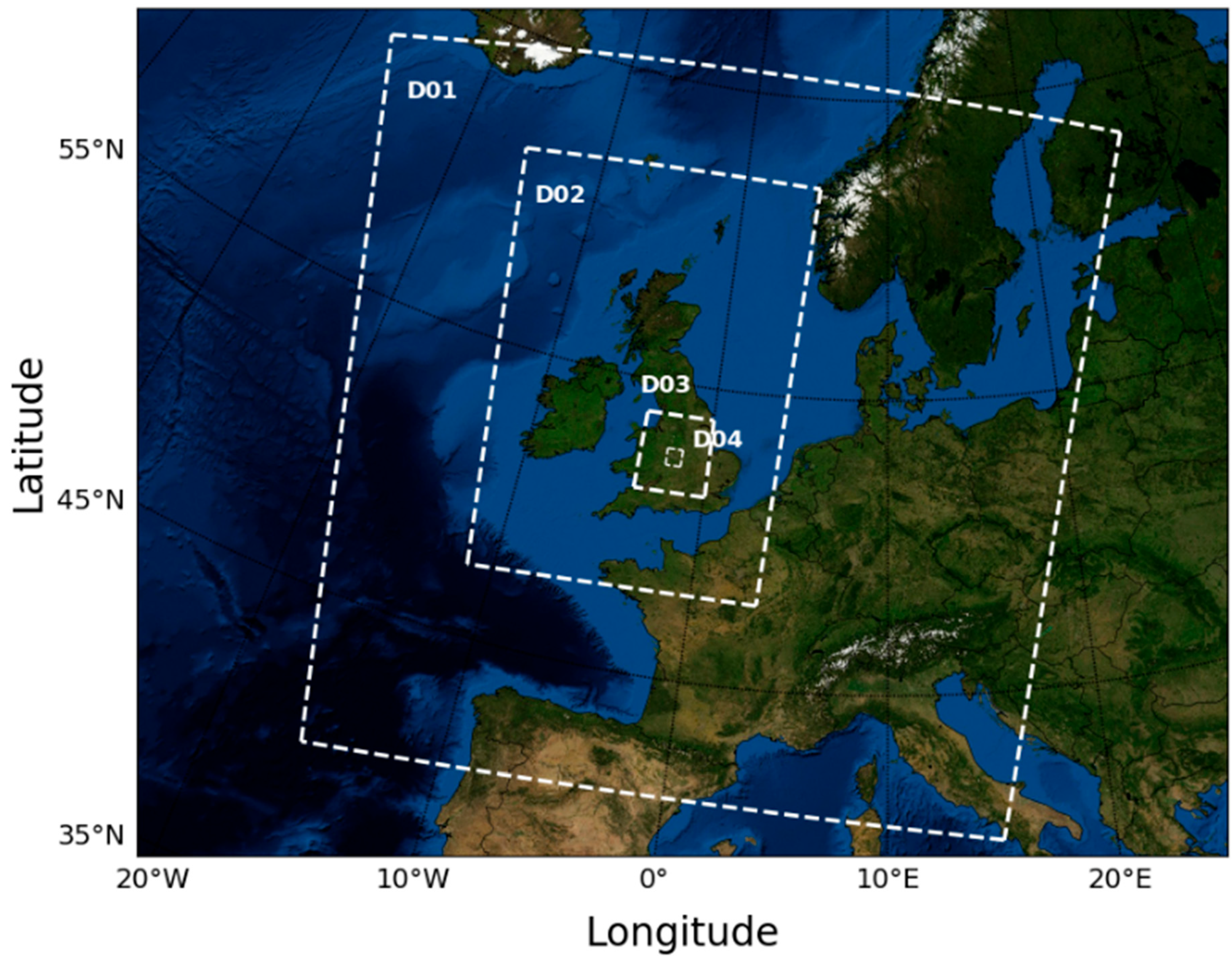
2.1. Modelling System

Meteorology and chemistry transport processes over the West Midlands have been simulated using the Weather Research and Forecasting (WRF) model, version 3.9.1 [18] and the Community Multi-Scale Air Quality Model (CMAQ), version 5.2.1 [19]. WRF is a next-generation mesoscale numerical model developed to perform operational forecasts and atmospheric research through weather simulations. WRF incorporates multiple options for different physical parametrisations for the simulation of tropospheric weather fields. CMAQ is an open-source numerical model developed by the USEPA for the simulation of chemistry and transport processes in the low troposphere involving a large range of air pollutants. CMAQ is widely used for research and regulatory purposes by academics and policy makers for the simulation of air pollution levels, creations of forecasts, and scenarios with reduced emissions for policy making.

Both models have been configured to run simulations on 4 nested domains at increasing spatial resolutions. A coarse domain at 27 × 27 km covers most of western continental Europe, two intermediate domains at 9 × 9 km and 3 × 3 km are centred on the UK and Southern England, while the finest domain at 1 × 1 km is centred on the West Midlands area. (Figure 1). The WRF-CMAQ grid includes 30 vertical levels with the first at 20 m from the ground and 9 in total below 1 km height.

The adopted WRF configuration follows the parameters recommended by the “CMAQ Development for UK National Modelling Report” (CMAQ4UK) [20,21]. Initial and boundary conditions are derived from the European Centre for Medium-Range Weather Forecast (ECMWF) ERA 5 reanalysis [22]. These IC/BC are created using forecasts at 31 km resolution (one-fourth the spatial resolution of the operational model). They integrate 137 hybrid sigma-pressure levels in the vertical, up to 0.01 hPa. The choice of the ECMWF IC/BC is motivated by the evidence shown in previous works focused on the optimisation of the WRF configuration for the UK, relating to the influence that initial and boundary conditions used in WRF have on both meteorological patterns and on conditions of regional air quality [23]. Grid nudging has been applied every 6 h to constrain WRF outputs to observations, with nudging coefficients defined for U and V wind components, temperature (T) and water-vapour-mixing ratio (Q). The process permits to constrain the values of selected variables (e.g., U, V, T and Q) calculated by WRF to the original re-analysis value from the data used by WRF (e.g., ECMWF) with a certain frequency of time (e.g., 6 h).

The CMAQ configuration uses initial and boundary conditions for the outermost domain created using seasonal average hemispheric CMAQ outputs for the year 2016, distributed through the CMAS data warehouse. These data were generated using CMAQv5.3 with spatial resolution of 108 × 108 km on a polar stereographic grid covering the northern hemisphere. Species concentrations have been mapped to the CB05 mechanism using the ‘combine’ program from the CMAQ post-processing toolkit before being used to create the initial and boundary conditions for the domain at 27 km resolution. The internal domains at 9 km, 3 km, and 1 km resolution draw initial and boundary conditions from the respective parent domain. These IC/BC have been created using the ICON and BCON modules internal to CMAQ. The Carbon Bond 05 (CB05) chemical mechanism has been adopted for all simulations. It was developed in 2005 and is a condensed mechanism of atmospheric oxidant chemistry for 51 species and 156 reactions, suitable for modelling ozone, particulate matter, visibility, acid deposition and air toxics issues [24]. A summary of the main settings of the WRF-CMAQ configuration is given in Table 1.

The UK NAEI [4] has been merged with the regional emission inventory CAMSv3.1 [25] to provide a comprehensive description of anthropogenic emissions for the UK and northwest Europe. Both emission inventories provide annual totals of anthropogenic sources for the year 2016 and have been disaggregated spatially and temporally over the simulation domains using appropriate pre-processing tools: EMIT [26] for NAEI and HERMES [27] for CAMSv3.1, then merged by pollutant on each grid. EMIT and HERMES were used to disaggregate the emission rates from the original emission inventories (in annual totals) on spatial grids at different resolution (from 27 × 27 km to 1 × 1 km). Moreover, the tools also provide temporal and vertical profiles of the emissions from annual totals to hourly fluxes according to emission coefficients diversified by pollutant and by sector. These profiles for the disaggregation of both emission inventories have been taken from EMEP model inputs [28]. Finally, biogenic emissions used in this work come from MEGAN software, version 3.1 [29]. The leaf area index data for 2016 has been taken from the European Union’s Earth observation programme Copernicus [30] and implemented in MEGAN for the calculation of biogenic emissions.

Table 1. WRF and CMAQ configuration used for simulations and scenarios.

WRF Configuration		CMAQ Configuration
WRF version	3.9.1	CMAQ version	5.2.1
IC/BC	ECMWF ERA5	Sp. Projection	Lambert Conformal Conic
Land use	USGS	IC/BC	CMAQ Hemispheric Outputs
Urban Physics	BEP	Chemical Scheme	CB05e51_ae6_aq
Boundary Layer	BouLac	Anth. Emissions	CAMS3.1/NAEI
Surface Layer	Monin	Temp. Profiles	Simpson et al., 2012 [28]
Land surface	NOAH	Natural Emis.	MEGAN3.1
Vertical Levels	30	Vertical Levels	30

Table 1. WRF and CMAQ configuration used for simulations and scenarios.

WRF Configuration		CMAQ Configuration
WRF version	3.9.1	CMAQ version	5.2.1
IC/BC	ECMWF ERA5	Sp. Projection	Lambert Conformal Conic
Land use	USGS	IC/BC	CMAQ Hemispheric Outputs
Urban Physics	BEP	Chemical Scheme	CB05e51_ae6_aq
Boundary Layer	BouLac	Anth. Emissions	CAMS3.1/NAEI
Surface Layer	Monin	Temp. Profiles	Simpson et al., 2012 [28]
Land surface	NOAH	Natural Emis.	MEGAN3.1
Vertical Levels	30	Vertical Levels	30

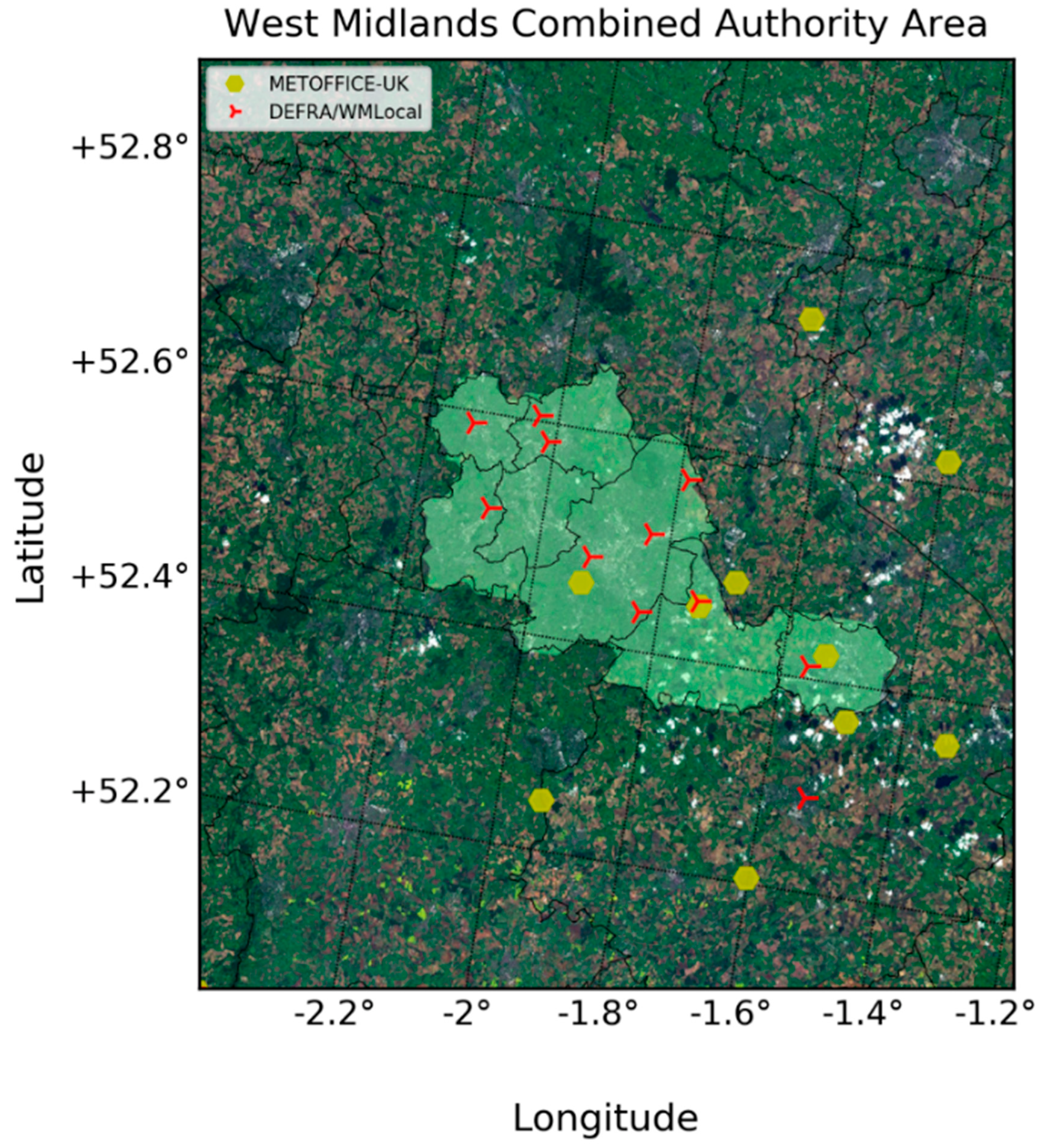
2.2. Simulation Period and Observation Sites

The simulations using WRF and CMAQ were conducted for two monthly periods representative of winter and summer conditions of 2016, namely January and July, applying a spin-up period of 5 days before the formal start of the simulations of both models.

The simulation months were chosen as those showing the highest mean temperature during summer and lowest during winter (around 17 and 5 °C, respectively for the domain in Figure 2) in comparison to the average annual value of 10 °C. Moreover, during these two months no extreme weather events (e.g., rainstorms, heat waves) impacting the common weather condition were recorded. The simulation year of 2016 was defined to make use of the most up-to-date nationally ratified anthropogenic emissions for the UK available at the time of model development.

Ten meteorological measurement stations in the WM have been used for the validation of WRF (Figure 2). Surface temperature, wind speed and direction data used for the validation come from the Met Office UK database for 2016 [31], while relative humidity was calculated using the coefficients proposed by Alduchov and Eskridge [32] based on hourly observed values of surface and dew point temperatures. U and V vector components of wind speed were calculated by combining observed values of wind speed and direction. A total of 11 stations were used for the validation of PM_2.5 in CMAQ. All stations are representative of urban background: 7 from the West Midlands local authority network and 4 from the AURN-DEFRA national network (Figure 2).

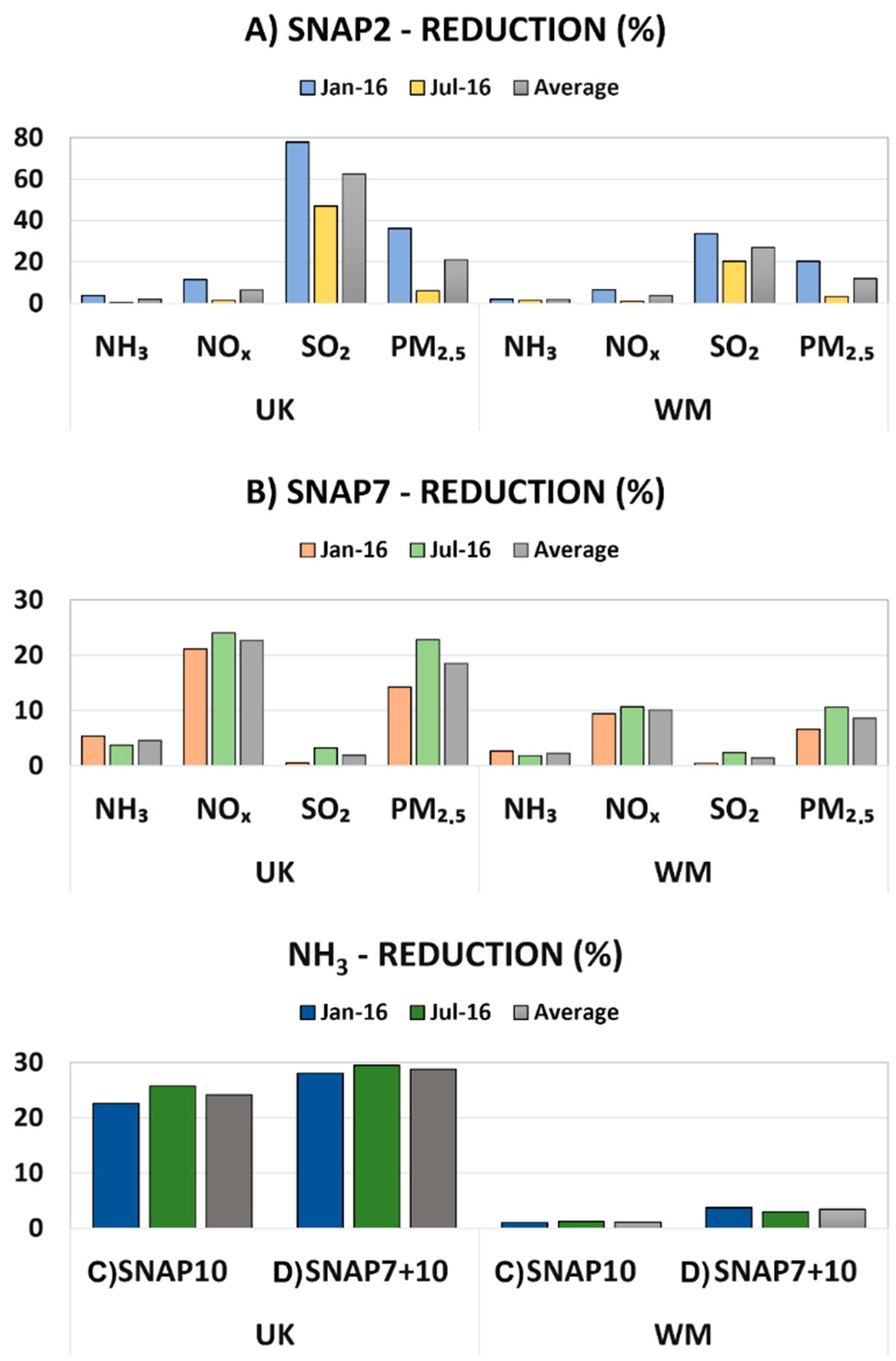
2.3. Scenario Design

According to the UK Clean Air Strategy 2019 [5], 38% of primary PM_2.5 emissions are generated by domestic wood and coal burning, followed by industrial combustion (16%) and road transport (12%), among others. Besides this, secondary PM is formed in the atmosphere through chemical reactions between gaseous pollutants such as NO_X, SO₂ and NH₃ generated by road transport, industrial and agricultural activities, and following the chemical processing and condensation of organic components.

Three scenarios have been created considering the following emissions changes: 85% reduction of all emissions from the SNAP2 sector (A), corresponding approximately to removal of domestic combustion activities related to coal, coke and wood burning; 30% reduction of ammonia emissions (only) from the SNAP10 (agriculture) sector (B); and 30% reduction of (all) road transport emissions (SNAP7, C). A fourth scenario combining the reductions in SNAP7 and SNAP10 (D) was created to consider the combined effect of possible mitigation policies (

Table 2. Percentage of reduction of sector emissions calculated for each scenario simulated in CMAQ.

Label	Sector	Description	Reduction
A	SNAP2	Domestic Combustion	85%
B	SNAP7	Road Transport	30%
C	SNAP10	NH3 agriculture	30%
D	SNAP7+10	Road transport + NH3 agriculture	30 + 30%

). Scenarios A and C were designed by reducing primary emissions of all pollutants included in the respective sectors, while in scenario B, emissions from NH₃ alone were reduced.

Scenario A was designed to explore a near-total removal of solid fuels from domestic combustion activities. Wood, coal and coke burning represent the highest source of emissions connected to domestic combustion in the NAEI and can impact both primary and secondary formation of PM_2.5. According to the NAEI, wood burning generates approximately 85% of primary emissions of PM_2.5 from the whole sector, hence this magnitude of emissions reduction was selected. Coal and coke burning are responsible for 22 and 56% of SO₂ and 3 and 2% of NO_X emissions (respectively) from SNAP2 [4] and so represent probable further contributors to PM secondary formation in the atmosphere. Approximately 30% of wood fuel used in UK is sourced from the informal “grey” wood market, and 90% of domestic wood users use logs either solely or in conjunction with other fuels (pellets, briquettes, waste wood, gathered wood, and wood chips) [33]. Due to these complications, the reduction of emissions of individual pollutants by fuel type (e.g., wood vs. coal) is difficult to estimate and therefore reduction in all primary emissions from the SNAP2 sector was chosen.

Scenario B for road transport emissions represents reduction of all emissions across the vehicle fleet, including emissions from exhaust, brakes and tyres, and different fuel types. In this respect, it does not reflect the expected transition to electric vehicles, for which most non-exhaust particulate emissions would remain. The reduction of 30% was selected to align with the anticipated impact of the UK Clean Air strategy to meet National Emission Ceiling Regulation limits in 2030 for the road-transport sector [34]. Similar to scenario A, the reduction in primary emissions (30%) was applied to each pollutant present in the sector. Finally, scenario C was designed to reflect changes in agricultural practices reducing emissions of NH₃ only, while keeping all other sector pollutant emissions unchanged. Ammonia emissions from this sector arise from plant production, fertilisation, and livestock manure and the reduction is an important component of the UK Net Zero Strategy [35]. Similarly to scenario B, the reduction of 30% ammonia emissions in scenario C was set considering the ammonia emission reduction ceiling planned for the year 2030 and included in the Clean Air Strategy [5].

The four scenarios have been applied to represent policy applications on either a local/regional or a national basis. The emissions have been manipulated in two different ways: (1) a comprehensive reduction of UK emissions in all domains (hereafter called UK case), simulating national policy effects. Emissions from CAMSv3.1 inventory for northwest Europe included in the 27 and 9 km domains were unchanged (no reduction). (2) A reduction of emissions only within the masked area of the West Midlands, (hereafter called WM case), simulating the effects of potential regional (only) policies (Figure 2).

Percentage reductions of total NH₃, NO_X, SO₂ and primary PM_2.5 emissions are shown for scenarios A and B, while for scenarios C and D we show only the reduction in NH₃ (Figure 3). The domestic combustion emission reduction (A) has the strongest effects on SO₂ and PM_2.5 emissions both in winter and summer, with average emission reductions of 62 and 21% for the UK case and 27 and 16% for the WM case, respectively. The reduction in road transport emissions (B) affects both NO_X and primary PM_2.5, with average emission reductions of 23 and 18% for the UK case and 10 and 8% for the WM case, respectively.

Finally, the proportional reductions of NH₃ emissions in scenarios C and D for different domains are substantially different: 24 and 29% for the UK case and 1 and 3% for the WM case, respectively. This difference in emission reduction is connected to the limited extent of agricultural activity inside the WM borders. The majority of these (agricultural) emissions are, in fact, included in the 1 × 1 km domain but outside the WM masked area and therefore altered only in the UK scenarios.

The effect of the emissions reductions from the four scenarios on PM_2.5 concentrations have been analysed in term of the most abundant components: NO₃⁻, SO₄²⁻, NH₄⁺, EC and OC for both UK and WM cases using the fractional change in concentrations (FC) (Equation (1)):

$$FC=\frac{1}{N}{\displaystyle \sum }_{i=1}^N\frac{B_i-C_i}{B_i}$$

(1)

where $N$ is the total number of ground level computational cells within the domain, $B_i$ is the base case predicted value of the pollutant concentration in cell $i$ and C_i is the predicted value of the pollutant concentration in cell $i$ for the relevant scenario.

3. Results

3.1. Modelling System Validation

The validation of the combined WRF-CMAQ modelling system has been carried out for the domains at 9, 3 and 1 km resolution. In this work we present the results of the validation of the finest resolution domain at 1 × 1 km for both models, limited to surface data due to the absence of sites providing vertical sounding inside the domain area.

Mean normalised bias (MNB), root mean square difference (RMSD), index of agreement (IOA) and Pearson’s coefficient (R) have been used to quantify the performance of the models against observations (

Table 3. Statistical operations used for the validation of the modelling system WRF-CMAQ for the simulation periods. M_i is the modelled value at the time i, O_i is the observed value at the time i.

Operation	Formula
Mean Normalised Bias (MNB)	$\frac{{{\displaystyle \sum }}_{i=1}^n\left(M_{i }-O_i\right)}{{{\displaystyle \sum }}_{i=1}^n(O_i)}$
Root Mean Square Difference (RMSD)	$\sqrt{\frac{{{\displaystyle \sum }}_{i=1}^n{\left(M_i-O_i\right)}^2}{n}}$
Index of Agreement (IOA)	$1-\left[\frac{{{\displaystyle \sum }}_{i=1}^n{\left(O-M\right)}^2}{{{\displaystyle \sum }}_{i=1}^n{\left(\left|M-\overline{O}\right|+\left|O-\overline{O}\right|\right)}^2}\right]$
Pearson’s Coefficient (R)	$\frac{n\left({{\displaystyle \sum }}_{i=1}^n{M}_i{O}_i\right)-\left({{\displaystyle \sum }}_{i=1}^n{M}_i\right)\left({{\displaystyle \sum }}_{i=1}^n{O}_i\right)}{\sqrt{\left[n{{\displaystyle \sum }}_{i=1}^n{M}_i^2-{\left({{\displaystyle \sum }}_{i=1}^n{M}_i\right)}^2\right]\left[n{{\displaystyle \sum }}_{i=1}^n{O}_i^2-{\left({{\displaystyle \sum }}_{i=1}^n{O}_i\right)}^2\right]}}$

).

The performance of WRF in simulating temperature and relative humidity shows a correlation (R) between 0.95 and 0.90 for the former and 0.57 and 0.69 for the latter. While the surface temperature tends to be underestimated in winter (−0.13) and in summer (−0.15) from the mean normalised bias (MNB), the opposite is found for the relative humidity (0.06 in winter and 0.18 in summer). The index of agreement (IOA) for these two variables is higher for the temperature (93% in winter and 90% in summer) than for relative humidity (52% in winter and 69% in summer) (

Table 4. Statistical evaluation of WRF calculated for 2016 for surface parameters of Temperature (°C), relative humidity (%), wind speed (ms⁻¹) and direction (degrees) and U and V components of wind (ms⁻¹).

Jan-16	V	U	W Sp.	W Dir.	Temp.	RH
Mean Obs	2.04	0.82	3.74	197.43	5.27	89.54
Mean Model	1.93	1.01	4.47	197.06	4.59	94.98
MNB	−0.05	0.23	0.19	0.003	−0.13	0.06
RMSD	2.33	1.88	2.14	66.7	1.50	8.78
IOA	0.70	0.80	0.55	0.60	0.93	0.52
R	0.80	0.88	0.72	0.77	0.95	0.57
Jul-16	V	U	W Sp.	W Dir.	Temp.	RH
Mean Obs	0.96	1.99	2.96	240.69	16.99	76.64
Mean Model	1.23	2.24	3.34	241.74	14.33	90.60
MNB	0.28	0.12	0.13	0.005	−0.15	0.18
RMSD	1.50	1.45	1.64	55.1	3.27	17.7
IOA	0.76	0.66	0.52	0.51	0.90	0.69
R	0.87	0.81	0.71	0.72	0.82	0.60

).

WRF is able to reproduce the main wind speed and direction with correlation (R) between 0.71 and 0.72 for wind speed and between 0.72 and 0.77 for wind direction that tends to be better reproduced in January than in July. The MNB is found to lie between 0.13 and 0.19 and between 0.003 and 0.005 for wind speed and direction, respectively. Finally, the IOA for both variables is between 52 and 55% (wind speed) and 51 and 60% (wind direction) suggesting that the model better reproduces the wind components during the summer period.

The statistics for wind speed and direction are confirmed in the decomposition of the winds into U and V vector components. The correlation (R) is found between 0.80 and 0.88 in January and 0.81 and 0.87 in July. The MNB is found positive in July for both U and V (0.12 and 0.28, respectively) while in January it is positive for U (0.23) and negative for V (−0.05). The IOA is between 70 and 76% for V and between 66 and 88% for U between the two periods.

The statistical evaluation of CMAQ in reproducing PM_2.5 concentrations in January and July 2016 is shown in

Table 5. Statistical evaluation of CMAQ calculated for January and July 2016 for PM_2.5 from urban background stations in the 1 × 1 km domain shown in Figure 1.

PM2.5	Jan-16	Jul-16
Mean Obs	7.95	6.23
Mean Model	4.93	3.60
MNB	−0.38	−0.42
RMSD	2.19	1.55
IOA	0.72	0.57
R	0.67	0.41

. The model tends to underestimate the average concentration during winter (−0.38) and summer (−0.42), according to the MNB values. Despite this higher correlation (R) and index of agreement values are found during January (0.67, 72%) than July (0.41, 57%). The reason for this difference can be attributed to the higher photochemistry acting in the atmosphere in July that could have an influence on the secondary formation of aerosol components not well captured by the model (Table 5).

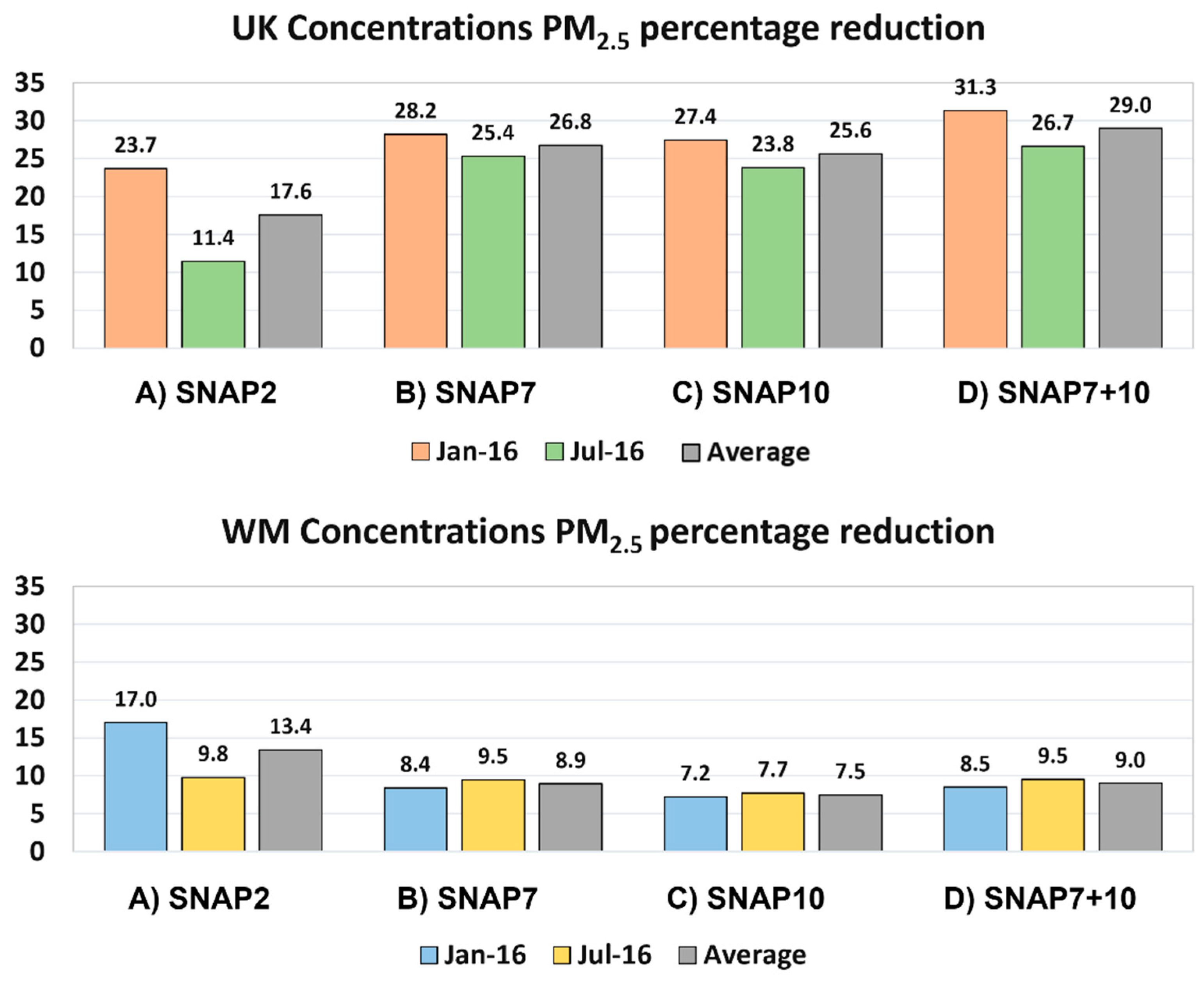
3.2. PM_2.5 Changes for Each Scenario

The effects of the emission reduction scenarios on concentrations of PM_2.5 have been tested. The percentage reductions of concentrations have been calculated for the WM area as shown in Figure 1, excluding all the cells outside the region.

Scenarios simulating possible national mitigation policies (UK case) show that of the scenarios considered, the combined reduction of road transport and agriculture sectors provide the largest decrease of PM_2.5 in both simulated periods (Figure 4, top). Scenarios representing mitigation policies applied at the local level only (WM case) show that the scenario with strongest effect on the final PM_2.5 concentrations within the region was the SNAP2 reduction (Figure 4, bottom). Comparing the difference in PM_2.5 reduction from the UK to the WM case, we find that scenario A leads to, on average, 4.2% difference between national and regional-only emissions changes, while scenarios B and C show a higher difference between these two approaches of around 18%. Finally, scenario D shows the greatest difference between the UK and WM-only cases, of around 20%.

The difference in PM_2.5 concentration reductions between the UK and WM cases for scenarios B, C and D highlights that agriculture and road transport emissions outside the WM area make a substantial contribution to the final concentrations of PM_2.5 within the region. For scenario B, this is linked to the main road arteries connecting the West Midlands with the north, east (the M6) and south part of the country (the M40 and M5) extending outside the WM mask and not considered in the WM reduction cases. For scenario C, ammonia emissions are located almost completely outside the WM borders, due to the largely urban character of the WM region. The impact of ammonia reduction on PM_2.5 was already highlighted by Vieno et al., 2016 [12] as one of the most influential sources in agricultural and natural areas. Hence the reduction of agricultural ammonia alone, or in combination with road transport reductions, would be more effective as a national policy (UK case). In contrast, the domestic combustion scenario (A), despite being a source with high seasonal variability, shows the largest reduction in PM_2.5 in response to WM region-only mitigation policies (13.4% on average, with substantially larger benefits in winter, when PM_2.5 concentrations are greatest), of the scenarios considered. The reduction in PM_2.5 achieved for region-only domestic combustion emission reductions is similar to that found for equivalent national policies (17.6%) suggesting that the main influence comes from sources located inside the WM region, which can effectively be addressed by local and regional mitigation policies.

The effects of reductions in primary NO_X, SO₂ and NH₃ emissions on concentrations of PM_2.5 in the UK context have previously been highlighted by the Air Quality Expert Group (AQEG, [36]). The greatest impact upon PM for reduction of a single species’ emissions corresponded to reduction in primary ammonia, which was followed by the reduction in SO₂ and substantially higher than the reduction in NO_X only. Results obtained by AQEG showed also that lowest concentrations of PM_2.5 comes from the combined reduction of primary PM_2.5 and NH₃. This result is in line with the UK scenario with agriculture (NH₃ only from B) and road transport activities (all primary emissions including PM_2.5 from C) simultaneously reduced by 30%.

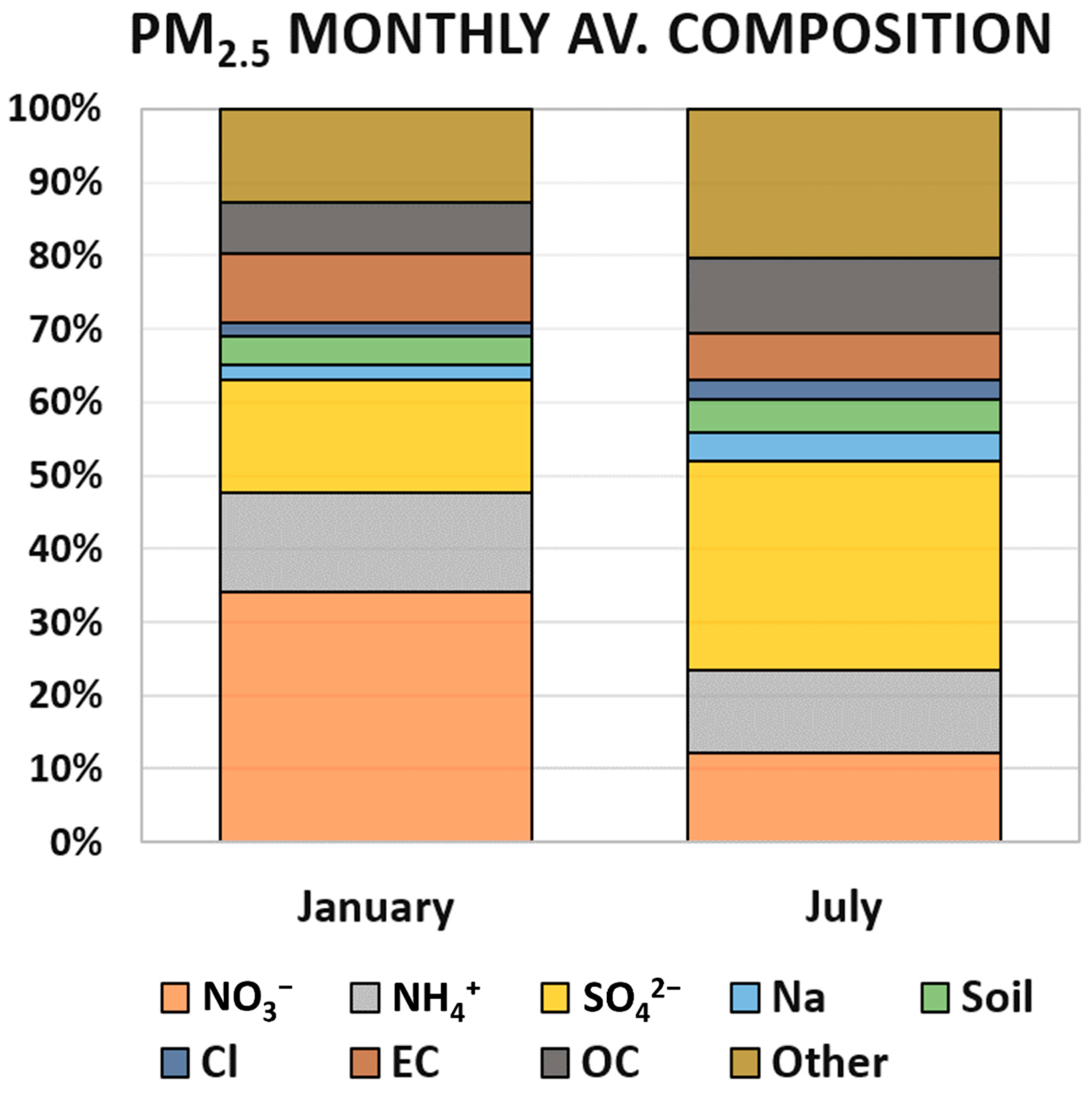
3.3. Scenario Effects on PM_2.5 Components

Model outputs for the reduced emissions scenarios have been analysed to assess the change in individual components of PM_2.5, calculated from the base case simulations inside the WM masked area (Figure 5). Results show the importance of NO₃⁻, SO₄²⁻ and NH₄⁺ followed by elemental and organic carbon fractions (EC and OC) contributing to PM_2.5 mass concentrations. In winter there is a predominance of NO₃⁻ while SO₄²⁻ has the highest influence in summer.

The percentage of NO₃⁻, SO₄²⁻ and NH₄⁺ in total PM_2.5 was modelled as 34, 15 and 14%, respectively in January and 12, 29 and 11%, respectively, in July. Elemental and organic carbon (EC and OC) follows with 9 and 7% in January and 6 and 10% in July, respectively (Figure 5). These fractions are similar to the ambient measurement results obtained by Yin et al. [9] for the observationally derived source apportionment of PM_2.5 in the West Midlands. The authors highlighted the predominance of sulphates and nitrates in PM_2.5, followed by high level of carbonaceous species, particularly in urban areas. Secondary PM_2.5 in the UK can also be influenced by meteorological conditions. The contribution of PM_2.5 transported to UK from north west Europe has been quantified as between 21 and 30% and about 15% from natural sources [36]. However, these long-range transport events generally occur during March/April so in January and July the production of NO₃⁻ is considered largely local.

The results for fractional changes in the predicted individual SIA fractions for all scenarios and for the UK and WM cases are shown in

Table 6. Fractional concentration change (FC) calculated for each scenario (A to D) for the WM (top) and UK (bottom) cases. The FC values are shown for the secondary fractions NO₃⁻, NH₄⁺, SO₄²⁻, EC and OC of PM_2.5 for the months of January and July 2016.

WM		(A) SNAP2	(B) SNAP7	(C) SNAP10	(D) SNAP7+10
Jan-16	NO3−	0.09	0.08	0.08	0.09
	NH4+	0.15	0.13	0.13	0.13
	SO42−	0.24	0.16	0.15	0.16
	EC	0.33	0.04	0.003	0.04
	OC	0.33	0.01	0.004	0.01
Jul-16	NO3−	0.40	0.42	0.40	0.42
	NH4+	0.16	0.15	0.15	0.15
	SO42−	0.03	0.02	0.02	0.02
	EC	0.11	0.08	0.01	0.08
	OC	0.06	0.02	0.01	0.02
UK		(A) SNAP2	(B) SNAP7	(C) SNAP10	(D) SNAP7+10
Jan-16	NO3−	0.16	0.45	0.44	0.50
	NH4+	0.23	0.53	0.54	0.58
	SO42−	0.34	0.47	0.49	0.50
	EC	0.52	0.06	0.01	0.06
	OC	0.64	0.02	0.006	0.01
Jul-16	NO3−	0.41	0.84	0.83	0.86
	NH4+	0.15	0.41	0.43	0.44
	SO42−	0.03	0.16	0.16	0.17
	EC	0.14	0.12	0.02	0.12
	OC	0.13	0.07	0.02	0.07

. The highest fractional changes in PM composition in the WM case in January come from the domestic combustion scenario (A): EC and OC show the largest fractional reductions of around 33%, highlighting the strong impact that solid fuel combustion has on this sector in comparison to other fuel types. The SO₄²⁻ is reduced by around 24%, reflecting the 33% reduction in the primary SO₂ emissions. The other three scenarios show similar values of between 8 and 16% for NO₃⁻, SO₄²⁻ and NH₄⁺ and lower percentages (between 0.3 and 4%) for OC and EC. Shifts in PM_2.5 composition in July are dominated by the fractional concentration changes of NO₃⁻ in all scenarios (around 40%) followed by NH₄⁺ (16%) and, for scenario A, by EC (11%). All the other components reduce by between 2 and 8%. For the UK case, larger fractional reductions are found for NH₄⁺, SO₄²⁻ and NO₃⁻ in scenario D both in January (between 0.50 and 0.58) and in July (between 0.17 and 0.86). High change comes also from EC (0.52) and OC (0.64) in scenario A but limited to January. Scenarios B and C show similar fractional concentration change for NH₄⁺, NO₃⁻ and SO₄²⁻ in January (between 0.44 and 0.54). In July the strongest reduction for D is visible for NO₃⁻ (0.84 and 0.83), followed by NH₄⁺ (0.41 and 0.43) and SO₄²⁻ (0.16).

4. Conclusions

A WRF-CMAQ modelling system based on the NAEI has been implemented and validated for simulation of meteorology and air quality over the area of the West Midlands, UK.

Scenarios with reduced emissions from changes in road transport, agricultural activities and domestic combustion have been designed to test the impact of possible mitigation policies at a national or local level on ambient concentrations of PM_2.5.

Results show that, of the cases considered, combined mitigation policies to reduce both road transport and agricultural emissions would have the strongest effect on the average PM_2.5 levels both in winter and in summertime if applied at a national level (UK cases). Conversely, mitigation policies to reduce domestic solid fuel combustion inside the WM area would result in the most effective policy if applied on a regional level only (WM case), of the scenarios considered.

The effects of emission reduction scenarios have also been evaluated in terms of the chemical components of PM_2.5. The main fractions simulated by CMAQ show a similar magnitude to findings obtained by experimental field campaigns in urban background areas of the West Midlands.

The reduction of primary emissions from domestic combustion of solid fuels in scenario A (wood, coal, and coke) shows the largest reduction in modelled EC and OC in the WM case, as these fractions are mostly locally generated (primary), while the secondary inorganic fractions of NH₄⁺, NO₃⁻ and SO₄²⁻ form over larger time and spatial scales and therefore their reductions became more effective for emission reductions applied at a national level. This is particularly evident for scenario C (agriculture) considering the low primary emissions of NH₃ predicted by the NAEI within the WM borders. The results obtained in this work show that the effectiveness of possible mitigation policies reducing anthropogenic emissions to improve air quality in the WM are dependent not only on the targeted emissions sector but also on the spatial extent of the reduction. Combined reduction of transport emissions and ammonia from agriculture (scenario D) can have a greater impact on PM_2.5 concentrations if applied nationally. In contrast, local/regional reductions in emissions from domestic combustion of solid fuels (scenario A) represents an effective mitigation measure to reduce PM_2.5 concentrations locally, even if applied only within the WM area.

Future work may enable a more detailed analysis of the photochemical effects contributing to the formation of secondary inorganic and organic aerosols. The analysis will be extended from two monthly periods to the annual level and multiple years to explore the variation of the concentrations of PM_2.5 and its main inorganic and organic components over different time periods. Finally, CMAQ will also be used to test the impact of national and/or local mitigation policies on additional pollutants such as ozone.

References

1. DEFRA. Air Quality Statistics—An Annual Update on Concentrations of Major Air Pollutants in the UK. Available online: https://www.gov.uk/government/statistics/air-quality-statistics (accessed on 5 October 2021).
2. WHO. WHO Global Air Quality Guidelines: Particulate Matter (PM2.5 and PM10), Ozone, Nitrogen Dioxide, Sulfur Dioxide and Carbon Monoxide. Available online: https://apps.who.int/iris/handle/10665/345329 (accessed on 10 November 2021).
3. Gov.UK. Trend Deck 2021: Urbanisation. Available online: https://www.gov.uk/government/publications/trend-deck-2021-urbanisation/trend-deck-2021-urbanisation (accessed on 5 October 2021).
4. NAEI. National Atmospheric Emission Inventory for UK. Available online: https://naei.beis.gov.uk/ (accessed on 20 May 2021).
5. DEFRA. Clean Air Strategy. Available online: https://www.gov.uk/government/publications/clean-air-strategy-2019 (accessed on 6 October 2021).
6. Gov.UK. Emissions of Air Pollutants in the UK—Particulate Matter (PM10 and PM2.5). Available online: https://www.gov.uk/government/statistics/emissions-of-air-pollutants/emissions-of-air-pollutants-in-the-uk-particulate-matter-pm10-and-pm25 (accessed on 12 December 2021).
7. Gov.UK. Emissions of Air Pollutants in the UK—Ammonia (NH3). Available online: https://www.gov.uk/government/statistics/emissions-of-air-pollutants/emissions-of-air-pollutants-in-the-uk-ammonia-nh3 (accessed on 14 December 2021).
8. AQEG. Fine Particulate Matter (PM2.5) in the United Kingdom. Available online: https://uk-air.defra.gov.uk/assets/documents/reports/cat11/1212141150_AQEG_Fine_Particulate_Matter_in_the_UK.pdf (accessed on 23 November 2021).
9. Yin, J.; Harrison, R.M.; Chen, Q.; Rutter, A.; Schauer, J.J. Source apportionment of fine particles at urban background and rural sites in the UK atmosphere. Atmos. Environ. 2010, 44, 841–851. [Google Scholar] [CrossRef]
10. Vieno, M.; Heal, M.R.; Twigg, M.M.; MacKenzie, I.A.; Braban, C.F.; Lingard, J.J.N.; Ritchie, S.; Beck, R.C.; Móring, A.; Ots, R.; et al. The UK particulate matter air pollution episode of March–April 2014: More than Saharan dust. Environ. Res. Lett. 2016, 11. [Google Scholar] [CrossRef]
11. Vieno, M.; Heal, M.; Hallsworth, S.; Famulari, D.; Doherty, R.; Dore, A.; Tang, Y.; Braban, C.; Leaver, D.; Sutton, M. The role of long-range transport and domestic emissions in determining atmospheric secondary inorganic particle concentrations across the UK. Atmos. Chem. Phys. Discuss. 2013, 13, 33433–33462. [Google Scholar] [CrossRef] [Green Version]
12. Vieno, M.; Heal, M.R.; Williams, M.L.; Carnell, E.J.; Nemitz, E.; Stedman, J.R.; Reis, S. The sensitivities of emissions reductions for the mitigation of UK PM2.5. Atmos. Chem. Phys. 2016, 16, 265–276. [Google Scholar] [CrossRef] [Green Version]
13. Chemel, C.; Fisher, B.E.A.; Kong, X.; Francis, X.V.; Sokhi, R.S.; Good, N.; Collins, W.J.; Folberth, G.A. Application of chemical transport model CMAQ to policy decisions regarding PM2.5 in the UK. Atmos. Environ. 2014, 82, 410–417. [Google Scholar] [CrossRef] [Green Version]
14. Carnell, E.; Vieno, M.; Vardoulakis, S.; Beck, R.; Heaviside, C.; Tomlinson, S.; Dragosits, U.; Heal, M.R.; Reis, S. Modelling public health improvements as a result of air pollution control policies in the UK over four decades—1970 to 2010. Environ. Res. Lett. 2019, 14. [Google Scholar] [CrossRef]
15. Chalabi, Z.; Milojevic, A.; Doherty, R.M.; Stevenson, D.S.; MacKenzie, I.A.; Milner, J.; Vieno, M.; Williams, M.; Wilkinson, P. Applying air pollution modelling within a multi-criteria decision analysis framework to evaluate UK air quality policies. Atmos. Environ. 2017, 167, 466–475. [Google Scholar] [CrossRef]
16. Sokhi, R.S.; San José, R.; Kitwiroon, N.; Fragkou, E.; Pérez, J.L.; Middleton, D.R. Prediction of ozone levels in London using the MM5–CMAQ modelling system. Environ. Model. Softw. 2006, 21, 566–576. [Google Scholar] [CrossRef]
17. Beevers, S.D.; Kitwiroon, N.; Williams, M.L.; Carslaw, D.C. One way coupling of CMAQ and a road source dispersion model for fine scale air pollution predictions. Atmos Environ. 2012, 59, 47–58. [Google Scholar] [CrossRef] [PubMed]
18. Skamarock, W.C.; Klemp, J.B.; Dudhia, J.; Gill, D.O.; Barker, D.M.; Wang, W.; Powers, J.G. A Description of the Advanced Research WRF Version 3; NCAR Technical note-475+ STR; National Center for Atmospheric Research: Boulder, CO, USA, 2008. [Google Scholar]
19. Byun, D.; Schere, K. Review of the Governing Equations, Computational Algorithms and Other Components of the Models-3 Community Multiscale Air Quality (CMAQ) Modeling System. Appl. Mech. Rev. 2006, 59, 1–77. [Google Scholar] [CrossRef]
20. Fraser, A.M.T.; Abbot, J.; Venfield, H.; Beevers, S.; Kitwiroon, N.; Beddows, A.; Carslaw, D.; Good, N.; Chemel, C.; Xavier, F.; et al. CMAQ-UK Development Phase 1 Summary Report Final; AEA/ENV/R/3334; 23/10/2012; Department for Environment Food & Rural Affairs (DEFRA): London, UK, 2012. [Google Scholar]
21. Fraser, A.M.; Beevers, S.; Kitwiroon, N.; Xavier, F.; Sokhi, R.; Derwent, R. CMAQ-UK Development Phase 2 Report Final; Department for Environment Food & Rural Affairs (DEFRA): London, UK, 2014. [Google Scholar]
22. Malardel, S.; Wedi, N.; Deconinck, W.; Diamantakis, M.; Kuhnlein, C.; Mozdzynski, G.; Hamrud, M.; Smolarkiewicz, P. ERA5 Reanalysis—European Centre for Medium-Range Weather Forecasts. 2017, updated monthly. ERA5 Reanalysis. Research Data Archive at the National Center for Atmospheric Research, Computational and Information Systems Laboratory. NCAR-UCAR, Ed. 2017. Available online: https://rda.ucar.edu/datasets/ds630.0/ (accessed on 21 November 2020).
23. Francis, X.; Sokhi, R. CMAQ Development for UK National Modelling: Technical Report on the Influence of Boundary Conditions on Regional Air. 2013. Available online: https://uk-air.defra.gov.uk/assets/documents/reports/cat20/1511260911_AQ0701_BoundaryConditions_Mar2013_Final.pdf (accessed on 14 December 2020).
24. Luecken, D.; Sarwar, G.; Yarwood, G.; Whitten, G.Z.; Carter, W.P.L. Impact of an Updated Carbon Bond Mechanism on Predictions from the CMAQ Modeling System: Preliminary Assessment. J. Appl. Meteorol. Climatol. 2008, 47, 3–14. [Google Scholar] [CrossRef]
25. Granier, C.; Darras, S.; van der Gon, H.D.; Jana, D.; Elguindi, N.; Bo, G.; Michael, G.; Marc, G.; Jalkanen, J.-P.; Kuenen, J. The Copernicus Atmosphere Monitoring Service Global and Regional Emissions (April 2019 Version); Copernicus Atmosphere Monitoring Service (CAMS) report; European Centre for Medium-Range Weather Forecasts: Reading, UK, 2019. [Google Scholar] [CrossRef]
26. CERC. EMIT—Emissions Inventory Toolkit. Available online: http://www.cerc.co.uk/environmental-software/EMIT-tool.html (accessed on 25 May 2021).
27. Guevara, M.; Martínez, F.; Arévalo, G.; Gassó, S.; Baldasano, J.M. An improved system for modelling Spanish emissions: HERMESv2. 0. Atmos. Environ. 2013, 81, 209–221. [Google Scholar] [CrossRef]
28. Simpson, D.; Benedictow, A.; Berge, H.; Bergström, R.; Emberson, L.D.; Fagerli, H.; Flechard, C.R.; Hayman, G.D.; Gauss, M.; Jonson, J.E. The EMEP MSC-W chemical transport model-technical description. Atmos. Chem. Phys. 2012, 12, 7825–7865. [Google Scholar] [CrossRef] [Green Version]
29. Guenther, A.; Jiang, X.; Heald, C.L.; Sakulyanontvittaya, T.; Duhl, T.; Emmons, L.; Wang, X. The Model of Emissions of Gases and Aerosols from Nature version 2.1 (MEGAN2. 1): An extended and updated framework for modeling biogenic emissions. Geosci. Model. Dev. 2012, 5, 1471–1492. [Google Scholar] [CrossRef] [Green Version]
30. Copernicus. Copernicus Global Land Service—Leaf Area Index. Available online: https://land.copernicus.eu/global/products/lai (accessed on 10 April 2021).
31. Met Office. Met Office Integrated Data Archive System (MIDAS) Land and Marine Surface Stations Data (1853–Current); NCAS British Atmospheric Data Centre: Met Office: London, UK, 2012. [Google Scholar]
32. Alduchov, O.E.R. Improved Magnus Form Approximation of Saturation Vapor Pressure. J. Appl. Meteorol. Climatol. 1996, 35, 601–609. [Google Scholar] [CrossRef]
33. Gov.UK. Summary Results of the Domestic Wood Use Survey. Available online: https://www.gov.uk/government/publications/summary-results-of-the-domestic-wood-use-survey (accessed on 28 December 2021).
34. Gov.UK. The National Emission Ceilings Regulations. 2018. Available online: https://www.legislation.gov.uk/uksi/2018/129/contents/made (accessed on 4 January 2022).
35. Net Zero Strategy: Build Back Greener. Available online: https://assets.publishing.service.gov.uk/government/uploads/system/uploads/attachment_data/file/1033990/net-zero-strategy-beis.pdf (accessed on 17 May 2021).
36. AQEG. Mitigation of United Kingdom PM2.5 Concentrations. Available online: https://uk-air.defra.gov.uk/library/reports.php?report_id=827 (accessed on 28 December 2021).
Figure 1. Geographic domains used for CMAQ simulations. The first domain (D01) has spatial resolution of 27 × 27 km; the first nested domain (D02) centred on the UK has 9 × 9 km resolution. The second and third nested domains centred on the WM area have 3 × 3 km (D03) and 1 × 1 km (D04) spatial resolution, respectively.
Atmosphere 13 00377 g001
Figure 2. Map showing the modelled area relative to the West Midlands Combined Authority boundaries (in light green). Area used as mask for the reduction of the emissions in WM case scenarios. Yellow spots show the location of weather observation points from the UK Met Office, while red crosses show the position of PM2.5 observation points from AURN-DEFRA network.
Atmosphere 13 00377 g002
Figure 3. Percentage reduction of the total monthly emissions (January, July and average), across all sectors combined, for scenarios A (SNAP2, (top)) and B (SNAP7, (middle)), for NH3, NOX, SO2 and primary PM2.5. The percentage reduction of NH3 from scenarios C (SNAP10) and D (SNAP7+10) is shown on the (bottom) panel for January, July, and their average. The reductions are shown for the UK-wide reductions (UK) and for local reduction (WM) options.
Atmosphere 13 00377 g003
Figure 4. Percentage reductions of PM2.5 from all scenarios, calculated from the monthly average inside the masked area for January, July, and their average. (Upper) panel: the percentage reductions for all scenarios (A to D) with emissions reduced in all domains (UK case); (Lower) panel: the reductions for all scenarios (A to D) with emissions reduced only inside the WM masked area (WM case).
Atmosphere 13 00377 g004
Figure 5. Individual PM2.5 fractions calculated from the base case simulations in CMAQ for January and July 2016. The fractions have been calculated for the concentrations inside the WM masked area only.
Atmosphere 13 00377 g005