Article

Global Monitoring of Ionospheric Weather by GIRO and GNSS Data Fusion

1
Space Science Laboratory, University of Massachusetts Lowell, Lowell, MA 01854, USA
2
Space Radio-Diagnostics Research Centre, University of Warmia and Mazury in Olsztyn, 10-720 Olsztyn, Poland
3
Lowell Digisonde International, LLC, Lowell, MA 01854, USA
4
UPC-IonSAT, Department of Mathematics, Universitat Politècnica de Catalunya, 08034 Barcelona, Spain
5
The Abdus Salam International Centre for Theoretical Physics, 34151 Trieste, Italy
6
Department of Physics and Astronomy, George Mason University, Fairfax, VA 22030, USA
7
Space Physics Data Facility, Goddard Space Flight Center, NASA, Greenbelt, MD 20771, USA
8
Aerospace Information Research Institute (AIR), Chinese Academy of Sciences (CAS), Beijing 100094, China
9
Qilu Aerospace Information Research Institute, 44 Gongye North Road, Licheng District, Jinan 250132, China
10
National Institute for Space Research, São José dos Campos, São Paulo 12227-010, Brazil
*
Author to whom correspondence should be addressed.
Atmosphere 2022, 13(3), 371; https://doi.org/10.3390/atmos13030371
Submission received: 10 January 2022 / Revised: 17 February 2022 / Accepted: 17 February 2022 / Published: 23 February 2022
(This article belongs to the Special Issue Ionospheric Monitoring and Modelling for Space Weather)

Abstract

:
Prompt and accurate imaging of the ionosphere is essential to space weather services, given a broad spectrum of applications that rely on ionospherically propagating radio signals. As the 3D spatial extent of the ionosphere is vast and covered only fragmentarily, data fusion is a strong candidate for solving imaging tasks. Data fusion has been used to blend models and observations for the integrated and consistent views of geosystems. In space weather scenarios, low latency of the sensor data availability is one of the strongest requirements that limits the selection of potential datasets for fusion. Since remote plasma sensing instrumentation for ionospheric weather is complex, scarce, and prone to unavoidable data noise, conventional 3D-var assimilative schemas are not optimal. We describe a novel substantially 4D data fusion service based on near-real-time data feeds from Global Ionosphere Radio Observatory (GIRO) and Global Navigation Satellite System (GNSS) called GAMBIT (Global Assimilative Model of the Bottomside Ionosphere with Topside estimate). GAMBIT operates with a few-minute latency, and it releases, among other data products, the anomaly maps of the effective slab thickness (EST) obtained by fusing GIRO and GNSS data. The anomaly EST mapping aids understanding of the vertical plasma restructuring during disturbed conditions.

Graphical Abstract

1. Introduction

1.1. Ionospheric Weather Monitoring with Ionosondes

Ionosonde was not viewed as a weather monitoring sensor until the 1930s, when it was still called “apparatus” in the UK and “recorder” in the US. It was not that academic interest in the recently discovered ionosphere started to wear off after three decades of extraordinary advances; in fact, the yearly number of scientific publications stemming from ionosonde observations would continue to grow well into the 1970s. It was the onset of high-frequency (HF) broadcasting and telecommunications that placed ionosondes into the ranks of radio-weather forecasters. New HF radio applications required prompt reporting of current ionospheric and signal propagation conditions, including the maximum usable frequency (MUF): the highest signal frequency that can be used for transmission between two points via the ionosphere. The unique technical challenge in such space weather service, very unlike its terrestrial counterpart, was the complexity of sensor instrumentation: ionosondes of the 1930s required six workers to operate [1], making their continuous weather monitoring problematic without automation. However, it was not until the late 1980s that the first fully autonomous ICED/PRISM ionospheric weather system [2,3] was established by the Air Weather Service (AWS) of the US Air Force. ICED/PRISM was assimilating near-real-time data feeds from DISS, the first unattended pre-Internet network of 16 online Digital Ionospheric Sounding Systems [4]. DISS was based on Digisonde 256 ionosonde [5] with the ARTIST autoscaler [6] for intelligent interpretation of ionograms needed to automatically extract actionable information from the raw ionosonde imagery.
Built upon the early success of the AWS DISS, the Global Ionosphere Radio Observatory (GIRO) was established in 2005 [7], with international agreements for sharing near-real-time (NRT) ionosonde data. Every 15 min, GIRO releases an ionospheric weather nowcast computed using a data assimilation algorithm NECTAR (Non-linear Error Correction Technique for Associative Restoration, [8]). NECTAR smoothly transforms (morphs) the underlying International Reference Ionosphere (IRI) model [9] into an agreement with GIRO observations. The outcome of the morphing process is IRTAM (IRI-based Real-Time Assimilative Model, [10,11]). One IRTAM computation involves a 24-h prior history of observations at all contributing GIRO sites and produces the best IRI fit to all 24-h timelines at the sites.

1.2. Ionospheric Weather Monitoring Using GNSS

The ionosphere-traversing signals of the satellite-based Global Positioning System (GPS) and the follow-on international Global Navigation Satellite Systems (GNSS) have enabled the bistatic plasma sensing capability that has had a tremendous impact on our understanding of the ionosphere in its detailed dynamics and structure. The traversing wave experiences refraction effects that can be used to characterize the medium along the ray path from transmitter to receiver: (1) group delay and phase advance of the signal, observable against a synchronized reference of lesser refraction; (2) deviation of the signal trajectory from the straight line of sight; and (3) scintillation of the signal amplitude and phase, attributed to the plasma irregularities along the radio path. In particular, the capability of dual-frequency GNSS receivers to attribute differential pseudorange and phase at the pairs of frequencies to the total electron content (TEC) along the signal path (e.g., [12]) and then converting that “slant” TEC to the vertical VTEC at the piercing point (e.g., [13]) is especially instrumental.
Both satellite-to-ground and satellite-to-satellite TEC measurements provided a wealth of information on the ionosphere derived from the observed refraction effects, with complementing geometries. Indeed, the GNSS satellite radio-occultation (RO) measurements gathered from LEO-based receivers provide measurements associated with primarily horizontal line-of-sights, i.e., very sensitive to the vertical variation of the ionospheric refractivity above several tens of km of impact parameter. Such dependence allows for the retrieval of high-vertical-resolution electron density profiles under simplified assumptions of spherical symmetry (Abel inversion, see, e.g., [14]) or the improved Abel inversion based on the separability assumption (common horizontal gradient equal to the VTEC one, [15], among other methods). The complementing geometries of LEO-based (primarily horizontal) and ground-based (primarily vertical) multifrequency GNSS measurements allow one to perform realistic ionospheric tomography at the global scale, either with or without background models, even during geomagnetic storms [16].

1.3. Requirements to Sensors for Ionospheric Weather Nowcast

A great selection of plasma imaging instrumentation is now available for sensing the near-Earth environment (e.g., [17] and references therein). However, not all of the sensors can be readily used for the ionospheric weather nowcast because of the specific practical requirements of the task.
1. Low end-to-end latency. First, sensor measurements must be available for analysis with a sufficiently low real-time latency. If acquired data are delivered with a delay, the underlying nowcast system must become a forecast system and, as such, consider a multitude of ongoing impacts on plasma from external forcing from above and below to remain accurate. Accurate forecasting is hard and impractical without involving the external geospace context, making high-data-latency ionospheric weather monitoring significantly more complex. Simply sustaining previously observed anomalies forward in time (persistence forecast) is one possibility; however, the accuracy of such plasma specification drops quickly ([18,19] and others), reaching a 50% loss of the real-time sensing advantage versus the long-term prediction after just 2 h of delay and becoming statistically insignificant after 4 h [8]. The underlying reason for such a disappointing outcome is the ability of the ionosphere to demonstrate a nearly immediate response to changes in its drivers, such that its prior state does not effectively inform the future state of the system. Therefore, as a rule, the feasibility of the spaceborne instruments for the ionospheric plasma nowcast remains low because of the prohibitively high expense of continuous real-time telemetry downlink to the ground.
2. Data analysis is fully automatic. Ionospheric weather services must avoid person-in-the-loop intervention to ensure 24/7 glass-room operations.
3. Data analysis is robust to measurement noise and bias. The weather-monitoring system must implement sensor data conditioning (SDC) measures to improve its tolerance to potential real-life issues with precision (data noise) and accuracy (data bias). In the particular scenario of model-data fusion computation using assimilation algorithms, 4D variational data assimilation schemes (4DVAR) are highly recommended that use prior measurement history at the update step of the assimilation [20]. When the input measurements are analyzed in a sufficiently large SDC time context, identifying the data outliers and interpretation blunders becomes easier.
4. Sensor network is global and continuously operating. Given relatively low spatial covariance of the ionospheric plasma dynamics (typically not to exceed 700–1000 km [18,19,21,22], coordinated observations by sensor networks are needed in most scenarios of weather monitoring.
5. Accuracy is adequate for the task. Requirements for the accuracy of the nowcast depend on the application. In certain specific cases, conventional sensing techniques cannot be used because of the data noise/bias, interferers that distort the observation process, or unacceptable violations of the underlying assumptions about the ionosphere during periods of elevated activity or over areas of significant density gradients. One particular application example is the geolocation of ground HF emitters of interest [23,24] that has an especially low tolerance to inaccuracies in the 3D specification of the bottomside ionosphere.

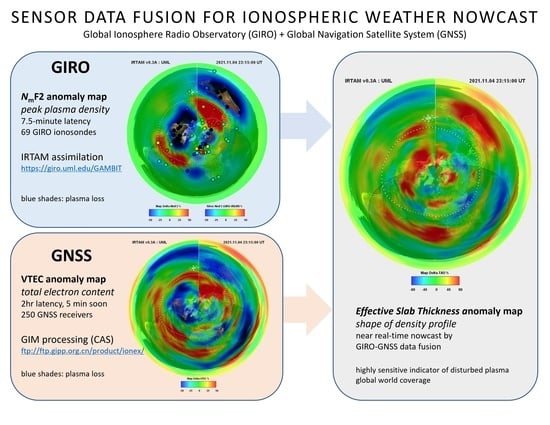
2. GIRO and GNSS for Ionospheric Weather Nowcast

Our choice of GIRO and GNSS sensor networks for monitoring the ionosphere has been driven by the practical considerations described in the previous section. Both networks offer the vital capability of centralized data acquisition within minutes from the observation, an algorithmic suite for extracting useful information from raw measurements, and a robust synthesis engine for generating continuous global maps.

2.1. Ionospheric Weather Nowcast Using GIRO Ionosondes

Figure 1 depicts one of the standard GIRO nowcast products, an anomaly map of MUF for a 3000 km HF communications link, plotted as the “weather-minus-climate” percent deviation of the current ionospheric weather from its expected quiet-time climate reference computed by IRI for the same time. Color dots in Figure 1 correspond to the MUF(3000) weather-minus-climate as observed locally at GIRO ionosonde locations, while the color surface is the global anomaly map computed by the NECTAR algorithm [8] that fuses GIRO data and IRI model [9] for the global coverage. Blue shades in the anomaly map correspond to the MUF depressions that, should they reach at least 30% from the quiet-time expectations, trigger HF communication alerts (e.g., [25]) that might be then followed by safety mitigation measures as harsh as re-routings of transpolar civil aviation flights.

2.2. Ionospheric Weather Nowcast Using GNSS Receiver Network

With the number of online dual-frequency ground-based GNSS receivers exceeding the 20,000 mark and growing, high-resolution VTEC maps can be assembled by simply placing VTEC values at the piercing point locations, without interpolation, covering the essential parts of the globe (Figure 2). Naturally, neither GNSS nor GIRO networks can provide ionosphere coverage over the ocean surfaces where instrument installations are rare, being bound to islands and marine platforms such as buoys and ships [26]. In the absence of sensor measurements, global mapping of the ionospheric weather smoothly returns to the background model of climate specification.

2.3. Anomaly Mapping Using Gleason Projection

In illustrating the combined capability of the networks, we will use the North Polar “Gleason” projection of the globe (Figure 3) [28] instead of the more familiar Mercator or sinusoidal systems (as in Figure 1 and Figure 2).
The North Polar projection has a substantial advantage of continuous visual representation of the ionospheric disturbances without interrupting them at 180° longitude map discontinuity. In this projection, the North pole is placed at the center of the map circle, while the longitude-latitude grid of the globe is gradually stretched as the latitude decreases. The South pole is stretched along the border of the outer circle. The subsolar point is indicated with a Sun symbol, and the night-time area is shadowed. This projection emphasizes the Northern hemisphere, with better ground sensor coverage.
We will use the weather-minus-climate (“anomaly”) maps to compare the GIRO and GNSS capabilities in sensing the ionosphere dynamics. Even though the nature of the ionospheric characteristics may be different in these comparisons, presenting them as the metrics of how different the ionosphere is from its expected quiet-time behavior is helpful in the comparative assessments. The quiet-time climatology reference for the weather-minus-climate computation varies depending on the nature of the map; IRTAM is nominally contrasted to the IRI background, while VTEC can be viewed against a 30-day running average [29] or a quiet day before or after the event.

2.4. GAMBIT: Cooperative GIRO and GNSS Nowcast

The outcome of the cooperative GIRO and GNSS nowcast is called GAMBIT (Global Assimilative Model of Bottomside Ionosphere with a Topside Estimate) [30]. Cross-instrument anomaly mapping by GIRO and GNSS is illustrated in Figure 4. One data frame is selected out of the 4–7 November 2021 G3 storm period, during which several HF communications alerts were issued to civil aviation because of the ongoing MUF depression. Figure 4 compares anomaly reporting capabilities of GIRO (peak density NmF2 in the left panel) and two different GNSS resources (VTEC from CEDAR Madrigal repository and UPC Quarterly Rapid map in the middle and right panels). Note that no interpolation or extrapolation is used to plot VTEC data from the Madrigal collection that features a few thousand receivers and over 12,000 pierce points (the gray color is used to denote no-data areas).
Overall, good qualitative agreement on the negative anomalies that have triggered the flight safety alerts is observed over the North American, Australian, mid-Atlantic, and Siberian sectors on all three panels of Figure 4. Remarkably, though, anomalies in the equatorial regions of South Africa suggest the opposite dynamics: peak density remains low, while both VTEC maps suggest an increased total content. This observation corresponds to a vertically “stretched” F2 ionospheric region with a significant contribution from the topside ionosphere and possibly plasmasphere. Additionally, both GIRO and Quarterly Rapid VTEC maps suggest a pronounced super-fountain event over South America. However, closer inspection of the area in high-resolution VTEC (Figure 5a) reveals a different argument: finely structured signatures of a strong equatorial spread F (ESF) event in progress, confirmed by the directogram measurement [31] by Sao Luis Digisonde (Figure 5b).
All data resources, and NASA WorldWind visualization engine [32], for the GIRO-GNSS cross-instrument percent anomaly mapping are available in the public domain at Lowell GIRO Data Center (LGDC) using GAMBIT Database and Explorer [30]. GAMBIT Explorer uses the Madrigal interface to retrieve VTEC data from MIT Haystack Observatory, Westford, Massachusetts, and 30-day average and Quarterly Rapid VTEC maps are downloaded from the University of Warmia and Mazury (UWM) publishing server in Olsztyn, Poland.

3. Technique Descriptions

The challenge of ionospheric imaging is the multi-faceted wave phenomena affecting the probing signal. These effects must be interpreted intelligently to glean the plasma properties of interest. Unavoidable data noise and bias, significant at times, accompany this interpretation and propagate from the input to the result of the sensor data fusion. Space weather assimilation schemas based on the conventional update-forecast iterative approach are particularly prone to stability issues because of the occasional data blunders at their input.
Sensor data conditioning has become an integral part of fusion systems. We approach the task differently for GIRO and GNSS components of GAMBIT, as explained below.

3.1. GIRO-IRI Data Fusion

The associative restoration of missing, corrupted, deteriorating, or unwanted parts of the 2D imagery has become an essential topic of contemporary computer vision science. Image inpainting [33] is one rapidly developing branch of the domain. Much like NECTAR, image inpainting algorithms smoothly blend missing or removed pixels to an associated trained model of matching content. The model can be built from historical records or gleaned from the neighboring pixels. Unlike typical image inpainting techniques, NECTAR involves additional arguments for the restoration by treating the ionosphere as a medium of particular wave-like, cyclic variability. While the underlying ionospheric climatology model captures the geophysics-motivated description of the global plasma density distribution, current weather processes are presented by NECTAR as deviations from the climate reference described in terms of their temporal diurnal harmonics. Such multi-scale “eigenfunction” treatment highlights the natural constituent processes in the ionosphere that exhibit cyclic behavior of various scales. It also allows for the subsequent spatial interpolation and extrapolation of the data outside GIRO sites to reason about the spatial extent of detected anomalies by observing their temporal features, thus enabling the time-to-space prediction. For example, suppose NECTAR analysis confirms the presence of a strong cyclic anomalous 12-h harmonic at a particular site. In that case, the observed periodicity can be translated to the matching wavelength of the underlying planetary-scale disturbance and extended spatially to the vicinity of the detection point.
IRTAM adds the vertical dimension to the NECTAR-computed 2D surface maps of the peak density NmF2, peak height hmF2, and two profile parameters B0 and B1 by using them as the anchor points of the IRI specification of the 1D vertical profile of the subpeak electron density [9]. By its design, IRTAM falls into the category of so-called 4DVAR assimilation models that include the history of measurements within a certain time window as an additional dimension for their assimilation. Each 4DVAR computation ensures matching of the updated model not only to current but also past observations, in contrast to 3DVAR schemas that update the model only at the analysis time. Although originally “4D” referred to the addition of the time dimension to 3D models of spatial properties such as the electron density Ne, later extensions of the concept included multi-dimensional properties as well. Technically, each NECTAR computation ensures the optimal fit of 24 × 4 = 96 surface maps to the measurements within 24 h before the current time, which would be a “2D + time” assimilation. Perhaps a description of IRTAM as a (2D + time) + 1D assimilative model would be more correct. For simplicity of notation, we will still refer to IRTAM as a 4DVAR model.
The availability of the 24-h analysis window in a single 4DVAR IRTAM calculation afforded stronger conditioning of GIRO data before they enter the assimilation process. While classic uncertainty analysis of the Kalman filter assumes the normal measurement error distribution, 4DVAR allows outlier detection and analysis of the confidence scores of ionogram autoscaling [34] that have strengthened sensor data conditioning GIRO measurements. Further detail and analysis of the NECTAR spatial prediction capability can be found in [8].

3.2. VTEC Maps by IGS/UWM/CAS

The Chinese Academy of Sciences (CAS) started regular releases of Global Ionospheric Maps (GIMs) in 2015. Since then, CAS has become one of IGS’ Ionosphere Associate Analysis Centers (IAACs), providing VTEC maps in their real-time, rapid, and final routines [35]. In general, all these products utilize spherical harmonics [36] in combination with the generalized trigonometric series [37]. While rapid and final products have been made publicly available at the NASA CDDIS archive since January 2010, covering periods since 2015 and 1998, respectively, CAS does not promptly disseminate real-time GIMs, leaving the only data access capability to its FTP repository at ftp://ftp.gipp.org.cn/product/ionex/ (accessed on 9 January 2022) [35]. For optimal GIRO-GNSS fusion, the real-time CAS GIMs are transformed at UWM into the standard NASA WorldWind [32] grid format for GIRO, much like the global climate weather VTEC maps derived from the rapid UPC UQRG product [29].
While accurate measurements of the differential pseudorange and phase of GNSS signals are readily available in the dual-frequency receivers for their conversion to STEC and VTEC, effects other than refraction in plasma introduce additional unknown and varying differential code biases (DCB). The CAS IAAC provides Satellite DCBs from Multi-GNSS Experimental (MGEX) DCB solution [38,39] and receiver DCBs estimated locally using a Modified Generalized Trigonometric Series (MGTS) function [40] to calibrate both types. The next step is to bring multiple available real-time VTEC observations by GPS, GLONASS, BDS, GALILEO, MGEX, and other local networks to their mutual agreement. Such multi-GNSS maps are computed at CAS using the so-called “predicting-plus-modeling” method [40]. To mitigate potential stability problems of the incoming data stream, e.g., its interruptions for technical reasons, computation of CAS RT-GIM involves predicted TEC maps [40] to thus accomplish a nominal stable data latency of about 5 min [35].
The proper data conditioning of the GNSS receiver measurements is crucial for accurate generation and combination of VTEC Global Ionospheric Maps (GIMs) at final, rapid, and real-time (RT) scales. Such treatment of potential sources of data processing errors must be fully automatic. One example is the proper detection of GNSS carrier phase cycle slips [41] and either cycle slip fixing [42,43]. Other examples are the interpolation of directly estimated VTEC values in RT, significantly improving the quality of the RT UPC GIMs [44], and the RT automatic assessment of RT GIMs to generate a better combined RT GIM in IGS [45].

3.3. 2D Versus 3D Modeling of the Ionosphere

While global 2D maps of VTEC have been instrumental in expanding the knowledge base of the ionosphere, much research and many applied space weather interests demand specification of the 3D volume of the ionospheric plasma. The 3D modeling is essential for monitoring HF signal propagation conditions, which necessitates ray-tracing the propagating signal through the plasma layers. Ionosondes readily provide sufficient information on the vertical plasma distribution in the bottomside ionosphere that can be readily assimilated in IRTAM and other 3D models. As for the traversing GNSS signals, computerized ionospheric tomography must be applied to original STEC measurements instead of converted VTEC data to extract the required information.
Three classes of computerized ionospheric tomography techniques have emerged over the years [16,46,47,48,49,50,51,52,53]:
  • Based on solving the inverse problem (via Radon transform for the satellite-to-ground sounding [47,48] or Abel transform for the satellite-to-satellite radio occultation (e.g., [49]),
  • Assimilative models that use acquired STEC data to transform a suitable background plasma density model ([50,51] and others), and
  • Adaptable-resolution models that adjust themselves to the distribution of the measurements, thus avoiding the need for a background model [16,52,53].
The first two classes of tomography solutions were adopted from other disciplines (oceanography, meteorology, and X-ray radiography) to solve a much more complicated task of the ionospheric specification that is underdetermined and ill-posed by its definition [54]. The techniques had to be extensively improved for the task and enhanced with sensor fusion complements [16,50,55]. Simultaneous assimilation of the GIRO and GNSS measurements into the same computational schema such as the IRI model tends to be inefficient: the much wider availability of GNSS receivers results in merely adding GIRO sensor data to the mix. Efforts to improve the accuracy of the bottomside ionosphere description for demanding projects such as geolocation of ground HF emitters [24,25] led to solutions where STEC data are weighted down for assimilation or even not assimilated at all, to give preference to other sensors of higher accuracy or relevance. However, there is one easy possibility of fusing GIRO and GNSS domains that we are exploring.

4. Fusing GIRO and GNSS Data

Visual inspection of the 2D anomaly maps of NmF2 versus VTEC (as in Figure 4) may suggest that observed delta-VTEC features may be simply duplicated and then suitably superimposed and blended with the NmF2 map, thus accomplishing its better resolution and additional coverage of missing data. Statistically, variation of VTEC was indeed reported, often matching that of NmF2 (e.g., [56] and references therein). However, up to 50% of the VTEC must be attributed to the plasmasphere content above the ionosphere [57], which introduces significant and, in many cases, unacceptable uncertainty regarding whether such direct attribution of delta-VTEC to delta-NmF2 is realistic. Furthermore, neither peak height hmF2 nor profile shape parameters B0 and B1 can be obtained directly from 2D VTEC maps.
Instead, readily available global real-time maps of NmF2 and VTEC can be used to obtain an important property of the total shape of the vertical profile of electron density, the ionospheric Equivalent Slab Thickness (EST).

4.1. Equivalent Slab Thickness Computation

The ionospheric Equivalent Slab Thickness τ is defined as a ratio of the vertical total electron content to the F2 layer peak electron density [58,59]:
τ = VTEC/NmF2
where the vertical TEC is given in TEC units (electrons per m2), NmF2 is in electrons per m3, and τ is in meters. EST is an important parameter of an imaginary ionosphere with the same TEC as the actual ionosphere and a constant uniform density equal to NmF2. In other words, τ represents the equivalent slab thickness/depth of an idealized ionosphere with the same electron content as the actual ionosphere but with uniform electron density equal to the maximum electron density [60].

4.2. Importance of EST for Monitoring the Ionosphere

Fundamentally, τ extracts new information from two independent measurement resources that is not readily deducible from either resource alone [61]. The new information enhances each resource: the total electron content is now provided with a certain understanding of the profile shape, while the bottomside density specification is now accompanied by a certain characterization of the supra-peak plasma. The importance of such τ computation has been recognized in different applied and academic domains, ranging from planning and operation of spacecraft navigation and communication systems, where EST improves understanding of the temporal and spatial behavior of TEC [62], to model development and validation [63,64], where the ingestion of EST observations can reveal weaknesses in the model EST estimation (by comparing the model-retrieved NmF2 values with the experimental ones).
In addition to the capability of τ to characterize the overall shape of Ne(h) profile, multiple authors confirm EST as an efficient and consistent proxy to various underlying physical processes in the ionosphere and plasmasphere, including ionization efficiency and plasma transport, with peculiar diurnal patterns and seasonal behavior that can shed light even on dynamics of the solar input at the top of the ionosphere:
  • τ has been linked to the neutral scale height Hn of the atmosphere [58] according to the relation τ = 4.13 Hn. This relation has been recently re-confirmed as valid, even though only for the α-Chapman function representation of the F2 layer of the ionosphere under strict assumptions [65] that have not been fully met in real life. The vertical distribution of the ionospheric plasma is instead driven by the plasma scale height Hp, which depends on the plasma temperature, ion composition, and other physical quantities [66]. Correspondingly, this relationship with Hn is now viewed as a benchmark [67].
  • A rough estimate of the thermospheric temperature Tn can be obtained as a function of τ [68]: Tn = (τ + 250)/0.5.
  • Statistical associations of τ with seasonal and solar activity variability are instrumental to understanding its relationship with the forcing from above. Global climatological and weather modeling [68,69] highlights good correlations of τ with solar heat input unless dominating plasma transport processes break the equilibrium conditions.

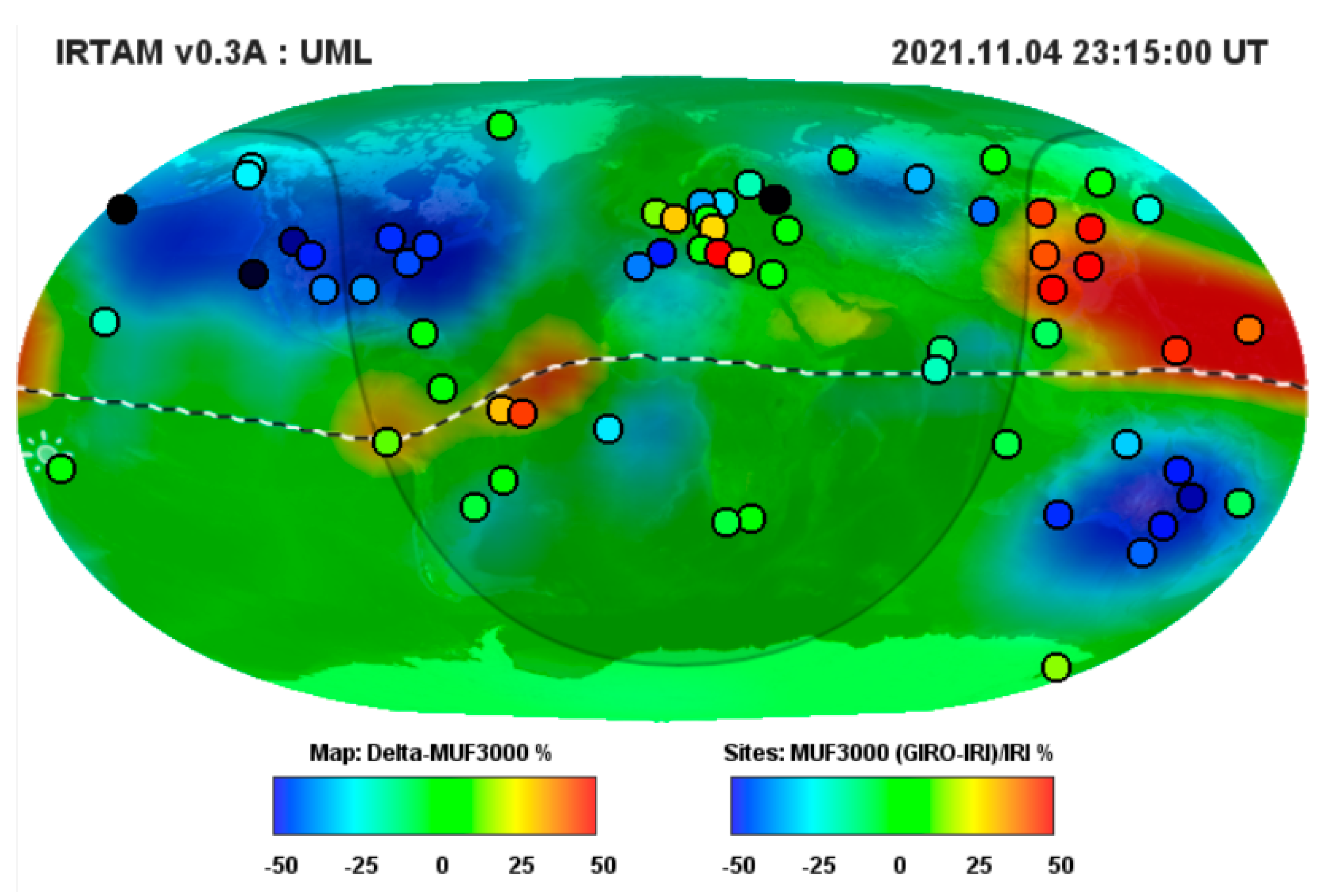
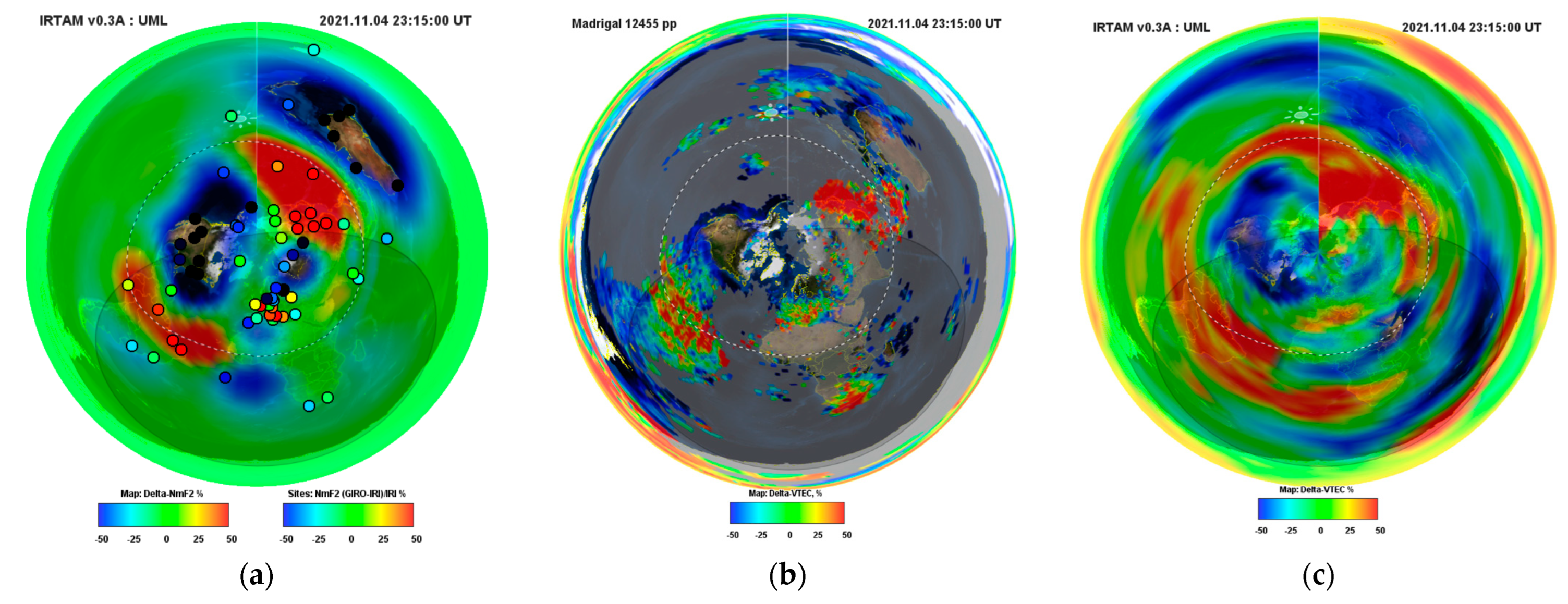
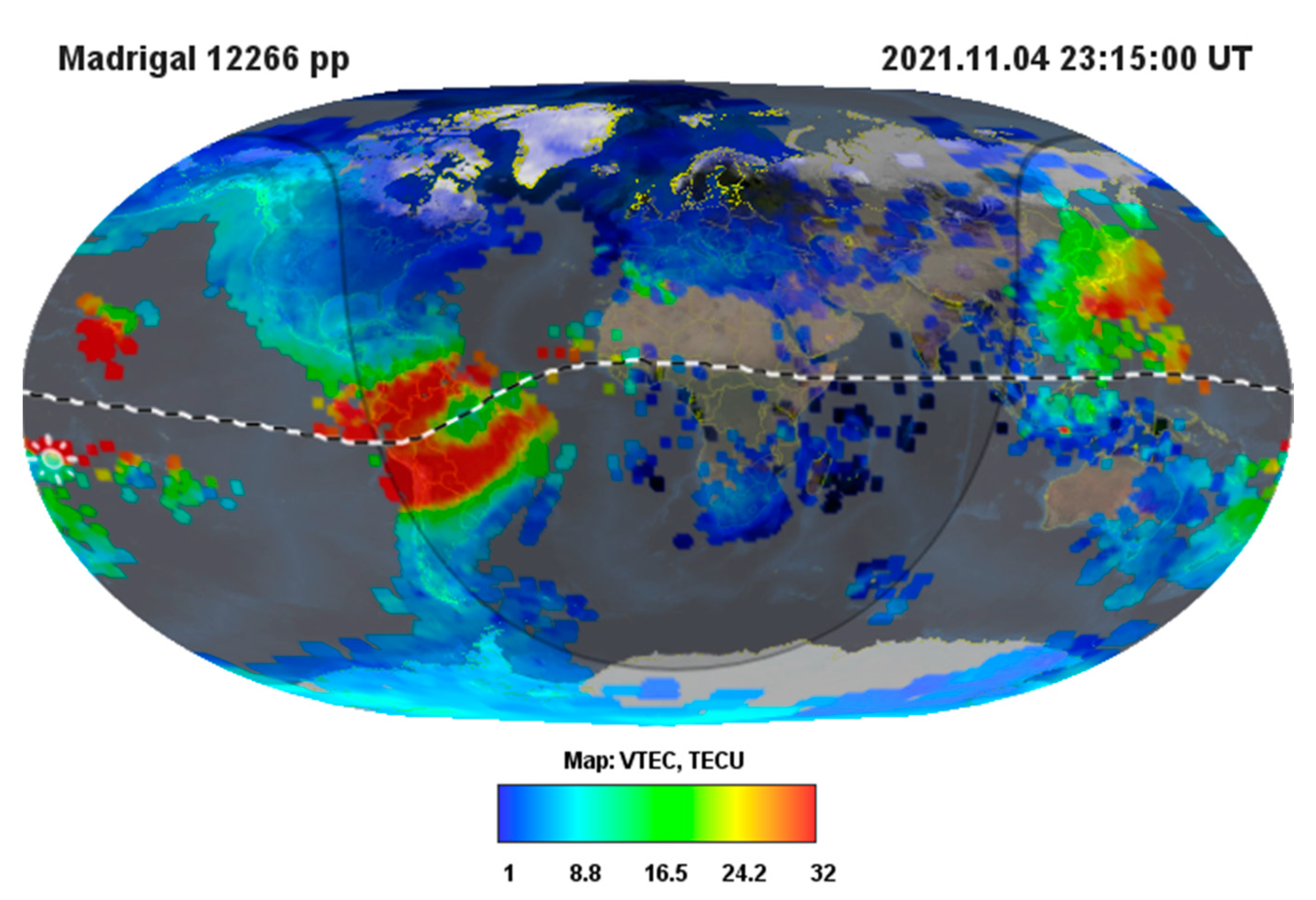
4.3. EST: 4 November 2021 Case Study

Figure 6a presents real-time EST computation for the 4 November 2021, 23:15UT case of the G3-category storm (the left panel). It is not easy to distinguish anomalous features by just analyzing the global EST map alone: it still features commonly observed patterns [29], e.g., a remarkable pre-sunrise increase above 800 km due to the ionosphere topside being lit by the Sun ahead of the lower layers. It is the capability of referencing the weather map against the quiet-time background (Figure 6b) that highlights substantial >80% enhancements over the four areas of NmF2 depression seen in Figure 4.
Remarkably, detected global-scale anomalies of the τ distribution seen in Figure 6b are expressed significantly more strongly than their constituent anomalies of NmF2 and VTEC in Figure 4 or the MUF(3000) property of HF communications in Figure 1. Such sensitivity to abnormal processes in the ionosphere makes the effective slab thickness a good candidate for weather monitoring and alerts.

5. Summary and Future Work

Unlike the first decades of exploring the ionosphere, modern ionospheric monitoring is no longer about extending the body of empirical knowledge; it is about alerting the impacted operational systems that employ trans-ionospherically propagating signals. Proper monitoring is now fully automatic and prompt; it is the last resort to inform end-users of an ongoing anomaly during those times and locations when and where the predicted behavior of the ionosphere did not match the reality. Correspondingly, it is designed and built as glass-room weather service, with suitable low-latency sensor instrumentation, automated extraction of actionable information from the real-time streaming sensor data, and 3D plasma modeling algorithms robust to potential data noise and bias at their input.
Sensor data fusion remains a practical requirement of modern ionospheric monitoring as the 3D specification of the ionospheric plasma requires populating the vast spaces of the near-Earth environment with sensors, which is still impractical without collaboration. Developing a data-fused GIRO and GNSS weather service is our first step towards the aforementioned objectives. The current scenario involves the Lowell GIRO Data Center, which operates the IRTAM 3D assimilative model and a consortium of IGS coordination centers in Poland, Spain, and China that have ultra-rapid quarterly VTEC mapping capability. Monitoring the effective slab thickness of the ionosphere is one immediate outcome of this collaboration, with clear benefits of characterizing properties of the geospace above ionospheric peak height using solely ground-based remote sensing resources.
Further steps toward collaborative imaging of the ionosphere will likely involve ultraviolet spectrographs with the capability of sensing the plasma density, such as GOLD [70,71], and spacecraft-to-spacecraft Radio Occultation (RO) networks, such as SPIRE [72] and FORMOSAT-7/COSMIC-2 [73]. Although practical considerations of the high expense of RT telemetry downlink delay the availability of RO measurements by as much as 2 h, new machine learning capabilities are emerging for ionospheric weather forecasting [74] that may satisfy the accuracy requirements of most applications.

Author Contributions

Conceptualization: I.G. and A.K; Methodology: I.G., A.K., M.H.-P., B.N., D.B., and B.R.; Software: I.G., A.F., K.K., and P.F.; Validation: A.F., A.K., I.G., and D.B.; Formal analysis: I.G., A.K., A.F., and D.B.; Investigation, resources, and data curation: I.G., M.H.-P., A.F., Z.L., N.W., K.K., P.F., D.R.D., A.G.-R., and I.B.; Writing—original draft preparation: I.G., M.H.-P., B.N., A.K., and D.B.; Writing—review and editing: I.G., D.B., and B.R.; Visualization: I.G.; Supervision: I.G., A.K., D.B., and B.R.; Project administration: B.R., A.K., and I.G.; Funding acquisition: A.K. and I.G. All authors have read and agreed to the published version of the manuscript.

Funding

The UML contribution is supported by GAMBIT Situation Room subscription fees. The UWM contribution is supported by the National Centre for Research and Development, Poland, through grant ARTEMIS (decision numbers DWM/PL-CHN/97/2019 and WPC1/ARTEMIS/2019) and the National Science Centre, Poland, through grant 2017/27/B/ST10/02190. The UWM authors also thank the Ministry of Education and Science (MES), Poland for granting funds for the Polish contribution to the International LOFAR Telescope (agreement no. 2021/WK/02). The UPC-IonSAT authors also thank the support of the European-Union-funded project PITHIA-NRF (grant no. 101007599).

Institutional Review Board Statement

Not applicable.

Informed Consent Statement

Not applicable.

Data Availability Statement

Publicly available datasets were analyzed in this study. All datasets are available for download and visualization using the GAMBIT Explorer application, found here: https://giro.uml.edu/GAMBIT (accessed on 9 January 2022). Contributing online data repositories used by GAMBIT Explorer are (1) Lowell GIRO Data Center, (2) NSF CEDAR Madrigal Data node at MIT Haystack Observatory, and (3) IGS VTEC weather and climate data repository operated by UWM.

Acknowledgments

We thankfully acknowledge the contribution of data from 69 operators of ionosondes worldwide to the GIRO server at UML and from the many GNSS ground-station operators to the GNSS data analysis centers and the International GNSS Service (IGS) of ionospheric data.

Conflicts of Interest

The authors declare no conflict of interest. The funders had no role in the study’s design, in the collection, analyses, or interpretation of data, in the writing of the manuscript; or in the decision to publish the results.

References

  1. Gilliland, T.R.; Kenrick, G.W. Preliminary note on an automatic recorder giving a continuous height record of the Kennelly-Heaviside layer. Proc. Inst. Radio Eng. 1932, 20, 540–547. [Google Scholar] [CrossRef]
  2. Daniell, R.E.; Decker, D.T.; Anderson, D.N.; Jaspers, J.R.; Sojka, J.J.; Schunk, R.W. A global ionospheric conductivity and electron density (ICED) model. In Proceedings of the Ionospheric Effects Symposium, Alexandria, VA, USA, 1–3 May 1990. [Google Scholar]
  3. Daniell, R.E.; Whartenby, W.G.; Brown, L.D. Parameterised Real-Time Ionospheric Specification Model, PRISM Version 1.2; Computational Physics: Newton, MA, USA, 1993. [Google Scholar]
  4. Buchau, J.; Bullett, T.W.; Ronn, A.E.; Scro, K.D.; Carson, J.L. The Digital Ionospheric Sounding System Network of the US Air Force Weather Service; Report UAG-104, WDC-A for Solar-Terrestrial Physics; Ionosonde Network Advisory Group: Boulder, CO, USA, 1995; pp. 16–20. [Google Scholar]
  5. Bibl, K.; Reinisch, B.W. The universal digital ionosonde. Radio Sci. 1985, 13, 519–530. [Google Scholar] [CrossRef]
  6. Reinisch, B.W.; Huang, X. Automatic calculation of electron density profiles from digital ionograms: 3. Processing of bottomside ionograms. Radio Sci. 1983, 18, 477–492. [Google Scholar] [CrossRef]
  7. Reinisch, B.W.; Galkin, I.A. Global ionospheric radio observatory (GIRO). Earth Planet. Sci. 2011, 63, 377–381. [Google Scholar] [CrossRef] [Green Version]
  8. Galkin, I.A.; Reinisch, B.W.; Vesnin, A.M.; Bilitza, D.; Fridman, S.; Habarulema, J.B.; Veliz, O. Assimilation of Sparse Continuous Near-Earth Weather Measurements by NECTAR Model Morphing. Space Weather 2020, 18, e2020SW002463. [Google Scholar] [CrossRef]
  9. Bilitza, D.; Altadill, D.; Truhlik, V.; Shubin, V.; Galkin, I.A.; Reinisch, B.W.; Huang, X. International Reference Ionosphere 2016: From ionospheric climate to real-time weather predictions. Space Weather 2017, 15, 418–429. [Google Scholar] [CrossRef]
  10. Galkin, I.A.; Reinisch, B.W.; Huang, X.; Bilitza, D. Assimilation of GIRO Data into a Real-Time IRI. Radio Sci. 2012, 47, RS0L07. [Google Scholar] [CrossRef]
  11. Galkin, I.A.; Reinisch, B.W.; Bilitza, D. Realistic Ionosphere: Real-time ionosonde service for ISWI. Sun Geosph. 2018, 13, 173–178. [Google Scholar]
  12. Mannucci, A.J.; Wilson, B.D.; Yuan, D.N.; Ho, C.H.; Lindqwister, U.J.; Runge, T.F. A global mapping technique for GPS-derived ionospheric total electron content measurements. Radio Sci. 1998, 33, 565–582. [Google Scholar] [CrossRef]
  13. Klobuchar, J.A. Ionospheric Time-Delay Algorithm for Single-Frequency GPS Users. IEEE Trans. Aerosp. Electron. Syst. 1987, 3, 325–331. [Google Scholar] [CrossRef]
  14. Hajj, G.A.; Romans, L.J. Ionospheric electron density profiles obtained with the Global Positioning System: Results from the GPS/MET experiment. Radio Sci. 1998, 33, 175–190. [Google Scholar] [CrossRef] [Green Version]
  15. Hernández-Pajares, M.; Juan, J.M.; Sanz, J. Improving the Abel inversion by adding ground GPS data to LEO radio occultations in ionospheric sounding. Geophys. Res. Lett. 2000, 27, 2473–2476. [Google Scholar] [CrossRef] [Green Version]
  16. Hernández-Pajares, M.; Juan, J.M.; Sanz, J.; Solé, J.G. Global observation of the ionospheric electronic response to solar events using ground and LEO GPS data. J. Geophys. Res. Space Phys. 1998, 103, 20789–20796. [Google Scholar] [CrossRef] [Green Version]
  17. Fung, S.F.; Benson, R.F.; Galkin, I.A.; Green, J.L.; Reinisch, B.W.; Song, P.; Sonwalker, V. Chapter 4—Radio-frequency imaging techniques for ionospheric, magnetospheric, and planetary studies. In Magnetospheric Imaging: Understanding the Space Environment through Global Measurements; Colado-Vega, Y., Gallagher, D., Frey, H., Wing, S., Eds.; Elsevier: Amsterdam, The Netherlands, 2022; pp. 101–216. [Google Scholar]
  18. Kiselyova, M.V.; Kijanowski, M.P.; Knyazuyk, V.S.; Lyakhova, L.N.; Yudovich, L.A. Forecast of the F2 layer critical frequency. In Ionospheric Disturbances and Their Impact on Radio Communications; Nauka: Moscow, Russia, 1971; pp. 74–99. (In Russian) [Google Scholar]
  19. Kotonaeva, N.G.; Kolomin, M.V.; Mikhailov, V.V.; Tsybulya, K.G.; Philippov, M.Y. Efficiency of ionospheric model correction by vertical-incidence sounding data from an ionosonde during low sunspot activity. Geomagn. Aeron. 2022, 61, 92–99. [Google Scholar] [CrossRef]
  20. Rabier, F. Overview of global data assimilation developments in numerical weather-prediction centres. Q. J. R. Meteorol. Soc. 2005, 131, 3215–3233. [Google Scholar] [CrossRef]
  21. McNamara, L.F.; Wilkinson, P.J. Spatial correlations of foF2 deviations and their implications for global ionospheric models: 1. Ionosondes in Australia and Papua New Guinea. Radio Sci. 2009, 44, RS2016. [Google Scholar] [CrossRef]
  22. McNamara, L.F. Spatial correlations of foF2 deviations and their implications for global ionospheric models: 2. Digisondes in the United States, Europe, and South Africa. Radio Sci. 2009, 44, RS2017. [Google Scholar] [CrossRef]
  23. Harón, S.; Prasanth, R.; Raz, G.; McClure, M.; Titi, G.; Li, J.; Xu, L. HFGeo signal processing and channel modeling. In Proceedings of the 2015 Ionospheric Effects Symposium, Alexandria, VA, USA, 12–14 May 2015. [Google Scholar]
  24. Mitchell, C.N.; Rankov, N.R.; Bust, G.S.; Miller, E.; Gaussiran, T.; Calfas, R.; Doyle, J.D.; Teig, J.D.; Werth, J.L.; Dekine, I. Ionospheric data assimilation applied to HF geolocation in the presence of traveling ionospheric disturbances. Radio Sci. 2017, 52, 829–840. [Google Scholar] [CrossRef] [Green Version]
  25. Sabbagh, D.; Bagiacchi, P.; Scotto, C. Accuracy assessment of the MUF(3000) nowcasting for PECASUS space weather services. In Proceedings of the 23rd URSI General Assembly and Scientific Symposium, Rome, Italy, 29 August–5 September 2020. [Google Scholar]
  26. Azeem, I.; Crowley, G.; Forsythe, V.V.; Reynolds, A.S.; Stromberg, E.M.; Wilson, G.R.; Kohler, C.A. A new frontier in ionospheric observations: GPS total electron content measurements from ocean buoys. Space Weather 2020, 18, e2020SW002571. [Google Scholar] [CrossRef]
  27. Rideout, W.; Coster, A. Automated GPS processing for global total electron content data. GPS Solut. 2006, 10, 219–228. [Google Scholar] [CrossRef]
  28. Gleason, A. Time-Chart. U.S. Patent 497,917, 23 May 1893. Available online: https://patents.google.com/patent/US497917A/en (accessed on 6 January 2022).
  29. Froń, A.; Galkin, I.A.; Krankowski, A.; Bilitza, D.; Hernández-Pajares, M.; Reinisch, B.; Li, Z.; Kotulak, K.; Zakharenkova, I.; Cherniak, I.; et al. Towards Cooperative Global Mapping of the Ionosphere: Fusion Feasibility for IGS and IRI with Global Climate VTEC Maps. Remote Sens. 2020, 12, 3531. [Google Scholar] [CrossRef]
  30. Global Assimilative Model of Bottomside Ionosphere Timeline (GAMBIT). Available online: https://giro.uml.edu/GAMBIT (accessed on 6 January 2022).
  31. Reinisch, B.W.; Galkin, I.A.; Khmyrov, G.M.; Kozlov, A.V.; Bibl, K.; Lisysyan, I.A.; Cheney, G.P.; Huang, X.; Kitrosser, D.F.; Paznukhov, V.V.; et al. New Digisonde for research and monitoring applications. Radio Sci. 2009, 44, RS0A24. [Google Scholar] [CrossRef]
  32. NASA WorldWind. Available online: https://worldwind.arc.nasa.gov (accessed on 6 January 2022).
  33. Guillemot, C.; Le Meur, O. Image Inpainting: Overview and Recent Advances. IEEE Signal Process. Mag. 2014, 31, 127–144. [Google Scholar] [CrossRef]
  34. Galkin, I.A.; Reinisch, B.W.; Huang, X.; Khmyrov, G.M. Confidence score of ARTIST-5 ionogram autoscaling. In Ionosonde Network Advisory Group (INAG) Bulletin No. 73; URSI Secretariat, Commission G: Ghent, Belgium, 2013; pp. 1–7. Available online: http://www.ursi.org/files/CommissionWebsites/INAG/web-73/confidence_score.pdf (accessed on 9 January 2022).
  35. Li, Z.; Wang, N.; Liu, A.; Yuan, Y.; Wang, N.; Hernandez-Pajares, M.; Krankowski, A.; Yuan, H. Status of CAS global ionospheric maps after the maximum of solar cycle 24. Satell. Navig. 2021, 2, 1–15. [Google Scholar] [CrossRef]
  36. Li, Z.; Yuan, Y.; Wang, N.; Hernandez-Pajares, M.; Huo, X. SHPTS: Towards a new method for generating precise global ionospheric TEC map based on spherical harmonics and generalized trigonometric series functions. J. Geod. 2015, 89, 331–345. [Google Scholar] [CrossRef]
  37. Yuan, Y.; Ou, J. A generalized trigonometric series function model for determining ionospheric delay. Prog. Nat. Sci. 2004, 14, 1010–1014. [Google Scholar] [CrossRef]
  38. Wang, N.; Li, Z.; Montenbruck, O.; Tang, C. Quality assessment of GPS, Galileo and BeiDou-2/3 satellite broadcast group delays. Adv. Space Res. 2019, 64, 1764–1779. [Google Scholar] [CrossRef]
  39. Wang, N.; Li, Z.; Duan, B.; Hugentobler, U.; Wang, L. GPS and GLONASS observable-specific code bias estimation: Comparison of solutions from the IGS and MGEX networks. J. Geod. 2020, 94, 74. [Google Scholar] [CrossRef]
  40. Li, Z.; Wang, N.; Hernández-Pajares, M.; Yuan, Y.; Krankowski, A.; Liu, A.; Zha, J.; García-Rigo, A.; Roma-Dollase, D.; Yang, H.; et al. IGS real-time service for global ionospheric total electron content modeling. J. Geod. 2020, 94, 1–16. [Google Scholar] [CrossRef]
  41. Blewitt, G. An automatic editing algorithm for GPS data. Geophys. Res. Lett. 1990, 17, 199–202. [Google Scholar] [CrossRef] [Green Version]
  42. Hernández-Pajares, M.; Roma-Dollase, D.; Garcia-Fernàndez, M.; Orus-Perez, R.; García-Rigo, A. Precise ionospheric electron content monitoring from single-frequency GPS receivers. GPS Solut. 2018, 22, 1–13. [Google Scholar] [CrossRef] [Green Version]
  43. Zhao, J.; Hernández-Pajares, M.; Li, Z.; Wang, L.; Yuan, H. High-rate Doppler-aided cycle slip detection and repair method for low-cost single-frequency receivers. GPS Solut. 2020, 24, 1–13. [Google Scholar] [CrossRef]
  44. Yang, H.; Monte-Moreno, E.; Hernández-Pajares, M.; Roma-Dollase, D. Real-time interpolation of global ionospheric maps by means of sparse representation. J. Geod. 2021, 95, 1–20. [Google Scholar]
  45. Liu, Q.; Hernández-Pajares, M.; Yang, H.; Monte-Moreno, E.; Roma-Dollase, D.; García-Rigo, A.; Li, Z.; Wang, N.; Laurichesse, D.; Blot, A.; et al. The cooperative IGS RT-GIMs: A reliable estimation of the global ionospheric electron content distribution in real time. Earth Syst. Sci. Data 2021, 13, 4567–4582. [Google Scholar] [CrossRef]
  46. Bust, G.S.; Mitchell, C.N. History, current state, and future directions of ionospheric imaging. Rev. Geophys. 2008, 46, 1–23. [Google Scholar] [CrossRef]
  47. Austen, J.R.; Franke, S.J.; Liu, C.H. Ionospheric imaging using computerized tomography. Radio Sci. 2008, 23, 299–307. [Google Scholar] [CrossRef]
  48. Kunitsyn, V.E.; Tereshchenko, E.D. Radio tomography of the ionosphere. IEEE Antennas Propag. Mag. 1992, 34, 22–32. [Google Scholar] [CrossRef]
  49. Schreiner, W.; Sokolovskiy, S.; Rocken, C.; Hunt, D. Analysis and validation of GPS/MET radio occultation data in the ionosphere. Radio Sci. 1999, 34, 949–966. [Google Scholar] [CrossRef]
  50. Fridman, S.V.; Nickisch, L.J.; Hausman, M.; Zunich, G. Assimilative model for ionospheric dynamics employing delay, Doppler, and direction of arrival measurements from multiple HF channels. Radio Sci. 2016, 51, 176–183. [Google Scholar] [CrossRef] [Green Version]
  51. Bruno, J.; Mitchell, C.N.; Bolmgren, K.H.A.; Witvliet, B.A. A realistic simulation framework to evaluate ionospheric tomography. Adv. Space Res. 2020, 65, 891–901. [Google Scholar] [CrossRef]
  52. Hernández-Pajares, M.; Juan, J.M.; Sanz, J. Neural network modeling of the ionospheric electron content at global scale using GPS data. Radio Sci. 1997, 32, 1081–1089. [Google Scholar] [CrossRef] [Green Version]
  53. Hernández-Pajares, M.; Lyu, H.; Garcia-Fernandez, M.; Orus-Perez, R. A new way of improving global ionospheric maps by ionospheric tomography: Consistent combination of multi-GNSS and multi-space geodetic dual-frequency measurements gathered from vessel-, LEO- and ground-based receivers. J. Geod. 2020, 94, 1–16. [Google Scholar] [CrossRef]
  54. Garcia, R.; Crespon, F. Radio tomography of the ionosphere: Analysis of an underdetermined, ill-posed inverse problem, and regional application. Radio Sci. 2008, 43, RS2014. [Google Scholar] [CrossRef] [Green Version]
  55. Angling, M.J.; Jackson-Booth, N.K. A short note on the assimilation of collocated and concurrent GPS and ionosonde data into the Electron Density Assimilative Model. Radio Sci. 2011, 46, RS0D13. [Google Scholar] [CrossRef] [Green Version]
  56. Kotova, D.S.; Ovodenko, V.B.; Yasyukevich, Y.V.; Klimenko, M.V.; Ratovsky, K.G.; Mylnikova, A.A.; Andreeva, E.S.; Kozlovsky, A.E.; Korenkova, N.A.; Nesterov, I.A.; et al. Efficiency of updating the ionospheric models using total electron content at mid- and sub-auroral latitudes. GPS Solut. 2020, 24, 1–10. [Google Scholar] [CrossRef]
  57. Klimenko, M.V.; Klimenko, V.V.; Zakharenkova, I.E.; Cherniak, I.V. The global morphology of the plasmaspheric electron content during Northern winter 2009 based on GPS/COSMIC observation and GSM TIPmodel results. Adv. Space Res. 2015, 55, 2077–2085. [Google Scholar] [CrossRef]
  58. Titheridge, J.E. The slab thickness of the mid-latitude ionosphere. Planet Space Sci. 1973, 21, 1775–1793. [Google Scholar] [CrossRef]
  59. Davies, K. Ionospheric Radio; Peter Peregrinus, Ltd.: London, UK, 1990. [Google Scholar]
  60. Stankov, S.M.; Warnant, R. Ionospheric slab thickness—Analysis, modelling and monitoring. Adv. Space Res 2009, 44, 1295–1303. [Google Scholar] [CrossRef]
  61. Stankov, S.M.; Jakowski, N. Topside ionospheric scale height analysis and modelling based on radio occultation measurements. J. Atmos. Sol. Terr. Phys. 2006, 68, 134–162. [Google Scholar] [CrossRef]
  62. Leitinger, R.; Ciraolo, L.; Kersley, L.; Kouris, S.S.; Spalla, P. Relations between electron content and peak density: Regular and extreme behaviour. Ann. Geophys. 2004, 47, 1093–1107. [Google Scholar]
  63. Nava, B.; Radicella, S.M.; Azpilicueta, F. Data ingestion into NeQuick 2. Radio Sci. 2011, 46, RS0D17. [Google Scholar] [CrossRef] [Green Version]
  64. Migoya-Orué, Y.; Nava, B.; Radicella, S.M.; Alazo-Cuartas, K. GNSS derived TEC data ingestion into IRI 2012. Adv. Space Res. 2015, 55, 1994–2002. [Google Scholar] [CrossRef]
  65. Pignalberi, A.; Nava, B.; Pietrella, M.; Cesaroni, C.; Pezzopane, M. Mid-latitude climatology of the ionospheric equivalent slab thickness over two solar cycles. J. Geod. 2021, 95, 1–18. [Google Scholar] [CrossRef]
  66. Pignalberi, A.; Pezzopane, M.; Nava, B.; Coïsson, P. On the link between the topside ionospheric effective scale height and the plasma ambipolar diffusion, theory and preliminary results. Sci. Rep. 2020, 10, 17541. [Google Scholar] [CrossRef] [PubMed]
  67. Jakowski, N.; Hoque, M.; Mielich, J.; Hall, C. Equivalent slab thickness of the ionosphere over Europe as an indicator of long-term temperature changes in the thermosphere. J. Atm. Sol. Terr. Phys. 2017, 163, 91–102. [Google Scholar] [CrossRef]
  68. Fox, M.W.; Mendillo, M.; Klobuchar, J.A. Ionospheric equivalent slab thickness and its modeling applications. Radio Sci. 1991, 26, 429–438. [Google Scholar] [CrossRef]
  69. Jakowski, N.; Hoque, M.N. Global equivalent slab thickness model of the Earth’s ionosphere. J. Space Weather Space Clim. 2021, 11, 10. [Google Scholar] [CrossRef]
  70. Cai, X.; Burns, A.G.; Wang, W.; Coster, A.; Qian, L.; Liu, J.; Solomon, S.C.; Eastes, R.W.; Daniell, R.E.; McClintock, W.E. Comparison of GOLD nighttime measurements with total electron content: Preliminary results. J. Geophys. Res. Space Phys. 2020, 125, e2019JA027767. [Google Scholar] [CrossRef]
  71. Eastes, R.W.; Solomon, S.C.; Daniell, R.E.; Anderson, D.N.; Burns, A.G.; England, S.L. Global-scale observations of the equatorial ionization anomaly. Geophys. Res. Lett. 2019, 46, 9318–9326. [Google Scholar] [CrossRef] [Green Version]
  72. Angling, M.J.; Nogués-Correig, O.; Nguyen, V.; Vetra-Carvalho, S.; Bocquet, F.-X.; Nordstrom, K.; Melville, S.E.; Savastano, G.; Mohanty, S.; Masters, D. Sensing the ionosphere with the Spire radio occultation constellation. J. Space Weather Space Clim. 2021, 11, 56. [Google Scholar] [CrossRef]
  73. Pedatella, N.M.; Zakharenkova, I.; Braun, J.J.; Cherniak, I.; Hunt, D.; Schreiner, W.S.; Straus, P.R.; Valant-Weiss, B.L.; Vanhove, T.; Weiss, J.; et al. Processing and validation of FORMOSAT-7/COSMIC-2 GPS total electron content observations. Radio Sci. 2021, 56, e2021RS007267. [Google Scholar] [CrossRef]
  74. HRIDE: High Resolution Ionospheric Data Exploitation for Autonomous Vehicle Safety and Operations and Earthquake Precursor Detection. ESA Demonstration Project. 2021. Available online: https://business.esa.int/projects/hride (accessed on 9 January 2022).
Figure 1. GIRO weather nowcast showing a severe ~50% depression of the Maximum Usable Frequency (MUF) (blue shades) during a negative phase of the 4−7 November 2021 G3−category storm. Color dots: local deviations of MUF from the quiet-time International Reference Ionosphere (IRI) model as observed by 67 GIRO ionosondes. Color surface: global MUF anomaly map computed by GIRO-IRI data fusion algorithm NECTAR. The dashed line is the magnetic equator, and the shaded area corresponds to nighttime.
Atmosphere 13 00371 g001
Figure 2. Global high-resolution Vertical TEC map produced using individual GNSS VTEC values at 12,266 pierce points by 4911 receivers (courtesy MIT Madrigal database [27]). The gray color denotes areas of missing sensor coverage; the dashed line is the magnetic equator; the shaded area is nighttime.
Atmosphere 13 00371 g002
Figure 3. North Polar Gleason projection for the 2D Earth maps. The dashed line is the magnetic equator, and the shaded area corresponds to nighttime.
Atmosphere 13 00371 g003
Figure 4. Weather−minus−climate percent anomaly maps showing plasma density depression on November 4, 2021, 23:15 UT as seen by GIRO and GNSS. (a) GIRO ΔNmF2 map, 7.5−min latency, and 69 sites. (b) Madrigal ΔVTEC, several days latency, and 4911 sites. (c) UPC Rapid ΔVTEC map, 2 h latency, 5 min soon, and 250 sites. The dashed line is the magnetic equator, and the shaded area corresponds to nighttime.
Atmosphere 13 00371 g004
Figure 5. Low-latitude American sector anomaly during November 4, 2021, 23:15 UT. (a) Comparative study of the GIRO peak density ΔNmF2 (color dots) and GNSS total content ΔVTEC (color surface) against the 30 October 2021, quiet-time reference. The dashed line is the magnetic equator. (b) Sao Luis Digisonde directogram showing an intense equatorial spread F event in progress. Dashed lines: ionization bubbles drifting across the station eastward (blue color) and westward (red color).
Atmosphere 13 00371 g005
Figure 6. Global maps of effective slab thickness: (a) weather nowcast of EST using coordinated GIRO and GNSS capability, and (b) EST “anomaly” map of deviations from the quiet−time expected behavior. The dashed line is the magnetic equator, and the shaded area corresponds to nighttime.
Atmosphere 13 00371 g006
Publisher’s Note: MDPI stays neutral with regard to jurisdictional claims in published maps and institutional affiliations.

