Article

Intra-Seasonal and Intra-Annual Variation of the Latent Heat Flux Transfer Coefficient for a Freshwater Lake

1
Department of Hydraulic and Water Resources Engineering, Faculty of Civil Engineering, Budapest University of Technology and Economics, H-1111 Budapest, Hungary
2
Department of Meteorology, Institute of Geography and Geosciences, Eötvös Loránd University, H-1117 Budapest, Hungary
*
Author to whom correspondence should be addressed.
Atmosphere 2022, 13(2), 352; https://doi.org/10.3390/atmos13020352
Submission received: 21 December 2021 / Revised: 28 January 2022 / Accepted: 13 February 2022 / Published: 19 February 2022
(This article belongs to the Special Issue Eddy Covariance Methodology for Carbon, Water and Energy Exchanges)

Abstract

:
In the case of lakes, evaporation is one of the most significant losses of water and energy. Based on high-frequency eddy-covariance (EC) measurements between May and September of 2019, the offshore heat and water vapor exchanges are evaluated for the large (~600 km2) but shallow (~3.2 m deep) Lake Balaton (Transdanubian region, Hungary). The role of local driving forces of evaporation in different time scales (from 20 min to one month) is explored, such as water surface and air temperatures, humidity, atmospheric stability, net radiation, and energy budget components. EC-derived water vapor roughness lengths and transfer coefficients (Cq) show an apparent intra-seasonal variation. Different energy balance-based evaporation estimation methods (such as the Priestley-Taylor and the Penman-Monteith) confirm this observation. Furthermore, this has suggested the existence of an intra-annual variation in these parameters. This hypothesis is verified using ten years of water balance measurements, from which, as a first step, evaporation rates and, second, transfer coefficients are derived on a monthly scale. Cq is highly reduced in winter months (~1 × 10⁻³) compared to summer months (~2.5 × 10⁻³) and strongly correlated with net radiation. The application of time-varying Cq significantly increases the accuracy of evaporation estimation when the Monin-Obukhov similarity theory-based aerodynamic method is applied. The determination coefficient increases to 0.84 compared to 0.52 when a constant Cq is employed.

1. Introduction

Evaporation is often the major loss in the water budget of inland lakes, and thereby it directly influences the lake’s water resources management strategy such as the water level regulation. The importance of lake evaporation has resulted in many theoretical works together with developments in observational techniques and instrumentations; however, it is still challenging to determine lake-wide evaporation rates. Indirect estimation approaches include: (i) water balance (WB)-based [1,2], (ii) energy balance (EB)-based methods [3,4,5,6,7,8,9], and (iii) aerodynamic approaches such as the Monin-Obukhov’s similarity theory (MOST) [5,8,9,10] or the flux-variance similarity method [11,12]. As for the WB method, accurate monthly evaporation estimates can be achieved if source and loss terms, such as precipitation, inflow, runoff, water level, and outflow are adequately measured. However, it cannot be used at finer temporal scales like daily or sub-daily. Regarding the other methods, the wind field above the lake and the energy budget components are necessary in order to determine the evaporative (and sensible) exchanges at the air-lake interface. There are estimation methods that combine the EB with different approaches that are commonly employed. The Penman-Monteith and Priestley-Taylor methods belong to these, and their applicability was proved by many studies [13,14], but they can only be used at daily or longer time scales. In these methods, the heat storage term of the EB is crucial otherwise a strong seasonal bias may occur. Namely, due to the buffering impact of heat storage, evaporation usually follows the net radiation with several months of delay depending on the lake’s size and depth [15,16]. Finally, the only methods that can work on sub-daily time scales are the aerodynamic ones.
In lake modeling, turbulent fluxes constitute the upper boundary conditions, and they are commonly calculated by the MOST as a function of roughness length [17] or by its simplified form using bulk equations together with transfer coefficients [18]. In many cases, roughness lengths and transfer coefficients are approximated by constant values for lakes [5,8,9,10,19] independently from the season; however, Blanken et al. [16] found that the relationship of latent heat flux to wind and vapor pressure can vary through the year. This suggests that transfer coefficients may also have an intra-annual variability. Thus, the use of average transfer coefficients may result in systematic under- and overestimations depending on the season in the case of meteorological and lake modeling studies. Furthermore, besides the work of Blanken et al. [16], we have not found studies that analyze their intra-seasonal or intra-annual behavior and the possible driving forces. Both transfer coefficients and roughness lengths can be derived from observational eddy-covariance (EC) data.
The EC technique is still the most reliable direct method to measure evaporation and turbulent heat exchanges; however, it can suffer from errors for several reasons. First, the primary stationarity assumption cannot be fulfilled for most of the period. Second, single EC stations provide local information, and third, measurement technique-related issues also burden the observations. For example, in most cases, the EC measured heat fluxes are underestimated since single stations cannot capture large-scale turbulent structures [20]. Furthermore, there is still a lack of long-term EC data due to the difficulty and cost of operation [4,10]. In contrast, WB measurements are more often available for longer periods thanks to multidecadal observations of national hydrographic services [1,21].
Lake Balaton is a large but fetch limited shallow freshwater lake in Hungary, where turbulent heat fluxes and thereby evaporation have been measured with the EC technique for a limited (5 months) period through the warm season. We have found that EC-derived roughness lengths and transfer coefficients for latent heat flux dispose of apparent intra-seasonal variations. In the light of these findings, the study aims to (i) comprehensively analyze the intra-seasonal and intra-annual variation of evaporation and transfer coefficients; (ii) explore the main driving forces of this variation at different times scales. To confirm EC-based results, we invoke several evaporation estimation methods, such as energy and water balance calculations as well as the Penman-Monteith and Priestley-Taylor methods. Furthermore, intra-annual variability is explored using long-term (decadal) WB observations. Based on our findings, we speculate that turbulent flux estimations can be easily improved by employing time-varying transfer coefficients resulting in more accurate boundary condition parameterizations for lake and meteorological models.

2. Materials and Methods
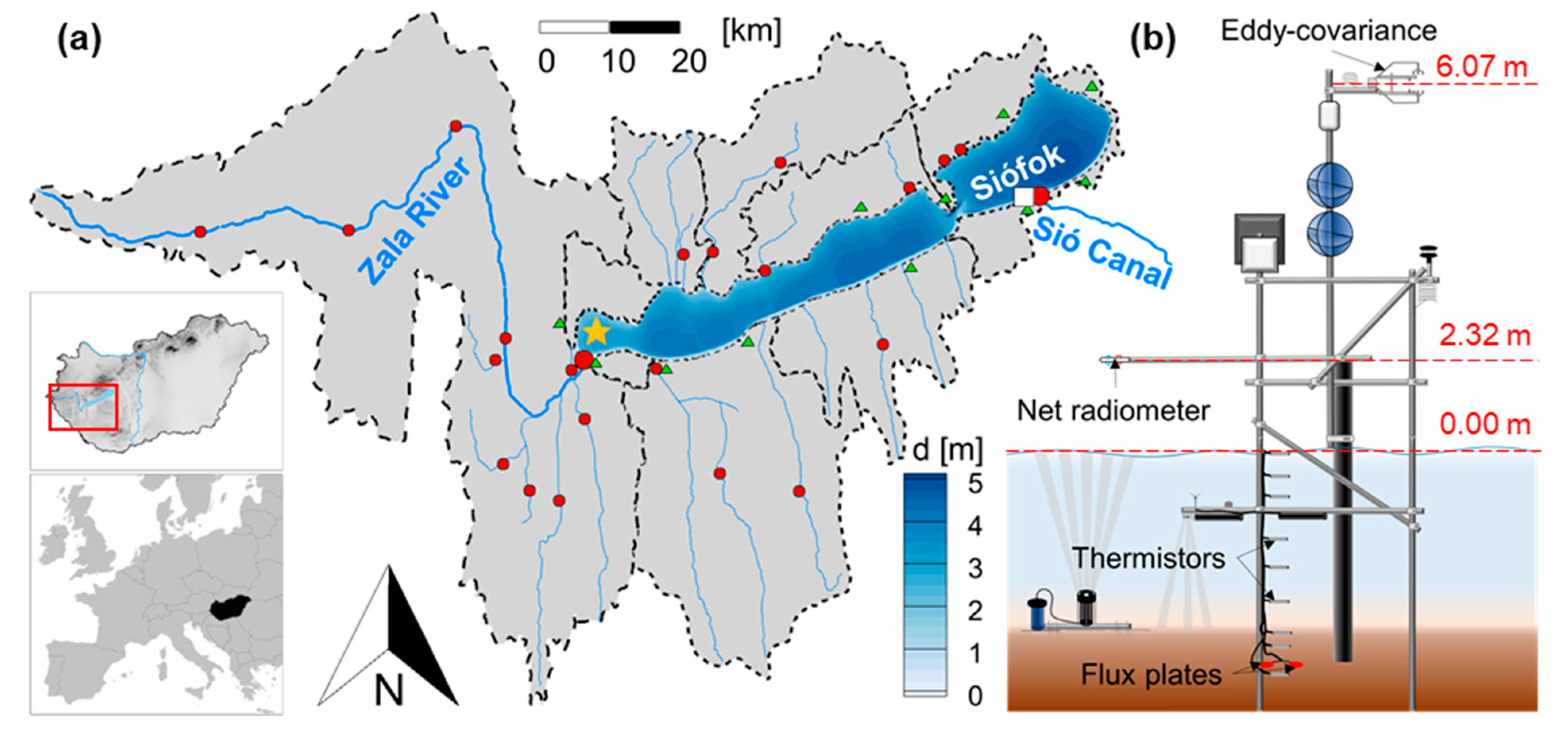
In our study, we use several measurements and evaporation estimation methods to reveal the variabilities mentioned above. Seasonal variations are explored by direct (EC) latent heat flux measurements and energy balance calculations. We invoke two well-accepted methods to corroborate our findings: the Priestly-Taylor and Penman-Monteith equations. Intra-annual evaporations are then determined by long-term (11 years) water balance analysis that provides monthly evaporations from which latent heat flux transfer coefficients can be derived using routine meteorological measurements. First, we present the study site (Lake Balaton, Transdanubian region, Hungary), second the EC measurements, and then the different methods with their input observational data sets.

2.1. Study Site

Lake Balaton is the largest freshwater lake in Central Europe. Its surface area is 596 km2, while its mean depth is only 3.2 m. The lake is situated in mid-latitudes characterized by a predominantly warm-summer humid continental climate. Due to the shallowness, it is a polymictic lake characterized by diurnal stratifications and mixings [22]. It has an elongated shape, and the main axis of the lake is nearly perpendicular to the most prevailing north-northwest (NNW) wind direction that results in strongly fetch limited conditions characterized by very young wave states. Over the water surface, the fetch is ~7 km on average in cases of NNW and (the second most frequent) southwest (SW) winds. The surface area variation as a function of water level is negligible because of the flat bathymetry and since two-thirds of the shoreline is built. Furthermore, the water level is regulated through a sluice gate at the outlet. As a result, the water level variation is also moderate (~40–50 cm).

2.2. The Eddy Covariance Measurements and the Monin-Obukhov Similarity Theory

Detailed hydrometeorological measurements were carried out in the middle of the westernmost basin of Lake Balaton between May 18th and October 4th in 2019 (with a measurement failure and lack of data between September 5th and 17th). The measurement aimed to have a detailed insight into the energy balance of the lake. The meteorological driving forces were completed with high-frequency flow, wave, and water level recordings. The characteristic fetch is ~2–10 km at the measurement station, although, in NNW, SW, and SE wind directions, it is about the same ~3–4 km. The station’s instrumentation can be seen in Figure 1b. An eddy-covariance setup operating at 10 Hz directly measured the water vapor heat flux. It consisted of a CSAT3 sonic anemometer and an EC150 open-path gas analyzer (Campbell Sci., Logan, CA, USA both). To reveal the EB, net radiation, water temperature profile, and heat exchange at the lakebed were also measured. The incoming and outgoing shortwave and longwave radiations were measured with a four-component CNR4 radiometer (Kipp and Zonen, Delft, The Netherlands). The water temperature profile was measured with a T107 thermistor chain (Campbell Sci., Logan, CA, USA) with 0.5 m vertical resolution. The top sensor was mounted on a buoy measuring a temperature at about 2 cm depth, while the other sensors were at fixed depths. The sediment heat flux was measured with heat flux plates (Hukseflux, Delft, The Netherlands) installed 10 cm deep in the sediment. At the observatory location, the water depth varied between 3–3.5 m, providing a good representation for the whole lake.
The raw eddy-covariance (EC) data was post-processed, and turbulent heat fluxes were calculated with the Turbulence Knight 3 (TK3) software (University of Bayreuth, Bayreuth, Germany) [23]. Post-processing included a double rotation, Moore [24], Webb [25], and Schotanus [26] corrections. The quality of fluxes was evaluated using Foken’s evaluation system, which aimed to determine turbulence stationarity conditions [27]. This method distinguishes 9 quality classes (1–best, 9–poor), and the data was accepted if it was classified as 7 or lower. The fluxes were determined as 20-min averages. Our earlier published work based on literature and sensitivity analysis detailed the data processing and the quality assurance/control filters [28]. There was 77.3% of the data in the first three quality classes, while 7.6% was rejected. As to the gap-filling, missing values were calculated using linear functions derived based on the accepted data points with a quality class equal or lower than 7. In the case of momentum, the friction velocity was calculated as a function of wind speed. Sensible and latent heat fluxes were calculated as a function of wind speed multiplied by temperature or specific humidity gradient, respectively. Missing values in routine meteorological data (wind speed, air temperature, humidity, water temperature) were scarce and covered short periods (few hours at most); thus, they were linearly interpolated.
Since the EC technique directly measures momentum and heat fluxes, it can be connected to the flux-gradient or the otherwise known Monin-Obukhov Similarity Theory (MOST). MOST assumes stability-dependent logarithmic wind, temperature, and humidity profiles above the surface to determine fluxes. The profile equations can be written as:
U z = u * κ ( ln ( z z 0 ) ψ m ( z L ) )
θ z θ 0 = θ * κ ( ln ( z z 0 H ) ψ H ( z L ) )
q z q 0 = q * κ ( ln ( z z 0 q ) ψ q ( z L ) )
where U is the wind speed, θ is the potential temperature, q is the specific humidity, z is the measurement height, z 0 , z 0 H and z 0 q are the roughness length for momentum, heat, and water vapor, respectively, ψ m , ψ H and ψ q are the universal stability functions for momentum, heat, and water vapor, respectively and L is the Obukhov length showing the atmospheric stability, κ is the von Kármán constant, u * is the wind friction velocity, T * is the temperature scale, q* is the humidity scale from which the turbulent fluxes can be expressed as:
τ = ρ a · u * 2  
H = ρ a · c p · u * · T *
L E = ρ a · λ · q * · u *
where τ is the wind stress (or momentum flux). In the absence of high-frequency observations but having gradient measurements, MOST can be simplified to the commonly applied bulk equations using transfer coefficients as follows [9]:
τ = ρ a · C D · U 2
H = ρ a · c p · C H · U · ( θ s θ a )
L E = ρ a · λ · C q · U · ( q s q a )
where CD is the drag coefficient, CH and Cq are the transfer coefficients for heat and water vapor, respectively, U is the wind speed and θ is the potential temperature. Water vapor transfer coefficients (Cq) were also calculated using the LEs obtained from the WB and based on the synoptic meteorological observations (wind speeds, temperatures, and humidity differences). Using the MOST and EC flux measurements, roughness lengths were derived by rearranging Equations (1)–(3). This required universal stability functions which were taken from the literature [29,30]. Transfer coefficients were calculated using EC data together with Equations (7)–(9). Both roughness lengths and transfer coefficients were evaluated as 20-min averages following the time resolution of EC fluxes.

2.3. Energy Balance Calculations

It has already been shown by several research groups that the EC technique cannot measure large-scale turbulent structures of the atmosphere, and the actual turbulent heat fluxes might be larger than the EC measured values [31,32,33]. As a result, the local EB cannot be closed, and a residual is formed. By neglecting the horizontal heat exchange, the EB of the water column per unit area can be written as:
H + L E = R n + Δ S + G + r e s
where H is the sensible heat flux, LE is the latent (or evaporative) heat flux, Rn is the net radiation, G is the heat exchange at water-sediment interface, ΔS is the energy storage change of the water body, and res is the residual. ΔS was determined from the depth-averaged water temperature change [34] which was derived using the measured vertical temperature profile, taking the depth variation into account. The energy budget closure (EBC) is the ratio of the two sides of the EB equation without the residual. A commonly used technique to solve the imbalance is that the residual is divided between the turbulent heat fluxes according to the Bowen ratio [3,4,6,7], which is expressed as [35]:
B o = H L E
To ensure the energy balance closure (EBC = 1), in our analysis, sensible and latent heat fluxes were recalculated and corrected. In this calculation, a sparser, daily time resolution was used in order to decrease the effects of the horizontal advective heat exchange.

2.4. Water Balance Method

On a monthly scale, lake evaporation can be determined by employing the water balance (WB) equation [21], from which evaporation (E) can be obtained as follows:
E = P + I Δ V W O
where Δ V is the change in the lake’s water volume, P is the precipitation, I = IZala + Istreams is the inflow from catchment runoff (IZala—inflow from Zala River, Istreams—inflow from further streams), W is the water usage, O is the outflow. However, the components on the right side of the equation were measured, their values may be subject to different types of errors, causing uncertainty in the estimated evaporation rate. To quantify it, we calculated the evaporation by a Monte-Carlo approach. We added an error term to each component on the right side of Equation (12). Based on the statistical analyses of the long-term WB components, we could assume that the error terms follow a normal distribution having two parameters: a mean and a standard deviation. The former one naturally equals zero. Following the comprehensive study of Winter [36], on a monthly scale, uncertainties are likely between 5–50% depending on the component. We assumed that the measured values might suffer from a maximum error of 50% based on the study. So, the two standard deviations (2σ) equaled 50% of the measured monthly values, respectively. One thousand error terms were randomly generated with normal distribution for each month and each component and added to the measured monthly values. This resulted in a set of evaporations for each month.
The Water Directorate has measured the monthly WB components of Lake Balaton since 1921 [37]. In this study, we used the WB data of the last 11 years, between 2010–2020. The precipitation falling over the lake was measured with 9 to 11 rain gauges depending on the year. The total precipitation was calculated using the Thiessen-polygon method. The inflow is the sum of measured discharges (Q) of the rivers and streams. Zala River has the largest sub-catchment and discharge (Q ~6–15 m3/s) and thus has the most detailed monitoring system. The incoming flow was measured by an acoustic flow sensor (Teledyne RDI Channel Master ADCP, Thousand Oaks, CA, USA). Small streams are monitored by automatic, telemetric water level gauges and occasional discharge measurements from which first rating curves and then discharge time series are evaluated. The runoff from ungauged catchments means a small proportion, and it is estimated from the precipitation falling over the catchment by employing monthly rainfall-runoff coefficients derived from regular system measurement campaigns. The water usage includes measured drinking, industrial, and agricultural water outtakes through monitored pumping stations. The only outflow of the lake is in Siófok and regulated by a monitored sluice gate. The water volume change is monitored by 8 water level gauges on the lake’s perimeter by 10-min resolution.
As an overview, Lake Balaton’s water balance components are shown in Table 1 for the EC measurement period in 2019. In Figure 2, we present the monthly means of each component based on the 11-year period from 2010 until 2020. It can be seen that in the case of Lake Balaton, the dominant water supplies are the inflow from the Zala River and the precipitation falling over the lake, while the most significant loss is arising from the evaporation since the water usage is low and the outflow is firmly restrained.
From the estimated evaporation, first, the monthly mean latent heat flux (LE) was calculated as follows:
L E = ρ w · λ · E Δ t
where ρ w is the density of water, λ is the latent heat of vaporization, and Δ t is the elapsed time (28–31 days) depending on the actual month. Second, the monthly transfer coefficient for LE was determined using Equation (9) from the Monte-Carlo simulation resulting set of evaporations. This required monthly mean wind, air temperature, and relative humidity measurements above the surface together with water surface temperature observations.
For the study period of 2010–2020, routine meteorological data were gathered from a synoptic station. It is located in Siófok, at the south shoreline, and operated by the Hungarian Meteorological Service (HMS) (Budapest, Hungary). This includes hourly data of wind speed, air temperature, relative humidity, and incoming solar (shortwave) radiation. The HMS also measures water temperature near the shoreline in 1 m depth at a location where the water depth varies between 2–2.5 m from which qs and θs (in Equation (9)) were determined. We could assume that the water temperature in 1 m depth is close to the surface value since the water column is usually well-mixed, and the vertical temperature profile becomes almost homogeneous at this location. This location is at the south shoreline, where the fetch is ~10–15 km in the case of the prevailing wind, which results in wave motions even for weak winds.

2.5. Penman-Monteith and Priestly-Taylor Methods

We have chosen two well-established evaporation estimation methods to (i) corroborate the EC and WB-based results considering seasonal variations and (ii) test their performance for subsequent climatic analysis when only routine hydrometeorological data are available. The Penman-Monteith (PM) and Priestly-Taylor (PT) methods calculate the latent heat flux based on fundamental physical principles combining energy and mass balances. The PM equation is written as:
L E = Δ · ( R n + Δ S + G ) + ρ a · c p · ( e s e a r a ) Δ + γ
where Δ is the slope of the saturation vapor pressure-temperature curve, e s is the saturation vapor pressure, e a is the actual vapor pressure, r a is the aerodynamic resistance, γ is the psychrometric constant. The resistance can be calculated as a function of wind speed and roughness lengths for momentum and vapor [35]. We applied the median values of the EC-derived roughness lengths.
The Priestly-Taylor (PT) method is the simplified version of the PM. The vapor deficit and convection terms are reduced to an empirical constant called the Priestley-Taylor coefficient (α). In this study, it was set to the widely accepted α = 1.26. Its value over water surfaces may vary between 1.1 and 1.4 [14,34,38], especially in a diurnal scale [11,39,40,41]; however, it was confirmed by many theoretical studies and observations that 1.26 is feasible in most of the cases [13,42]. The PT equation is written as:
L E = α ·   Δ · ( R n + Δ S + G ) Δ + γ
For the 2019 measurement period, Cq values were back-calculated using Equation (9) and the hydrometeorological measurements. The PT and PM methods can be used on a daily time scale, thus first, daily Cq values were derived from which monthly means, medians, minimums, maximums, 25th and 75th percentiles were determined.

3. Results

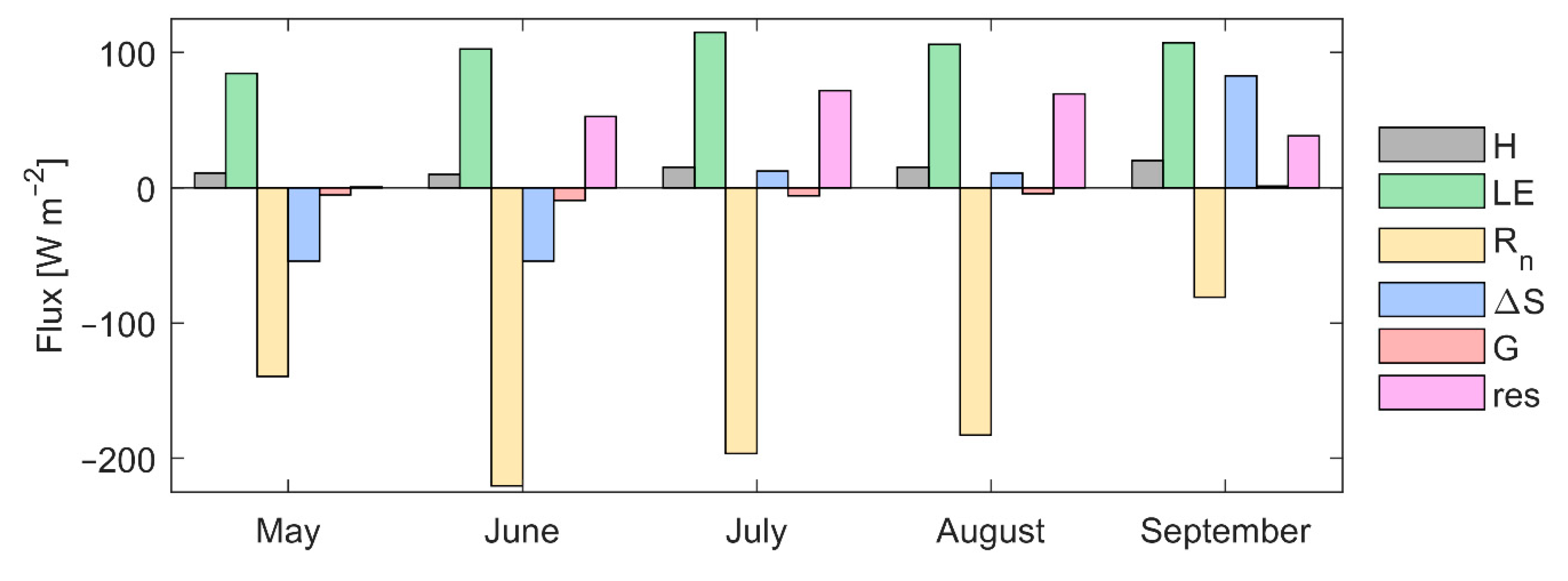
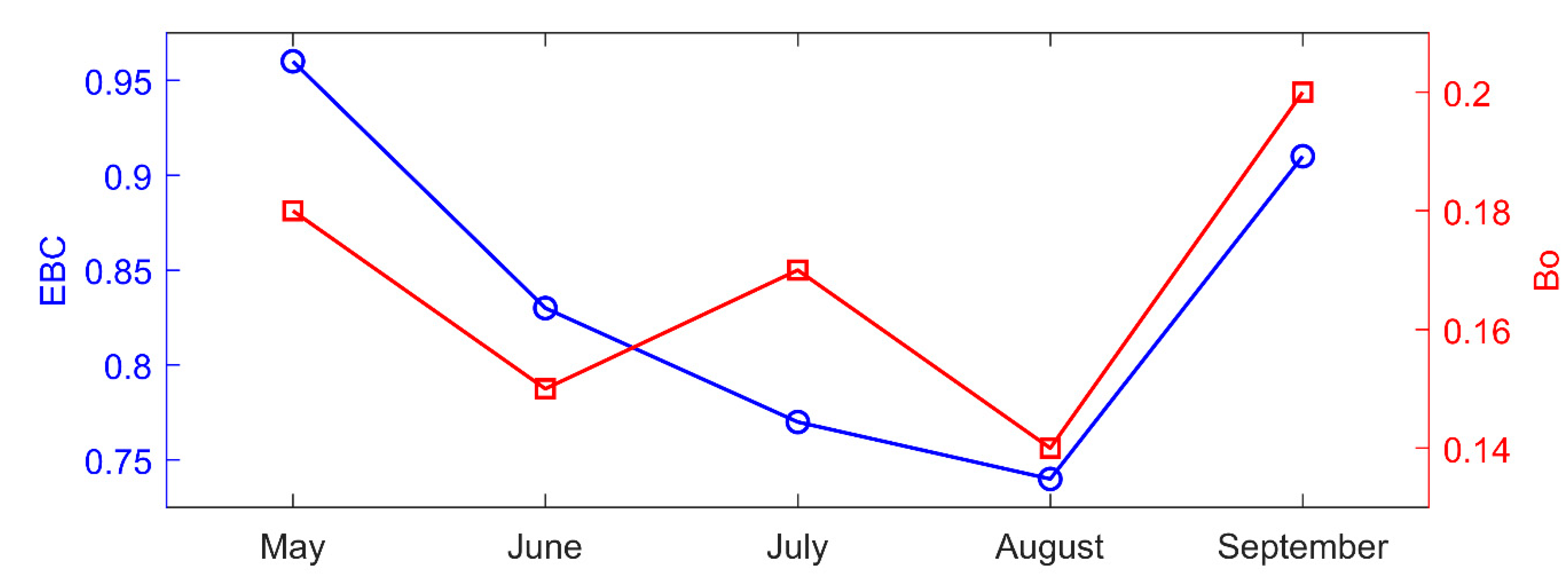
3.1. Energy Balance Characteristics of Lake Balaton

The EB of Lake Balaton was determined for five months in the warm season to analyze intra-seasonal variations. Complete months were June, July, and August, and the months not completely measured were May and September. The EB processes are typically characterized by strong diurnal cycles, especially the lake’s thermal structure. Due to the shallowness, weak thermal stratification (~1–5 °C surface-to-bottom difference) evolves during the daytime and breaks up at night. The earlier one is forced by the incoming solar radiation while the latter one is induced by the outgoing longwave radiation and turbulent heat fluxes which result in a strong surface cooling and an overturn. For a typical and indicative period, the energy budget components and the thermal structure of the lake are shown in Figure 3, together with the EBC ratios. The daily cycles of net radiation stored heat and sensible heat flux were apparent. In contrast, the evaporative heat flux typically did not have a daily cycle. The EB residual was usually positive and quite high (res ~100 W m−2 on average) and also had a mild diurnal cycle. The EBC ratio usually varied between ~0.4–0.9, and it was lower in the afternoons. A stronger stratification can be seen between 9 August and 13 August 2019, where the temperature difference between the surface (Ts) and the bottom (T350cm) reached Ts-T350cm ~4 °C (Figure 3c). When the wind was stronger between 13 August and 15 August, on the one hand, H and LE increased, while on the other hand, water temperature became homogeneous along with the depth, meaning vertically well-mixed conditions.
The monthly mean values of the EB components are provided in Figure 4. The stored energy was high in May and June ( Δ S > 50 W m−2), leading to a strong water temperature increase, with the energy primarily released back to the atmosphere only in September ( Δ S < −80 W m−2). The sediment heat flux (G) had similar intra-seasonal variation as H and LE, it was the highest in June (G > 9 W m−2). The ratio of G and H was ~0.4 on average, suggesting that thanks to the shallowness, G played a similar role as H in the EB of Lake Balaton.
The monthly averaged energy budget closure was between EBC ~0.74–0.97 and had a seasonal variation showing lower EBC values in July and August when water temperatures became closer to the equilibrium and changed considerably throughout the month (Figure 5). The Bowen ratio also showed a moderate intra-seasonal cycle varying between Bo ~0.14–0.20. The lowest Bo was observed in August and the higher ones in the warming and cooling periods, although it was higher in July than in June and August.

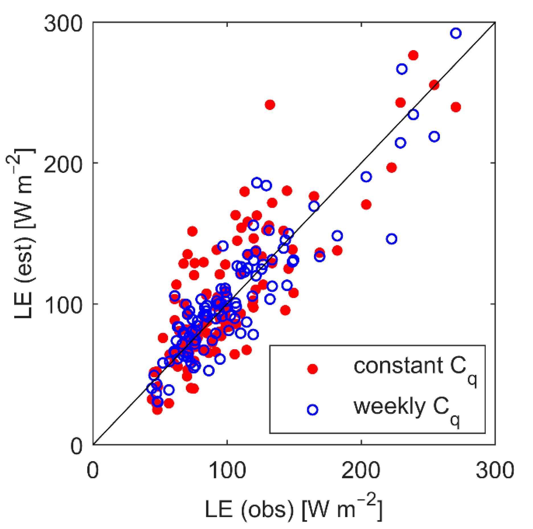
3.2. Comparison of Latent Heat Flux Estimations

To evaluate and corroborate EC-measured and WB-derived evaporations, monthly LEs were calculated with the three methods described above. First, EC-measured values were corrected according to Bo to ensure EB closure. Furthermore, LEs were determined employing the Penman-Monteith and Priestly-Taylor methods. Figure 6a shows the monthly values of LEs by employing all these methods. Monthly averaged LE fluxes varied between ~60–175 W m−2 during the analyzed period. The EC technique usually provided the lowest LEs of all, while the EB closure yielded the highest ones. WB resulting LEs were in the middle. All methods reproduced the intra-seasonal variation even the ones that didn’t rely on EC observations (Figure 6a). The evaporative fluxes with the different methods are compared to the EC measured values in Figure 6b. The EB-based PM and PT methods differed with ~23% to the EC-measured values on average, LEs were higher in the summer months and lower in the spring and fall months. The WB-based LEs were higher every month except in May (~23% difference on average). The highest difference was observed using the EB closure, with a correction of +39% on average compared to the EC data. Since the EB closure was always lower than EBC < 1, corrected values became higher in all months. The comparison of the EB closure-based values to the other methods suggested that the Bo ratio method (to distribute energy excess) might not be in every month valid and lead to an LE overestimation in May and August. This also means that the EC-measured Hs were more underestimated than LEs, as has been reported by several researchers in the case of land surfaces [43]. A combined method, when EB and WB closures are both fulfilled, can be suggested. In short, one can summarize that the intra-seasonal variation of evaporation was well represented by the EC measurement; however, it probably underestimated the monthly LEs.

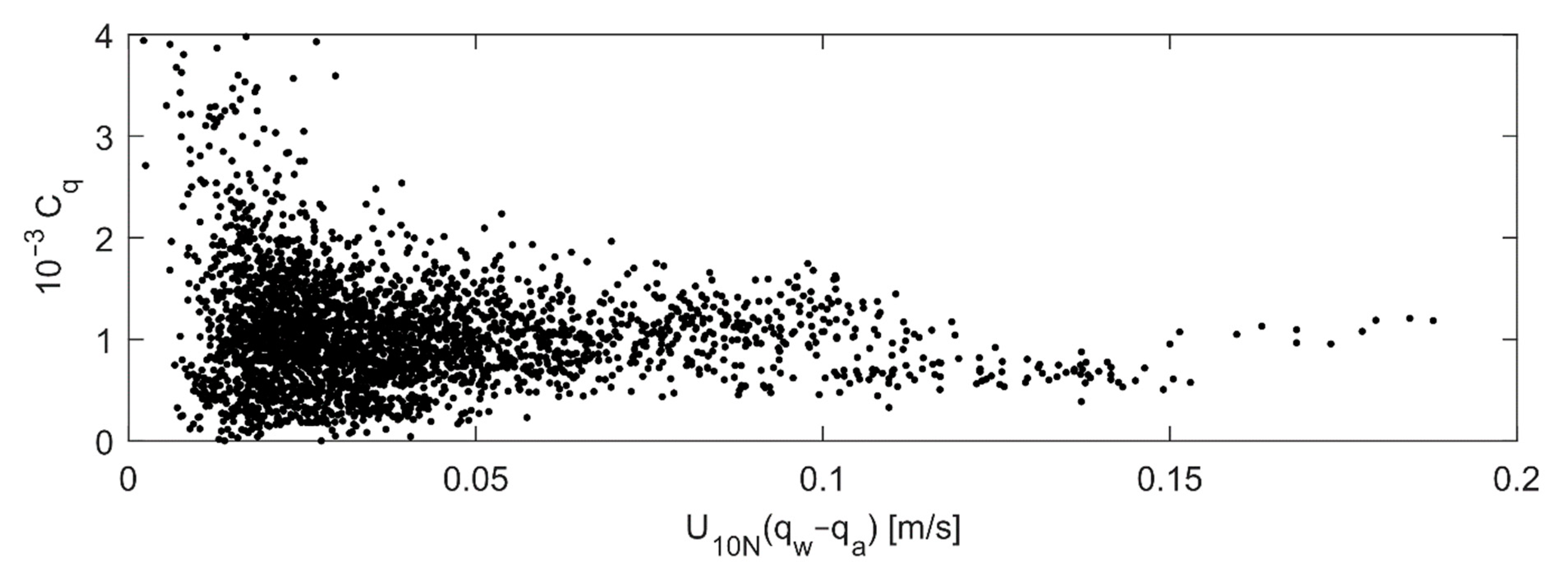
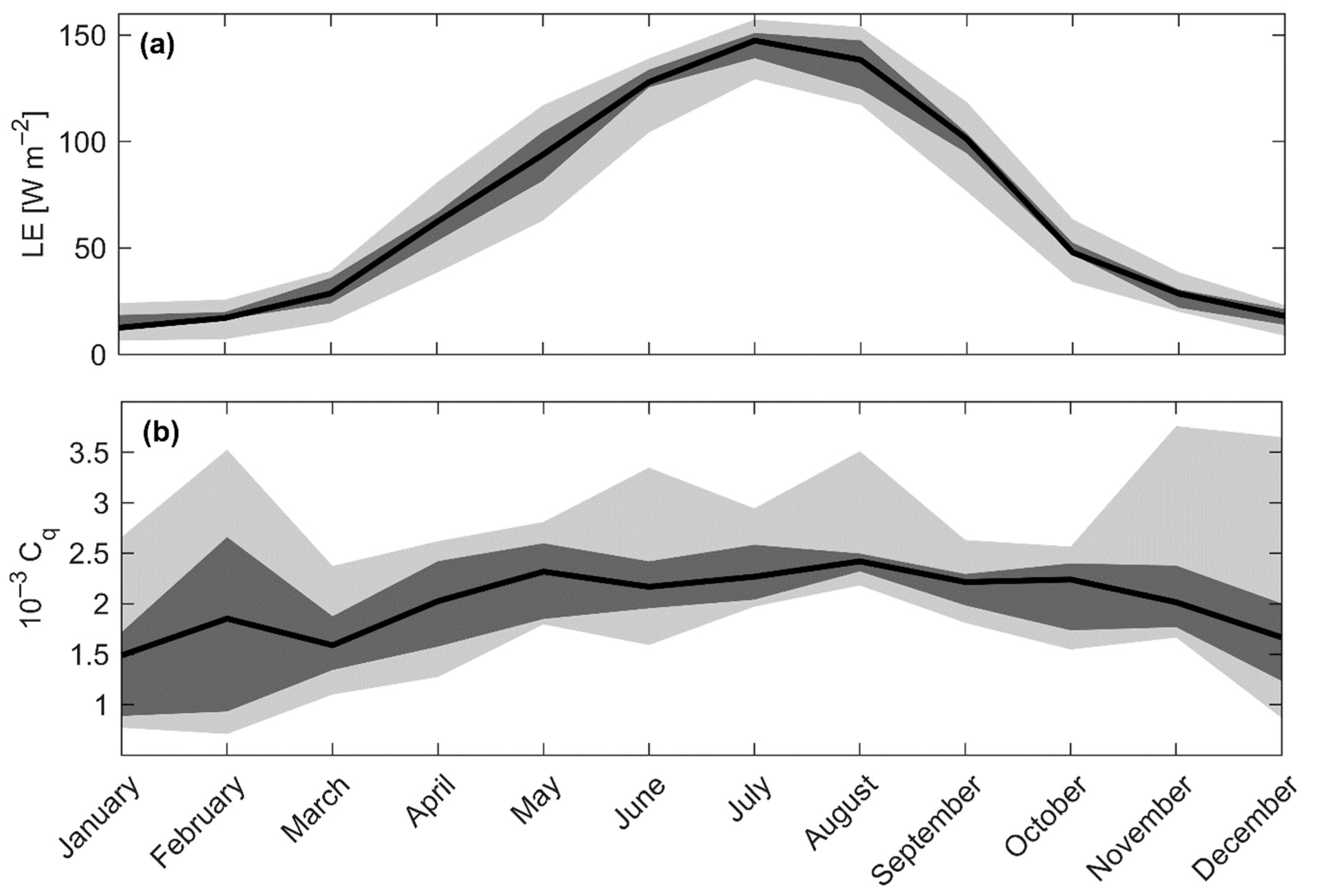
3.3. Seasonal Variability of the Water Vapor Transfer Coefficient

The transfer coefficient-based bulk equation (Equation (9)) is commonly used to calculate LE since it can provide estimates on a sub-daily scale. Cq is mostly approximated by a constant value or as a function of wind speed and humidity difference. In our case, Cq showed a somewhat weak relationship with the wind speed multiplied by the specific humidity difference based on EC data (Figure 7). Not shown here, but a similar finding was obtained for the sensible heat transfer coefficient (CH). Based on the dataset, a constant water vapor transfer coefficient should be suggested as Cq ~1.2 × 10⁻³.
As it was described in the Methods, we derived the monthly medians, minimums, maximums, 25th and 75th percentiles of Cq from the EC observations and also based on the LEs provided by the other methods using the observed surface temperature, humidity, and wind data (Figure 8). Although the monthly values of Cq varied somewhat depending on the method, the seasonal variation was apparent without exception. In general, Cqs obtained by the different methods were in good agreement. The only remarkable exception was the EB-based Cq in May when LE was also overestimated. The PM and PT results were very similar to each other and to the EC-measured values in spring and fall, but higher in summer months. The scatters of the PM and PT methods varied seasonally, but they were higher on average than the EC, EB, and WB methods. On average, the uncertainty was the lowest when employing the WB method except for May, where the other methods had a small scatter. Considering the 25th and 75th percentiles, Cq peaked in June for all methods except for WB; however, the median of the EB-based Cq was also lower in June than July. Based on these results, we could conclude that: (i) in the case of Lake Balaton, Cq shouldn’t be considered as a constant, and (ii) an intra-annual variation may exist.

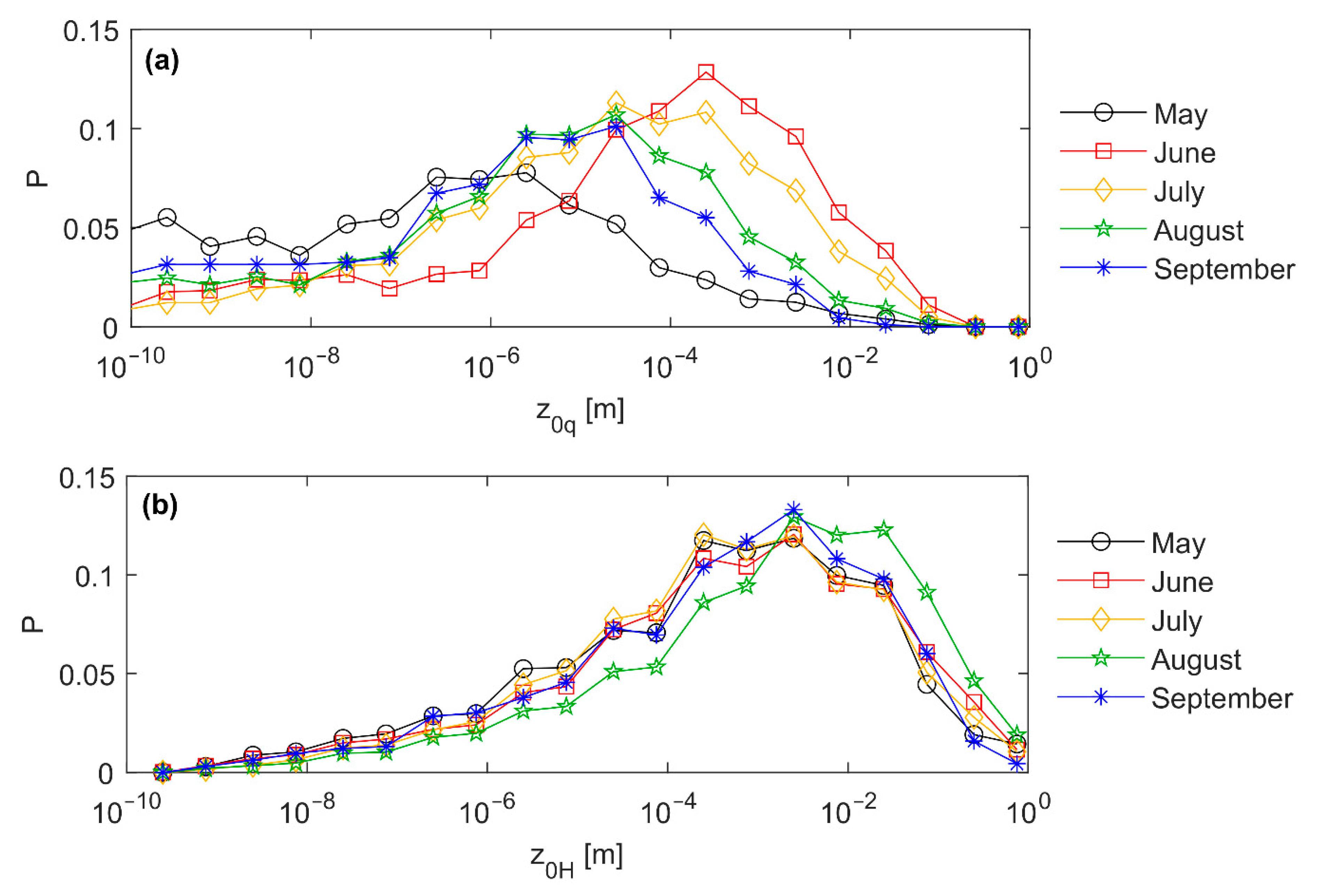
3.4. Seasonal Variability of Roughness Lengths for Water Vapor and Heat

Since Cq values showed a strong intra-seasonal cycle, roughness lengths were determined on a 20-min scale following the time resolution of EC-based fluxes. The probability density functions (PDF) of water vapor roughness length for each month can be seen in Figure 9a. Both median and peak values of the PDFs showed a clear seasonal cycle. The roughness length was the lowest in May (z0q ~10−6 m) and the highest in June (z0q ~5∙10−4 m) and it was continuously getting lower from July to September (from z0q ~10−4 m to z0q ~10−5 m). As to our knowledge, this type of seasonal variation of water vapor roughness length over lake surfaces has not been reported yet. In contrast, z0H, the roughness length for H, did not possess an intra-seasonal variation (Figure 9b), similarly to e.g., Wang et al. [44]. In the literature, both z0H and z0q are characterized with constant values or as a function of wind or stability-related parameters [35]. In short, z0H can be approximated with a median (z0H = 1.2∙10−3 m) or a peak value (z0H = 2.5∙10−3 m) while a constant value is clearly not able to represent z0q for the whole summer in the case of Lake Balaton and explains the monthly variation of Cq.

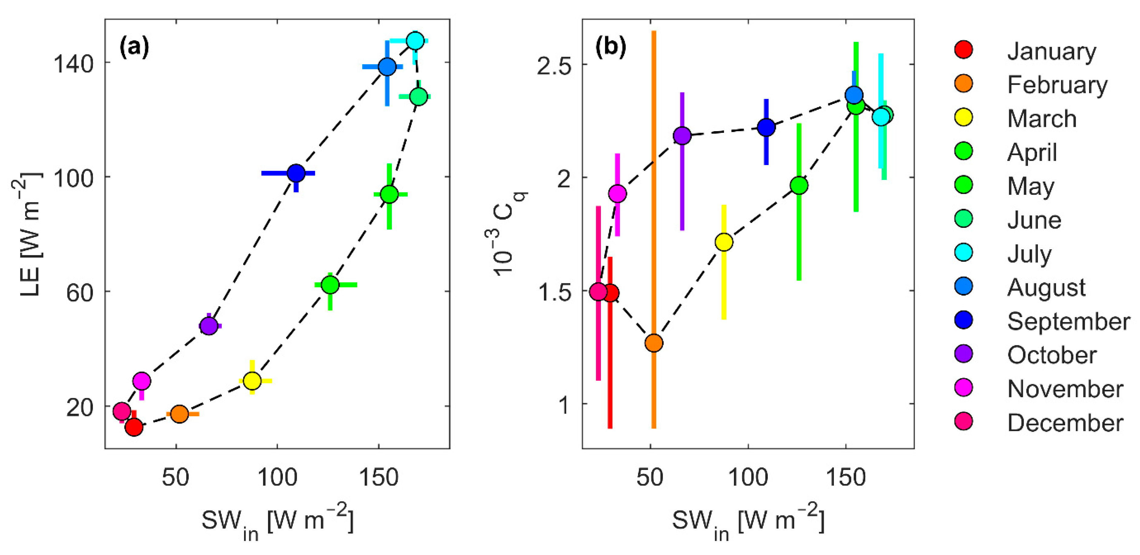
3.5. Drivers of Latent Heat Flux and Its Transfer Coefficient

The main drivers of evaporation have been explored on different time scales, from 20-min to 1-month. The determination coefficients (R2) were calculated to reveal the relationship between LE and its drivers [45,46]. The analyzed drivers consisted of routine hydrometeorological variables as wind speed (U), water surface temperature (Ts), temperature difference (ΔT = TsTa), specific humidity difference (Δq = qsqa), and atmospheric stability (z/L), and also of energy budget components, as Rn, ΔS, H, and res. The results of this analysis are presented in Figure 10a showing R2 by coloring. It can be seen that the U showed a high correlation (R2 ~ 0.7–0.8) with LE on time scales from 20-min to 1-week and became lower for longer time scales. ΔT showed a modest correlation (R2 ~0.5) at longer time scales from 1-week to monthly. Interestingly, the influence of Δq was quite low at all time scales, except at the monthly scale. This suggests that over the 3–4 km fetch, the saturation of air was low and could not be considered as a limiting factor. Furthermore, it is important to see that the involvement of Δq may not result in a better LE estimation since R2 values are lower in the case of U·Δq than in the case of U, even at the 20-min time scale. In short, we can conclude that for the fetch-limited Lake Balaton, wind dominates short time scales, while in the case of Δq, became more influencing only at the monthly scale. Considering the monthly scale, we also would like to highlight that the impact of water-to-air surface temperature difference (ΔT) is larger than Δq. There was a moderate correlation (R2 ~0.5) at a monthly time scale with the atmospheric stability. ΔS had an influence (R2 ~0.5–0.7) at time scales longer than daily. The relationship with H was always above R2 ~0.5 and reached R2 ~0.7 on a weekly time scale. A relationship was also revealed between the energy budget residual and LE on 2-week and monthly scales. Based on the correlation analysis, surprisingly no relationship was found between LE and Rn. Its cause and reliability are discussed in Section 4.2.
The same analysis was performed for the water vapor transfer coefficient (Figure 10b). At daily or shorter time scales, the correlation was very low with any of the analyzed hydrometeorological variables and energy budget components. In contrast, Ts correlated (R2 ~0.6) with Cq at weakly and longer time scales. On a monthly scale, we found moderate correlations (R2 ~0.5) with U·ΔT and U·Δq, as well as with ΔS and H. In opposition to the LE results, Rn showed a strong relationship with Cq on 1-week, 2-week, and monthly scales, having determination coefficients of R2 = 0.59, 0.85, and 0.93, respectively. Based on these results, the observed intra-seasonal variation of the water vapor transfer coefficient was possibly driven by the seasonally varying net radiation. This suggests that a constant Cq throughout the year should not be applied, but its value can be related to net radiation (see Section 4.2 for further details).

3.6. Intra-Annual Variation of the Water Vapor Transfer Coefficient

Using the available 11-year-long monthly water balance data of Lake Balaton, monthly LEs and the intra-annual variation of Cq were determined for whole years (Figure 11). First, as it was described in the Methods section, the WB equation provided monthly evaporations from which LEs were calculated. Second, using the synoptic hourly hydrometeorological data from Siófok, water vapor transfer coefficients were back-calculated. Monthly LEs did not possess as much scatter among years as Cq. Both LE and Cq are shown using 10th–90th and 25th–75th percentiles with light and dark grey shadings, respectively, and medians with black lines (Figure 11). The evaporation was the lowest in the winter with LE ~20 W m−2, while it usually reached its maximum in July or August, having LE over ~150 W m−2. Agreeing with our earlier presented results on the intra-seasonal variation of Cq, the long-time data series showed similar periodic behavior. The intra-annual variation was apparent, transfer coefficients were lower in the winter and higher in the summer months with a minimum of Cq ~1 × 10⁻³ and a maximum of Cq ~2.5 × 10⁻³, respectively, according to the 25th–75th percentile ranges. Comparing the decadal medians with the EC observations from 2019, some deviances can be captured. In 2019, Cq peaked in June (based on EC measurement) or July (based on the other methods), while based on the long-term WB data, it mostly peaks in August; however, Cq possesses a high variability both in June and August. In summary, the long-term WB-based analysis has confirmed the intra-seasonal Cq variation that resulted from the EC measurements and furthermore, it has revealed its notable annual cycle.

4. Discussion

4.1. Latent Heat Flux Estimation Using Time-Varying Transfer Coefficients

Both measurements and estimations have revealed an apparent and intra-seasonal variation of Cq. According to the correlation analysis, its value was driven by Rn on a 1-week time scale. In order to show the benefit of using time-varying Cq in the estimation, we calculated daily LEs both with constant and time-varying coefficients and compared them to the EC results (Figure 12). Cq = 1.2 × 10⁻³ was applied as the constant, while for the latter case weekly Cq averages were derived. The determination coefficient R2 increased from 0.52 to 0.84 proving the validity of the time variable coefficient. The root mean square errors reduced from 34.4 to 20.1 W m−2 for constant and weekly varying transfer coefficients, respectively, while the mean bias improved to 0.19 from 5.44 W m−2. This clearly showed that we can increase the accuracy of bulk formulations which serve several aims, such as boundary conditions in the lake and meteorological models as they are commonly used with sub-daily time resolution. Furthermore, simple bulk formulations are also frequently applied to determine lake evaporations on a monthly scale [13,34]. In conclusion, it would be advantageous to apply intra-seasonally varying water vapor transfer coefficients for evaporation estimation; however, to reveal the intra-annual variation, EC, EB, or WB measurements should last for at least one year.

4.2. Hysteresis Behavior of Evaporation and Its Transfer Coefficient to Radiative Heat Flux

A surprisingly weak relationship has been found between Rn and LE using the EC and in-situ hydrometeorological observations; however, it was reported by many studies that the radiative heat flux plays a dominant role in evaporation on a monthly scale [14,45]. The weak correlation can be attributed to the hysteresis behavior between incoming radiation and LE [47]. Since Rn data were not available for further months, we used the incoming shortwave radiation (SWin) instead which is the dominant term in the net radiation and available for several decades from the synoptic meteorological station. In Figure 13a, we plotted the monthly course of LE (obtained by the WB calculations) and measured SWin. A clear hysteresis behavior can be revealed: in the warming period (January–July), the relationship between LE and SWin can be approximated with exponential, while in the cooling period (July–January) with a linear function. The EC measurement period (May-September) was around the turning point in July that led to the weak correlation. Nevertheless, a clear and strong relationship can be established between the two variables for the shallow Lake Balaton similar to other lake studies [14,46,48]. In other words, the available energy (which is driven by SWin) plays a crucial role in the intra-annual variability of LE.
Since a strong correlation has been observed between Cq and Rn (Figure 10b), the monthly courses were determined for Cq and SWin (Figure 13b). A clear hysteresis behavior existed between these two variables as well; however, in this case, the hysteresis curve showed a more complex shape. The loop’s area was significantly smaller between May and August and Cq values had lower scatter that might lead to the high correlation values between Cq and Rn in Section 3.5. In contrast, in the cool period (September-April), the loop opened wide and the variability of Cq significantly increased. Nevertheless, these findings have corroborated again the intra-annual variability of Cq and the validity of seasonally varying transfer coefficients.

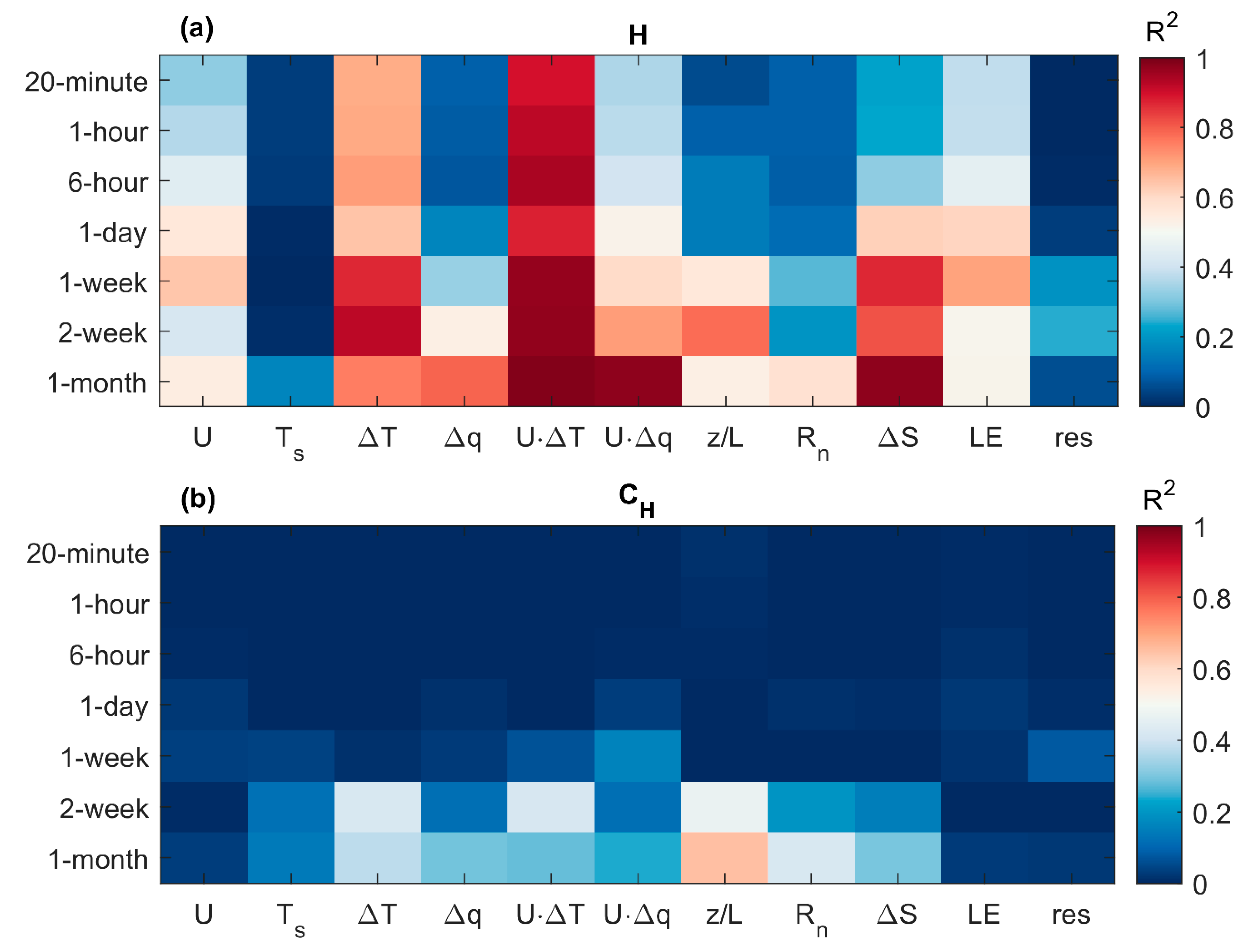
4.3. Drivers of Sensible Heat Flux and Its Transfer Coefficient

Besides LE, the same correlation analysis of forcing factors was carried out for H (Figure 14a) and its transfer coefficient CH (Figure 14b). The wind speed (U) had a moderate correlation (R2 ~0.5–0.6) at all of the time scales with H, especially in weekly or longer scales. Ts didn’t show a remarkable relationship with H, in contrast to ΔT which provided high correlations (highest at 1-week and 2-week scales). If U was multiplied by ΔT, the determination coefficient became very high (R2 > 0.85) at every time scale. On 2-week and monthly scales, the correlation was also high with Δq and also if it was multiplied by U. The atmospheric stability (z/L) also had a moderate correlation at longer time scales with H. In contrast to LE, ΔS showed a strong relationship with H, having an increase by the time scale.
Considering CH, it did not have remarkable correlations with any variables as we expected since neither EC-derived z0H nor CH showed an intra-seasonal variation. A notable correlation was only obtained with z/L on monthly and weekly scales, while some weak correlation could be seen on longer time scales with ΔT, Δq, U, and also with Rn and ΔS (Figure 14b). In short, this simple analysis underpinned that H is primarily forced by the ΔT and U, while CH can be handled as a constant along the year without invoking any other EB terms or auxiliary hydrometeorological data.

5. Conclusions

A five-month-long eddy-covariance measurement has been carried out in Lake Balaton to accurately measure evaporation of a large but shallow freshwater lake in the mid-latitudes. The EC measured evaporation and water vapor transfer coefficients have been compared to the results of energy balance and water balance methods on a monthly scale. Turbulent fluxes were significantly underestimated (~16% on average) with the EC method compared to the other ones. Having seen the results of the other techniques, we have concluded that the energy residual distribution by the Bowen ratio is not always applicable. We came to this conclusion since the EB-based evaporation estimates were remarkably higher in May and in August than the other estimates by closing the energy imbalance employing the Bowen ratio. These are the warming and cooling periods. This means that a higher portion of the energy residual belongs to the sensible heat flux than as it comes from the Bowen ratio. In other words, sensible and latent heat fluxes are underestimated with different degrees during these periods.
The EC-derived monthly z0q distributions showed an apparent intra-seasonal variation which was not reported yet as to our knowledge. Consequently, the EC-derived Cqs possessed the same variability. The partly energy balance-based Penman-Monteith and Priestley-Taylor, as well as the WB-based methods, gave nearly identical results and corroborated this finding. Considering the two former methods, we found that they can provide realistic evaporation estimations for the shallow Lake Balaton, but only if the heat storage term was included in the calculation. On average, the four methods (EB, WB, PT, and PM) resulted in very similar monthly Cq values. EC-derived values were mostly lower suggesting again that the EC technique might underestimate lake-wide evaporation rates. The primary drivers of LE and Cq vary at different time scales. Nevertheless, the main driving hydrometeorological variables are the wind speed, the specific humidity difference in the case of LE, and the net radiation for Cq. The latter relationship can be characterized by hysteresis.
The most important result is that LE estimation is more accurate if we apply an intra-seasonally varying Cq rather than a constant, which is generally used in the literature for lake evaporation. The observed intra-seasonal Cq variation agrees well with its intra-annual behavior estimated using the long-term WB data. Cq is larger in the summer months (June, July, and August) than in the winter ones (December, January, and February), having a median value of 2.3 × 10⁻³ and 1.7 × 10⁻³, respectively. The median value on an annual scale is 2.0 × 10⁻³. This finding has an outcome for lake and meteorological model applications. Transfer coefficient-based bulk equations are commonly applied as parametrizations to quantify heat exchanges at the air-water interface. A time-independent average value would result in over- and underestimation of LEs depending on the season that might be handled by a false calibration of other model parameters to obtain good agreement between observations and model results. The intra-annual variation of Cq in Lake Balaton suggests performing similar analyses for other lakes to reveal the situation when this variability has to be considered. Finally, the intra-annual behavior of Priestley-Taylor’s α should also be considered for a similar investigation.

Author Contributions

Conceptualization, G.L. and P.T.; methodology, G.L. and P.T.; formal analysis, G.L, P.T., and T.W.; investigation, G.L. and P.T.; resources, G.L., P.T. and T.W.; data curation, G.L.; writing—original draft preparation, G.L. and P.T.; writing—review and editing, G.L., P.T. and T.W.; visualization, G.L.; supervision, P.T. and T.W.; funding acquisition, P.T. and T.W. All authors have read and agreed to the published version of the manuscript.

Funding

The measurement campaign was performed in the frame of GINOP2.3.2-15-2016-00007, GINOP-2.3.2-15-2016-00055, OTKA-138176, OTKA-120551 (Interaction of physical processes across spatial and temporal scales in shallow lakes) and OTKA-134559 (Causes and consequences of the record-setting algal bloom in 2019: climate sensitivity of Lake Balaton) projects. This work has been supported by the ÚNKP-20-3 New National Excellence Program of the Ministry for Innovation and Technology (Budapest, Hungary). Through the first and second authors, the research was also supported by the FIKP grant of EMMI in the frame of the Water Sciences and Disaster Prevention research area of BME (BME FIKP-VIZ).

Institutional Review Board Statement

Not applicable.

Informed Consent Statement

Not applicable.

Data Availability Statement

The eddy-covariance and hydrometeorological observations, as well as the monthly water balance data are available from the authors upon request.

Acknowledgments

The authors would like to thank to the Hungarian Meteorological Service (Budapest, Hungary) and the Central-Transdanubian Water Directorate (Székesfehérvár, Hungary) to provide the required hydrometeorological and water balance time series.

Conflicts of Interest

The authors declare no conflict of interest.

References

  1. Lenters, J.D.; Cutrell, G.J.; Istanbulluoglu, E.; Scott, D.T.; Herrman, K.S.; Irmak, A.; Eisenhauer, D.E. Seasonal energy and water balance of a Phragmites australis-dominated wetland in the Republican River basin of south-central Nebraska (USA). J. Hydrol. 2011, 408, 19–34. [Google Scholar] [CrossRef] [Green Version]
  2. Xing, Z.; Fong, D.A.; Tan, K.M.; Lo, E.Y.M.; Monismith, S.G. Water and heat budgets of a shallow tropical reservoir. Water Resour. Res. 2012, 48. [Google Scholar] [CrossRef] [Green Version]
  3. Lenters, J.D.; Kratz, T.K.; Bowser, C.J. Effects of climate variability on lake evaporation: Results from a long-term energy budget study of Sparkling Lake, northern Wisconsin (USA). J. Hydrol. 2005, 308, 168–195. [Google Scholar] [CrossRef]
  4. Nordbo, A.; Launiainen, S.; Mammarella, I.; Leppäranta, M.; Huotari, J.; Ojala, A.; Vesala, T. Long-term energy flux measurements and energy balance over a small boreal lake using eddy covariance technique. J. Geophys. Res. Atmos. 2011, 116. [Google Scholar] [CrossRef]
  5. Li, Z.; Lyu, S.; Zhao, L.; Wen, L.; Ao, Y.; Wang, S. Turbulent transfer coefficient and roughness length in a high-altitude lake, Tibetan Plateau. Theor. Appl. Climatol. 2016, 124, 723–735. [Google Scholar] [CrossRef]
  6. Riveros-Iregui, D.A.; Lenters, J.D.; Peake, C.S.; Ong, J.B.; Healey, N.C.; Zlotnik, V.A. Evaporation from a shallow, saline lake in the Nebraska Sandhills: Energy balance drivers of seasonal and interannual variability. J. Hydrol. 2017, 553, 172–187. [Google Scholar] [CrossRef] [Green Version]
  7. Wang, B.; Ma, Y.; Ma, W.; Su, Z. Physical controls on half-hourly, daily, and monthly turbulent flux and energy budget over a high-altitude small lake on the Tibetan Plateau. J. Geophys. Res. 2017, 122, 2289–2303. [Google Scholar] [CrossRef]
  8. Yusup, Y.; Liu, H. Effects of atmospheric surface layer stability on turbulent fluxes of heat and water vapor across the water-atmosphere interface. J. Hydrometeorol. 2016, 17, 2835–2851. [Google Scholar] [CrossRef]
  9. Wang, B.; Ma, Y.; Chen, X.; Ma, W.; Su, Z.; Menenti, M. Observation and simulation of lake-air heat and water transfer processes in a high-altitude shallow lake on the Tibetan plateau. J. Geophys. Res. 2015, 120, 12327–12344. [Google Scholar] [CrossRef] [Green Version]
  10. Xiao, W.; Liu, S.; Wang, W.; Yang, D.; Xu, J.; Cao, C.; Li, H.; Lee, X. Transfer Coefficients of Momentum, Heat and Water Vapour in the Atmospheric Surface Layer of a Large Freshwater Lake. Boundary-Layer Meteorol. 2013, 148, 479–494. [Google Scholar] [CrossRef]
  11. Assouline, S.; Tyler, S.W.; Tanny, J.; Cohen, S.; Bou-Zeid, E.; Parlange, M.B.; Katul, G.G. Evaporation from three water bodies of different sizes and climates: Measurements and scaling analysis. Adv. Water Resour. 2008, 31, 160–172. [Google Scholar] [CrossRef]
  12. Choi, T.; Hong, J.; Kim, J.; Lee, H.; Asanuma, J.; Ishikawa, H.; Tsukamoto, O.; Zhiqui, G.; Ma, Y.; Ueno, K.; et al. Turbulent exchange of heat, water vapor, and momentum over a Tibetan prairie by eddy covariance and flux variance measurements. J. Geophys. Res. D Atmos. 2004, 109. [Google Scholar] [CrossRef]
  13. Metzger, J.; Nied, M.; Corsmeier, U.; Kleffmann, J.; Kottmeier, C. Dead Sea evaporation by eddy covariance measurements vs. aerodynamic, energy budget, Priestley-Taylor, and Penman estimates. Hydrol. Earth Syst. Sci. 2018, 22, 1135–1155. [Google Scholar] [CrossRef] [Green Version]
  14. Xiao, W.; Zhang, Z.; Wang, W.; Zhang, M.; Liu, Q.; Hu, Y.; Huang, W.; Liu, S.; Lee, X. Radiation Controls the Interannual Variability of Evaporation of a Subtropical Lake. J. Geophys. Res. Atmos. 2020, 125. [Google Scholar] [CrossRef]
  15. Zhao, D.; Li, M. Dependence of wind stress across an air–sea interface on wave states. J. Oceanogr. 2019, 75, 207–223. [Google Scholar] [CrossRef]
  16. Blanken, P.D.; Spence, C.; Hedstrom, N.; Lenters, J.D. Evaporation from Lake Superior: 1. Physical controls and processes. J. Great Lakes Res. 2011, 37, 707–716. [Google Scholar] [CrossRef]
  17. Subin, Z.M.; Riley, W.J.; Mironov, D. An improved lake model for climate simulations: Model structure, evaluation, and sensitivity analyses in CESM1. J. Adv. Model. Earth Syst. 2012, 4. [Google Scholar] [CrossRef]
  18. Heikinheimo, M.; Kangas, M.; Tourula, T.; Venäläinen, A.; Tattari, S. Momentum and heat fluxes over lakes Tamnaren and Raksjo determined by the bulk-aerodynamic and eddy-correlation methods. Agric. For. Meteorol. 1999, 98–99, 521–534. [Google Scholar] [CrossRef]
  19. Zou, Z.; Zhao, D.; Liu, B.; Zhang, J.A.; Huang, J. Observation-based parameterization of air-sea fluxes in terms of wind speed and atmospheric stability under low-to-moderate wind conditions. J. Geophys. Res. Ocean. 2017, 122, 4123–4142. [Google Scholar] [CrossRef]
  20. McGloin, R.; McGowan, H.; McJannet, D.; Burn, S. Modelling sub-daily latent heat fluxes from a small reservoir. J. Hydrol. 2014, 519, 2301–2311. [Google Scholar] [CrossRef] [Green Version]
  21. Honti, M.; Somlyódy, L. Stochastic water balance simulation for Lake Balaton (Hungary) under climatic pressure. Water Sci. Technol. 2009, 59, 453–459. [Google Scholar] [CrossRef] [PubMed]
  22. Torma, P.; Krámer, T. Modeling the effect of waves on the diurnal temperature stratification of a shallow lake. Period. Polytech. Civ. Eng. 2017, 61, 165–175. [Google Scholar] [CrossRef] [Green Version]
  23. Mauder, M.; Foken, T. Documentation and Instruction Manual of the Eddy-Covariance Software Package TK3. Arbeitsergebnisse 2011, 3, 60. [Google Scholar] [CrossRef]
  24. Moore, C.J. Frequency response corrections for eddy correlation systems. Boundary-Layer Meteorol. 1986, 37, 17–35. [Google Scholar] [CrossRef]
  25. Webb, E.K.; Pearman, G.I.; Leuning, R. Correction of flux measurements for density effects due to heat and water vapour transfer. Q. J. R. Meteorol. Soc. 1980, 106, 85–100. [Google Scholar] [CrossRef]
  26. Schotanus, P.; Nieuwstadt, F.T.M.; De Bruin, H.A.R. Temperature measurement with a sonic anemometer and its application to heat and moisture fluxes. Bound.-Layer Meteorol. 1983, 26, 81–93. [Google Scholar] [CrossRef]
  27. Foken, T.; Gockede, M.; Mauder, M.; Mahrt, L.; Amiro, B.; Munger, W. Handbook of Micrometeorology: A Guide for Surface Flux Measurement and Analysis: Chapter 9: Post-Field Data Quality Control; Springer: Dordrecht, The Netherlands, 2004; ISBN 978-1-4020-2264-7. [Google Scholar]
  28. Lükő, G.; Torma, P.; Krámer, T.; Weidinger, T.; Vecenaj, Z.; Grisogono, B. Observation of wave-driven air–water turbulent momentum exchange in a large but fetch-limited shallow lake. Adv. Sci. Res. 2020, 17, 175–182. [Google Scholar] [CrossRef]
  29. Dyer, A.J. A review of flux-profile relationships. Bound.-Layer Meteorol. 1974, 7, 363–372. [Google Scholar] [CrossRef]
  30. Shabani, B.; Nielsen, P.; Baldock, T. Direct measurements of wind stress over the surf zone. J. Geophys. Res. Ocean 2014, 119, 2949–2973. [Google Scholar] [CrossRef] [Green Version]
  31. Mauder, M.; Oncley, S.P.; Vogt, R.; Weidinger, T.; Ribeiro, L.; Bernhofer, C.; Foken, T.; Kohsiek, W.; Bruin, H.A.R.; Liu, H. The energy balance experiment EBEX-2000. Part II: Intercomparison of eddy-covariance sensors and post-field data processing methods. Bound.-Layer Meteorol. 2007, 123, 29–54. [Google Scholar] [CrossRef]
  32. Kanda, M.; Inagaki, A.; Letzel, M.O.; Raasch, S.; Watanabe, T. Les study of the energy imbalance problem with eddy covariance fluxes. Bound.-Layer Meteorol. 2004, 110, 381–404. [Google Scholar] [CrossRef]
  33. Foken, T. Micrometerology; Springer Science & Business Media: Berlin/Heidelberg, Germany, 2008; ISBN 9783540746652. [Google Scholar]
  34. Wang, W.; Xiao, W.; Cao, C.; Gao, Z.; Hu, Z.; Liu, S.; Shen, S.; Wang, L.; Xiao, Q.; Xu, J.; et al. Temporal and spatial variations in radiation and energy balance across a large freshwater lake in China. J. Hydrol. 2014, 511, 811–824. [Google Scholar] [CrossRef]
  35. Brutsaert, W. Evaporation into the Atmosphere; Springer Netherlands: Dordrecht, The Netherlands, 1982; ISBN 978-90-481-8365-4. [Google Scholar]
  36. Winter, T.C. Uncertainties in Estimating the Water Balance of Lakes. JAWRA J. Am. Water Resour. Assoc. 1981, 17, 82–115. [Google Scholar] [CrossRef]
  37. Central-Transdanubian Water Directorate. Determination of Lake Balaton’s monthly Water Balance Components for 2019; Central-Transdanubian Water Directorate: Székesfehérvár, Hungary, 2019. [Google Scholar]
  38. Dos Reis, R.J.; Dias, N.L. Multi-season lake evaporation: Energy-budget estimates and CRLE model assessment with limited meteorological observations. J. Hydrol. 1998, 208, 135–147. [Google Scholar] [CrossRef]
  39. Assouline, S.; Li, D.; Tyler, S.; Tanny, J.; Cohen, S.; Bou-Zeid, E.; Parlange, M.; Katul, G.G. On the variability of the Priestley-Taylor coefficient over water bodies. Water Resour. Res. 2016, 52, 150–163. [Google Scholar] [CrossRef] [Green Version]
  40. Meng, X.; Liu, H.; Du, Q.; Xu, L.; Liu, Y. Evaluation of the performance of different methods for estimating evaporation over a highland open freshwater lake in mountainous area. Water 2020, 12, 3491. [Google Scholar] [CrossRef]
  41. De Bruin, H.A.R.; Keijman, J.Q. The Priestley-Taylor evaporation model applied to a large, shallow lake in the Netherlands. J. Appl. Meteorol. 1979, 18, 898–903. [Google Scholar] [CrossRef] [Green Version]
  42. Gan, G.; Liu, Y.; Pan, X.; Zhao, X.; Li, M.; Wang, S. Seasonal and diurnal variations in the priestley-taylor coefficient for a large ephemeral lake. Water 2020, 12, 839. [Google Scholar] [CrossRef] [Green Version]
  43. Charuchittipan, D.; Babel, W.; Mauder, M.; Leps, J.P.; Foken, T. Extension of the Averaging Time in Eddy-Covariance Measurements and Its Effect on the Energy Balance Closure. Bound.-Layer Meteorol. 2014, 152, 303–327. [Google Scholar] [CrossRef] [Green Version]
  44. Wang, B.; Ma, Y.; Wang, Y.; Su, Z.; Ma, W. Significant differences exist in lake-atmosphere interactions and the evaporation rates of high-elevation small and large lakes. J. Hydrol. 2019, 573, 220–234. [Google Scholar] [CrossRef]
  45. Du, Q.; Liu, H.Z.; Liu, Y.; Wang, L.; Xu, L.J.; Sun, J.H.; Xu, A.L. Factors controlling evaporation and the CO2 flux over an open water lake in southwest of China on multiple temporal scales. Int. J. Climatol. 2018, 38, 4723–4739. [Google Scholar] [CrossRef]
  46. Zhao, X.; Liu, Y. Variability of Surface Heat Fluxes and Its Driving Forces at Different Time Scales Over a Large Ephemeral Lake in China. J. Geophys. Res. Atmos. 2018, 123, 4939–4957. [Google Scholar] [CrossRef]
  47. Cui, Y.; Liu, Y.; Gan, G.; Wang, R. Hysteresis Behavior of Surface Water Fluxes in a Hydrologic Transition of an Ephemeral Lake. J. Geophys. Res. Atmos. 2020, 125. [Google Scholar] [CrossRef]
  48. Shao, C.; Chen, J.; Chu, H.; Stepien, C.A.; Ouyang, Z. Intra-Annual and Interannual Dynamics of Evaporation Over Western Lake Erie. Earth Sp. Sci. 2020, 7. [Google Scholar] [CrossRef]
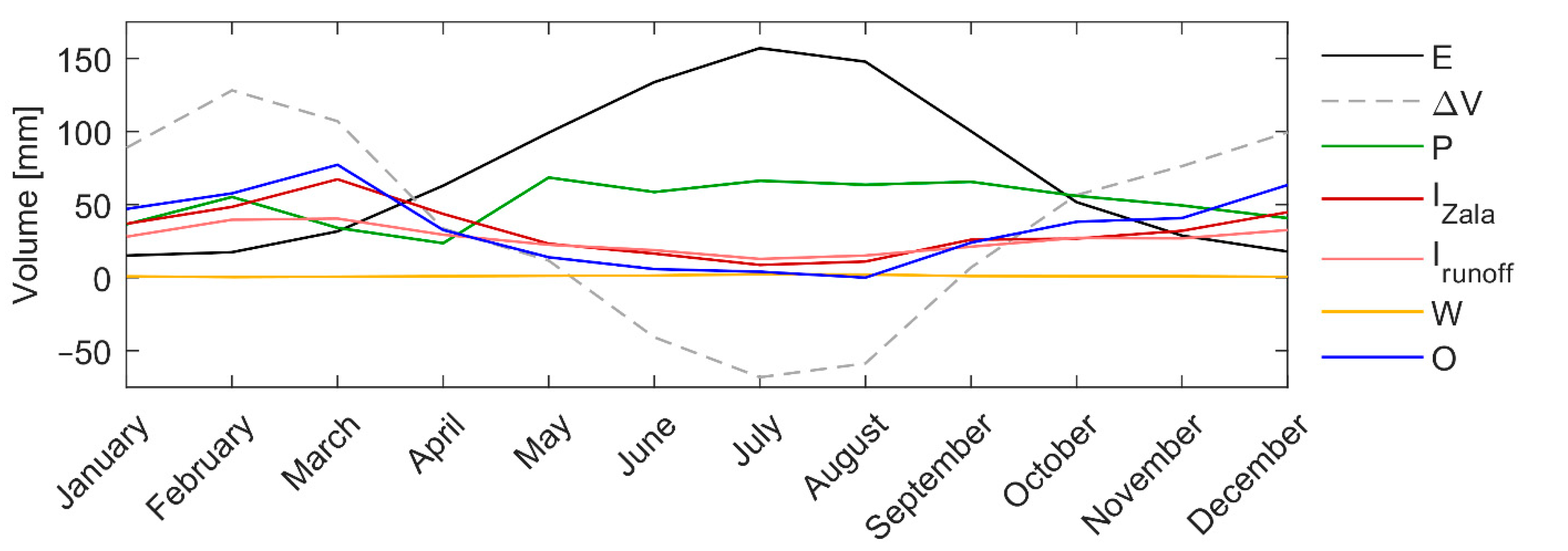
Figure 1. (a) Subcatchments of Lake Balaton with discharge (red dots), precipitation (green triangles) measurement locations, our hydrometeorological measurement station (yellow star) and the HMS (Hungarian Meteorological Service) synoptic meteorological station (white square) and (b) the schematic drawing of our station’s instrumentation.
Atmosphere 13 00352 g001
Figure 2. Water balance components of Lake Balaton. Monthly values represent 11-year means between 2010 and 2020. Water volumes are represented in lake mm (volume divided by the surface area). The components are: E–evaporation, ΔV–water resource change, P–precipitation over the lake, IZala–inflow from Zala River, Istreams–inflow from further streams and sub-catchments, W–water usage, O–outflow through the sluice gate in Siófok.
Atmosphere 13 00352 g002
Figure 3. Time series of 2-h averages of (a) latent (left axis), sensible and sediment heat flux (right axis), (b) net radiative flux, heat storage change and residual of the energy budget, (c) water temperatures, and (d) energy budget closure ratio between 1 August and 15 August in 2019.
Atmosphere 13 00352 g003
Figure 4. The seasonal variation of energy budget components in 2019.
Atmosphere 13 00352 g004
Figure 5. The seasonal variation of energy budget closure (left axis with blue) and Bowen ratio (right axis with red) in 2019.
Atmosphere 13 00352 g005
Figure 6. The monthly (a) mean latent heat fluxes between May and September 2019 provided by the eddy-covariance (EC) observation and the different estimation methods and (b) the relative difference of latent heat fluxes determined by the different methods compared to the EC data.
Atmosphere 13 00352 g006
Figure 7. The latent heat transfer coefficient as a function of wind speed multiplied with the vertical-specific humidity difference.
Atmosphere 13 00352 g007
Figure 8. The seasonal variation of the vapor transfer coefficient (median values) in 2019 with different methods: EC–eddy covariance-based measurements; EB–after closing the energy balance; WB–water balance-based estimations; PM–Penman-Monteith-based estimations; PT–Priestley-Taylor-based estimations.
Atmosphere 13 00352 g008
Figure 9. Monthly probability density functions of roughness lengths for: (a) water vapor (z0q) and (b) sensible heat (z0H) flux based on EC measurements.
Atmosphere 13 00352 g009
Figure 10. Determination coefficients (R2) between different meteorological drivers or energy balance components and (a) the latent heat flux and (b) the vapor transfer coefficient on different time scales.
Atmosphere 13 00352 g010
Figure 11. Intra-annual variation of (a) latent heat flux and (b) water vapor transfer coefficient based on the long-term water balance analysis. Variability of a given month is shown by shading: 10th and 90th percentiles (light grey), 25th and 75th percentiles (dark grey), median values (black lines).
Atmosphere 13 00352 g011
Figure 12. Daily EC measured latent heat fluxes as a function of estimated values using constant (red) and weekly varying (blue) water vapor transfer coefficients for the 2019 measurement period.
Atmosphere 13 00352 g012
Figure 13. Monthly courses between incoming shortwave radiation and (a) latent heat flux and (b) water vapor transfer coefficient based on 11-year water balance data. Whiskers show the 25th and 75th percentiles, while filled circles represent medians.
Atmosphere 13 00352 g013
Figure 14. Determination coefficients (R2) between different meteorological drivers or energy balance components and (a) the sensible heat flux and (b) the heat transfer coefficient on different time scales.
Atmosphere 13 00352 g014
Table 1. Lake Balaton water balance components (means and standard deviations) for the period of detailed hydrometeorological measurements in 2019. Data taken from [37].
[mm]MayJuneJulyAugustSeptember
P123 ± 3065 ± 1667 ± 1756 ± 1428 ± 7
I56 ± 1345 ± 1327 ± 723 ± 615 ± 2
E63 ± 16100 ± 34169 ± 43136 ± 34133 ± 31
O7 ± 223 ± 60 ± 00 ± 00 ± 0
W2 ± 02 ± 02 ± 02 ± 01 ± 0
ΔV108 ± 27−15 ± 4−78 ± 19−59 ± 14−91 ± 22
Publisher’s Note: MDPI stays neutral with regard to jurisdictional claims in published maps and institutional affiliations.

