Abstract
Based on a regional ice-ocean model, we simulated the state of the water masses of the Arctic Ocean to analyze the transport of dissolved methane on the Arctic shelves. From 1970 to 2019, we obtained estimates of methane emissions at the Arctic seas due to the degradation of submarine permafrost and gas release at the ocean–bottom interface. The calculated annual methane flux from the Arctic shelf seas into the atmosphere did not exceed 2 Tg CH4 year−1. We have shown that the East Siberian shelf seas make the main contribution to the total methane emissions of the region. The spatial variability of the methane fluxes into the atmosphere is primarily due to the peculiarities of the water circulation and ice conditions. Only 7% of the dissolved methane originating from sediment enters the atmosphere within the study area. Most of it appears to be transported below the surface and oxidized by microbial activity. We found that increasing periods and areas of ice-free water and decreasing ice concentration have contributed to a steady increase in methane emissions since the middle of the first decade of the current century.
1. Introduction
The dramatic loss of the Arctic Sea ice observed during recent decades is the most apparent manifestation of climate change [1,2,3,4]. As assessed from satellite data in [4], the declining linear trend of the Arctic ice extent for the total 42-year record since 1978 is rated at 40,000 km2 per year. By analyzing linear trends separately for decades, the authors have shown an accelerated decrease in sea ice extent in 2009−2018. According to their findings, the Arctic Sea ice decrease is by 5% in autumn–winter and 35% in spring–summer seasons.
During the last two decades, the most visible changes have occurred in the Arctic Shelves [5]. The Arctic Shelf seas lose sea ice entirely in summer compared to the previous period when they were ice-covered almost all year round. Earlier melting of sea ice and a longer duration of the ice-free period significantly impacts the mass, momentum, and energy exchanges between the atmosphere and the sea surface [3,6]. Additional absorption of heat by the sea surface is followed by the warming of Arctic seawater [7,8,9]. An assessment based on a satellite-derived global daily sea surface temperature data set [10] has shown that the second decade of the 21st century for the Siberian Arctic seas was significantly warmer than the first decade [11]. The authors demonstrated that at the end of the second decade, the Siberian Arctic seas experienced anomalous warming. The surface temperature of these seas reached maximum values exceeding the climatic monthly average and threshold values calculated on the 90th percentile value of daily temperature for the climate period from 1981 to 2010.
Vast reserves of methane associated with the submarine permafrost and methane hydrate deposits [12,13,14] are hidden in the bottom sediments of the Arctic Ocean shelf. They are at risk of decomposition due to rising seabed temperatures, leading to higher methane (CH4) budget in the atmosphere. Estimates of the contribution of oceanic sources of methane (2–40 Teragram per year (Tg/year)) are small compared to land-based sources such as wetlands (153–227 Tg/year), amounting to 80% [15]. However, oceanic sources of CH4 in the Arctic can play a significant role due to the large volumes of methane under the seabed in the permafrost layer and the zone of stability of gas hydrates [16]. Quantifying the release of methane from the seabed and its further emissions into the atmosphere are the main unresolved issues regarding the marine methane cycle.
Glacial cycles led to periods of transgressions and regressions of the seas of the Arctic Ocean during the Pleistocene. Continental permafrost was formed on the Arctic shelf during periods of sea regression when the shelf became dry land [12,17,18]. During the subsequent rise in sea level, such permafrost found itself underwater. The submarine permafrost formed during the Pleistocene glaciation periods can be distributed over a significant part of the Arctic shelf with water depths of up to 120–150 m (depending on the paleogeographic reconstructions), submerged due to the last postglacial transgression [18,19,20]. The formation of a sufficiently thick layer of seawater over permafrost leads to an increase in temperature at their upper boundary, contributing to the degradation of permafrost since its inundation [12,21,22,23]. The submarine permafrost layer acts as a barrier to the underlying methane, which can be in the gaseous state or the form of hydrates. Therefore, the permafrost degradation leads to the methane obtained from the permafrost release and opens up pathways for gas migration from the underlying layers [24]. Methane hydrates are a combination of methane and water, which are stable at high pressures and low temperatures [25,26]. Relict hydrates associated with submarine permafrost are more sensitive to changes than hydrates on land or in the deep ocean. The submarine permafrost layer degrades after flooding, and the conditions for hydrate stability are violated [14,27,28].
In recent years, the East Siberian Arctic Shelf (ESAS) has attracted attention as a significant source of methane to the atmosphere [29,30]. Areas of intensive methane discharge identified on the shelf of the Laptev Sea are one of the main signs of the presence of methane seeps. Measurement data show an increase in methane emissions into the atmosphere of the Arctic region [29,30,31]. This process can be a sequel to an increase in the permeability of the permafrost layer of bottom sediments and gas release from the underlying layers [24,32,33]. Methane hydrate deposits degradation is also called a possible cause [29]. The region’s inaccessibility limits the analysis of methane emissions from the Arctic Ocean seas shelf, especially in the winter. Methane emissions estimates are characterized by high uncertainty [30,34,35,36,37,38,39].
The limited data coverage leads to significant uncertainty in assessing the contribution of the Arctic seas to annual methane emissions. When determining the budget of CH4 entering the atmosphere from the Arctic seas, the estimates of different authors differ markedly. According to [29,30], the rate of methane release from the seas of the East Siberian Arctic Shelf (ESAS) into the atmosphere, estimated based on measurements of the concentration of dissolved CH4 in surface waters, was 8–17 Tg/year. Meanwhile, simultaneous measurements of methane in the atmosphere above the surface and the surface waters of the Laptev and East Siberian Seas in the summer of 2014 gave the maximum estimate of 2.9 Tg/year [34]. In [38], the authors limited the rate of methane emission from the ESAS using data on its atmosphere concentration and an atmospheric transport model. The proposed range for the annual methane flux was 0–4.5 Tg/year. The Intergovernmental Panel on Climate Change (IPCC50 WG1 AR6) concluded that the total methane flux from the surface of all (including both the Arctic Ocean and other oceans) shelf areas to the atmosphere is less than 10 Tg/year [40].
Estimates of annual and winter methane emissions can be obtained using numerical ocean models [41,42]. The use of three-dimensional numerical ocean models makes it possible to estimate and describe the variability of methane fluxes into the atmosphere. This approach makes it possible to assess the impact of various processes in the ocean and sea ice on the transfer of methane from bottom sediments to the atmosphere. It also makes it possible to evaluate the variability of these processes over time.
The purpose of our study is to obtain a model estimate of methane emissions from the Arctic shelf seas into the atmosphere as a result of an increase in the permafrost permeability. This goal includes quantifying spatio-temporal methane emissions and understanding their relationship to the current ocean and ice changes. Our paper is organized as follows: Section 2 describes numerical models and methods used to simulate the Arctic Seas water and ice variability and estimate CH4 emissions. We show the results of the modeling study in Section 3. We discuss the comparison of our results with other work and this study’s main limitations in Section 4. We summarize key research findings in Section 5.
2. Materials and Methods
2.1. Coupled Ice–Ocean Model
The three-dimensional coupled numerical model of the ocean and sea ice SibCIOM (Siberian coupled ice–ocean model) [43,44,45] is used to study the variability of the state of the waters and sea ice of the Arctic Ocean and its shelf seas. The numerical ocean model is based on nonlinear equations of ocean hydrodynamics, taking into account the traditional hydrostatic and Boussinesque approximations.
For some physical processes that we parametrized, the numerical model cannot be adequately resolved; for example, we used parameterization of vertical convective and turbulent mixing [46,47], isopycnal diffusion [48], formation of slope flows, or cascading [49]. This study used the basic parameterization of vertical mixing [46], which eliminates seawater layers’ instability caused by autumn–winter cooling and wind forcing. The vertical adjustment based on the analysis of the Richardson number establishes the uniform distribution of temperature, salinity, velocity profiles, and other tracers included in the model (dissolved methane in this study), taking into account the mass and momentum conservation laws. It is allowed to consider other parameterizations, using modules from the GOTM (General Ocean Turbulence Model, GOTM, [50]) coupled to SibCIOM. However, a comparison of the numerical experiments carried out using the GOTM package models [47] did not reveal the highest priority parameterization of vertical mixing for the Arctic Ocean model.
The ocean model is coupled to adapted the Los Alamos Ice Model CICE [51] included the rheology and multi-category sea-ice thermodynamics modeling [52] and sea-ice advection based on a semi-lagrangian scheme [53].
A feature of the ice regime of the Siberian Arctic seas is the existence of fast ice [54], which is motionless ice on a shelf about eight months a year. In the model, to parameterize the fast ice, we analyze the ice thickness during the time step, and when it achieves 10% of the sea depth, we set the ice drift velocity to be zero at this point of the grid. The simulated fast ice in the summer becomes free moving when the melting rate at the ice bottom is more than 0.1 cm/day.
The modeling area includes the Atlantic Ocean above 20 S latitude and the Arctic Ocean, bounded at the latitude of the Bering Strait. These boundaries and river mouths are considered “liquid” where information about climatic values of temperature, salinity, and transport rate was used. The values recommended in [55] were used to set the transport rate, temperature, and salinity of the waters entering the Bering Strait. On the southern border of the region, free flow is assumed, and the use of climatic values of temperature and salinity in the case of the formation of currents, directed to the inside of the region. Using a three-polar numerical grid, the spatial resolution of the model is 50 km outside the polar zone, 25 km in the deep-water part of the Arctic Ocean, and 15 km in the shelf area. The design of the numerical experiment involves the study of the ocean and sea-ice response to the atmosphere state variability. For the study, a numerical simulation was carried out from January 1948 to December 2019 using the NCEP/NCAR atmospheric reanalysis data provided by the National Oceanic and Atmospheric Administration (NOAA) [56]. Climate data [57] on temperature and salinity distribution for the winter period were used as initial fields.
2.2. Tracer Model
Methane is considered a passive tracer entering the water from the sea bottom. Sea currents transport dissolved methane in the same way as for temperature and salinity. The distribution of dissolved methane (C, in nmol/L, subsequently nM) in seawater is considered as a solution to the advective-diffusion equation for an admixture:
where t is time; U is the water velocity; Diff describes the process of horizontal and vertical diffusion based on second-order operators; Cox is the methane sink term due to its oxidation.
Methane, which dissolves in water, can be oxidized by bacteria to CO2. Thus, the methane oxidation in the water column is the prime sink for methane before it escapes into the atmosphere. Methane oxidation rates were calculated assuming first-order kinetics [42,58]: Cox = Kox·C. The available data show a large scatter of aerobic methane oxidation rates over several orders of magnitude [59]. By analogy with [42], we used a constant rate of methane oxidation, which corresponds to the measured data in the Beaufort Sea, Alaska: Kox = 0.01 day−1. It corresponds to a methane lifetime in seawater of about 100 days. Measured averaged rate constants (Kox) were also on the order of 0.01 day−1 at 40 m water depth in the central North Sea [58].
The horizontal diffusion coefficient can range from 0.1 to 1000 m2/s depending on the proximity to the coast and exponentially increases with distance from the land [58]. Since we set the methane fluxes from the bottom for the shelf with a water depth of less than 120 m (see Section 2.3), the horizontal diffusion coefficient was taken equal to 1 m2/s. The based coefficient of vertical turbulent diffusion can vary from 10−3 to 10−6 m2/s, depending on the stratification [59], and we have taken 10−5 m2/s. Unstable water stratification, simulated during autumn–winter cooling, and wind forcing promote additional mixing in ocean model and the formation of a homogeneously mixed layer for all hydrological characteristics, including the distribution of methane.
An assessment of the methane flux at the sea–air interface is carried out according to the method [60,61], based on the experimentally established parameterizations for the World Ocean. The methane flux into the atmosphere is a function of the difference between the calculated concentration of dissolved methane in the surface water layer CW (in nM) and the equilibrium dissolved methane concentration at the surface CA (in nM), the gas exchange coefficient at the sea–air interface k, and ice concentration KICE in the oceanic cell:
F = k∙(CW − CA)(1 − KICE).
According to the method [62], we calculate the equilibrium methane concentration in seawater (CA) at a given temperature, salinity, and atmospheric pressure. The equilibrium methane concentration calculated by this method was from 3 to 4.5 nM for the Arctic Ocean. The oversaturation of the surface layer of seawater with dissolved methane leads to the release of methane into the atmosphere. Atmospheric methane concentrations are needed to calculate the diffusion flux of methane. Atmospheric methane concentrations range from 1.896 to 1.911 ppm [39], according to the Tiksi weather station database. Similar values were obtained in summer 2014 for the Laptev Sea (1.879 ppm) [34]. In our study, we used atmospheric methane concentration 1.9 ppm.
Gas transfer rate between ocean and atmosphere:
where V is the wind velocity at 10 m (m/s), Sc is the Schmidt number, the non-dimensional ratio of gas diffusivity, and water kinematic viscosity. The coefficient 677 is the Schmidt number for CH4 at 20 °C and salinity 35‰ [60]. When calculating Sc, we use parameterization [61]:
where Tw is the sea surface temperature in °C. Accordingly, in addition to the methane concentration in the surface water, ice concentration, wind velocity, and water temperature are the main factors that determine the methane flux between the ocean and the atmosphere.
k = 0.31 V2∙(Sc/677)−0.5,
Sc = 2101.2 − (131.54(Tw − 273.15)) + (4.4931(Tw − 273.15))2 − (0.08676(Tw − 273.15))3 + (0.00070663 × (Tw − 273.15))4,
2.3. Spatial Distributions of Submarine Permafrost and Model Sources of Methane
Beneath the surface sediment layer, the carbon-rich submarine permafrost formed in the Pleistocene may serve as the base source of methane in the region’s atmosphere. Frozen sediments are a substrate for biogenic CH4. Methane can also migrate upward from dissociating hydrates or free gas deposits due to increased permafrost permeability. The modeling results show that current permafrost is degrading due to flooding during the Holocene transgression by warm ocean waters [21,24,32].
Figure 1 shows the distribution of submarine permafrost in the Arctic previously modeled for the shelf area with a water depth of less than 120 m [14,19]. The distribution of submarine permafrost in the sediments of the shelf covers a total area of 2.5 × 10⁶ km2. We note that the distribution of submarine permafrost (Figure 1) is generally consistent with alternative simulation [18].
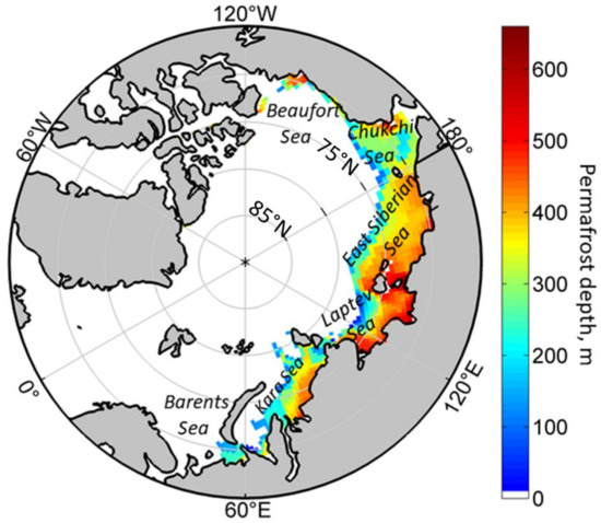
Figure 1.
The distribution and the depth of the modeled submarine permafrost beneath the Arctic Ocean Shelf seas (modified after [14,19]). The diffusion methane flux from the bottom to water is 30 mg/m2 per day in colored ocean region.
In the model calculation at the lower boundary of the ocean in the presence of a permafrost layer in the bottom sediments of the shelf (Figure 1) we set the diffusion flux of methane, 30 mg/m2 per day. This flux corresponds to the maximum values obtained based on measurement data [63] and is associated with permafrost degradation. Average rates of methane release (3–30 mg (CH4)/(m2 day)) are determined by methanogenesis in combination with partial release of preformed gas from relict hydrates preserved in permafrost [63]. For the rest of the ocean, the methane flux at the lower boundary of the ocean is set to 0 mg/m2 per day. The methane sources are set on the bottom of the Arctic shelves, namely: on the part of the Barents and Kara Sea (West Siberian Shelf), the Laptev Sea, the East Siberian Sea, and the Russian part of the Chukchi Sea (East Siberian Shelf), part of the Chukchi Sea and the Canadian shelf (North American Shelf) (Figure 1).
In this study, we assume that such methane emission is associated with the degradation of submarine permafrost flooded during the Holocene and is typical for this area. We are not trying to link this flux with the rate of permafrost degradation or changes in the bottom water temperature. Furthermore, we do not consider the influence of climate on the sources of methane from bottom sediments. Here, we want to find the relationship of CH4 emissions to the atmosphere with the ocean climate changes.
3. Results
3.1. Sea Ice State from Model Simulations
The numerical model SibCIOM was used previously in numerous studies of interannual and seasonal variability of the water and sea ice of the Arctic Ocean and the Arctic Shelves [11,43,44,45,64]. The simulation results show the main processes related to climatic changes known from the analysis of observations. The most pronounced among them is the significant reduction in the Arctic Sea ice cover in summer. Figure 2a shows the simulated distribution of ice concentration in summer 2019 and the ice edge averaged over the first decade. The vast area of the Arctic shelf seas and the adjacent water area, previously occupied by ice, is ice-free in the recent years of the second decade of the 2000s. The model reproduces this process with a certain degree of error compared to the observations (Figure 2b); however, the modeling results clearly show the primary trend of significant degradation of the ice cover started in the first decade of 2000, which continues to the present day.
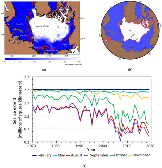
Figure 2.
(a) Sea ice concentration simulated for September 2019. Redline shows minimum ice extent (15%) averaged for 2000–2010. (b) Ice edge position in September 2019. The sea ice extent was obtained using polygon shapefiles derived from publicly available satellite data collected for the period 1981–2020 (National Snow and Ice Data Center; NSIDC Adapted from [65]). (c) Time series of month sea ice extent simulated for February (dark blue), May (blue), August (red), September (violet), October (green), and November (yellow).
Figure 2c shows the time series of the total sea ice area in the ocean shelf, where the methane fluxes from bottom sediments were specified. The total ice area was calculated, taking into account the compactness of the ice. The presented graphs show that since 2004, there has been a reduction in the minimum ice cover area, which is reached in September. In addition, this process continues in October and November. The intense reduction in the ice area in October reflects an increase in the duration of the open water period on the shelf of the Arctic seas [5]. It in turn, leads to an increase in the period of intense heat exchange between the atmosphere and the sea and an increase in wind impact on the water circulation, intensifying surface currents.
The persistent offshore winds, blowing over the Siberian coast in winter and spring, create vast open water area north on the edge of fast ice which is known as the Great Siberian Polynya [54]. In winter, the intensive exchange between the atmosphere and open water leads to surface water cooling and new ice freezing. The numerical model simulates the formation of polynya basically from April to June. In Figure 3, polynya is defined as an area of reduced ice concentration. Its position coincides with the boundary of the shelf zone. Analysis of the temperature and salinity fields carried out based on the monthly average calculated fields shows that in April, the formation of areas of thin ice promotes surface cooling and intense mixing. In June, the numerical model shows the increase in the surface layer temperature in this strip in connection with establishing of positive temperature of the atmosphere and the warming up of the open water area.
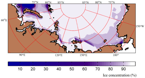
Figure 3.
Simulated sea ice concentration in May 2014. Area of reduced ice concentration in the Laptev and East-Siberian seas shows fast ice polynya.
3.2. Sea Surface Warming in the Arctic Shelf Seas
The model simulates an increase in the temperature of the surface waters of the Arctic shelf seas associated with an intensive reduction in ice cover in the area. An analysis of mean monthly temperature, obtained from numerical experiment, showed that the second decade of this century was warmer for the Siberian Arctic seas than the first decade. Recent years have been extreme in terms of the state of the ice cover and the assessment of the sea surface temperature. Sea surface warming was especially noticeable in the water area of the Kara Sea and the Laptev Sea.
Figure 4a represents the change in the mean monthly surface temperature of the shallow-water part of the Siberian Arctic seas obtained in the numerical experiment. Since 2005, the numerical model simulated summer warming in the surface layer of the shelf seas. In addition, the model shows an increase in the period of maintaining a positive surface temperature, which means an increase in the ice-free period. In the temperature distribution for the East Siberian Sea, an increase in the surface temperature field is also present, but it is less pronounced. Against the general background, only 2007 stands out the most with an abnormally high temperature of surface waters.
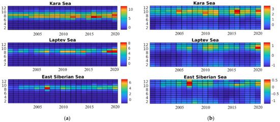
Figure 4.
Monthly temperature change (in °C) in the surface (a) and bottom layer (b) of the Arctic seas. Numerical simulation result.
In Figure 4b, we show the change in the mean monthly temperature of the bottom layer averaged over the shallow-water shelf. In contrast to the surface layer, where the maximum surface temperature values are reached in August, there is no significant warming in the bottom layer this month. In the Laptev and East Siberian Seas, the values of the region-averaged temperature in August do not reach positive values. Analysis of the atmospheric data used as the model forcing and the obtained fields of temperature, salinity, and water circulation shows that anomalously high values of surface temperature in summer over the Arctic seas correspond to the dynamic state of the atmosphere, which contributes to the northward transport of surface warm coastal waters. Figure 5 shows simulated circulation of the surface layer in summer 2019. This off-shore circulation pattern was most often formed in the Kara and Laptev seas in the second decade. In the bottom layer of the sea, the model simulated flow directed from the adjacent regions, particularly from the northern areas to the shelf zone. The presence of fresh river water prevents intensive mixing; as a result, the temperature remains low in the near-bottom layer. In contrast to these seas, in the Kara Sea, the average temperature on the shallow shelf can reach 2 °C in August due to intensive mixing and contact with Atlantic waters.
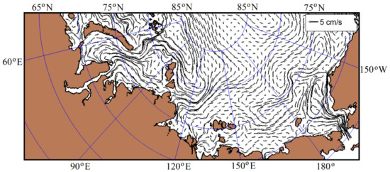
Figure 5.
Circulation of the surface layer in summer 2019. Numerical simulation result.
An increase in the temperature of the bottom layer begins in September, and the maximum temperature is seen, as a rule, in October (Figure 4b). This time shift is explained by the autumn cooling of surface waters and intense mixing, which contributes to heat flow into the deep layers. The numerical model shows that the positive temperature values that have arisen in the bottom layer of the sea due to the previous anomalously warm summer can persist there for several months.
3.3. Dissolved Methane Concentration in Water
We carried out a model analysis of methane emissions into the atmosphere due to gas release at the ocean–bottom interface. The calculated dissolved methane concentrations are maximum (up to 9000 nM) in the bottom water, where CH4 sources are specified. The transfer to the surface depends on the circulation of water masses in a particular period. This transfer is main determined by the seasonal trend and followed a clear time pattern. The highest methane concentrations in the surface layer were obtained in winter and autumn. The lowest CH4 concentrations in the upper water layer were obtained in summer.
The calculated concentrations of dissolved methane in the surface water layer, using the example of 2014, are shown in Figure 6. Despite uniformly specified methane fluxes from the bottom throughout the entire shallow-water shelf, gas rises to the surface only in areas where circulation promoted diffusion and convective transport of methane throughout the water column is formed.
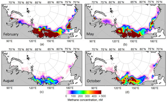
Figure 6.
The maps of dissolved methane concentration at sea surface (in nM) calculated for (a) February, (b) May, (c) August and (d) October 2014.
The maximum methane concentrations in the surface water are typical for the winter months (Figure 6a). The process of concentrations growth occurs together with an increase in the depth of seawater column mixing and begins in the autumn. Due to the water mixing, starting from November, sharp differences in the concentration of dissolved methane in the water column are smoothed out or disappear.
The presence of ice cover prevents the release of gas into the atmosphere during this period. The concentration of CH4 under the ice in the seas of the East Siberian shelf can reach 500–5000 nM (Figure 6a). Dissolved methane is also advected with ocean currents. It is especially noticeable on the outer Arctic shelf (Figure 6a). This process limits the accumulation of CH4 under sea ice and spreads CH4 to other parts of the Arctic Ocean [66]. In winter, the gas accumulated under the ice is oxidized and partially escapes through the ice into the atmosphere.
Ice concentration decrease, the formation of cracks and polynyas leads to the gas release into the atmosphere, and a loss in the concentration of CH4 under the ice in spring (Figure 6b). The rapid ice melt in summer leads to large-scale methane emissions into the atmosphere and a decrease in the CH4 concentration in the surface layer of water to 100–200 nM (Figure 6c). The stable stratification of the Arctic Seas in July–August prevents the rapid influx of CH4 from the bottom water. In this case, the methane concentration in the bottom water can reach more than 9000 nM. The CH4 fraction that reaches the atmosphere without stirring the water column is small. An increase in the methane concentration in the surface layer begins in October simultaneously with an increase in convective processes (Figure 6d).
3.4. Methane Emissions Rates
Methane released from the seabed into the water does not always reach the surface layer and the atmosphere. Part of the methane accumulates in the lower water layer due to the stable stratification and undergoes an oxidation process. Sea ice cover plays a significant role in the methane cycle. In winter, ice cover limits the gas emission into the atmosphere, trapping methane under ice and extending the time of its oxidation in seawater. However, open water is present in sea ice throughout the winter through cracks and polynyas, whose gas can escape into the atmosphere. According to the numerical modeling results, the methane emission in the winter period was 0–2 mg (CH4) m−2 day−1 (Figure 7a–c).
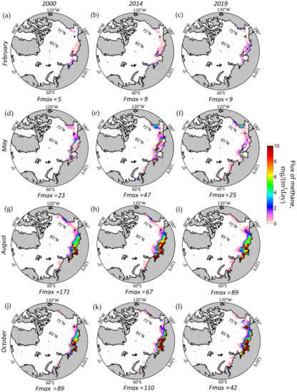
Figure 7.
The maps of methane emissions to the atmosphere (in mg/m2 per day) simulated for the (a–c) February, (d–f) May, (g–i) August and (j–l) October 2000, 2014 and 2019. Fmax is the maximum emission in a given period.
In the spring, the ice is melting, and its concentration decreases, followed by significant emissions of CH4. The model shows the methane flux increase in May at the East Siberian Shelf (Figure 7d–f). The maximum CH4 emission was obtained in the northern part of the Laptev Sea, where polynyas on the edge of fast ice were simulated. It amounted to 23–47 mg (CH4) m−2 day−1, depending on the year. However, the domain of such emissions is insignificant.
The absence of ice cover during the summer months leads to large-scale gas emissions. High fluxes of methane 10–60 mg/(m2 day) are localized in the shallow part of the Laptev Sea shelf (Figure 7g–i). Peak average monthly emissions in August amounted to 171 mg (CH4) m−2 day−1 (western part of the Laptev Sea) in 2000, 67 mg (CH4) m−2 day−1 (southern part of the Laptev Sea, near the Lena Delta) in 2014, and 89 mg (CH4) m−2 day−1 in 2019. In the summer months, methane accumulated under the ice in the winter–spring period is released. In the summer period, the shallow Arctic shelf waters are stratified due to the influx of riverine waters. As a result, a significant part of the dissolved methane can be oxidized in the stratified water column.
An increase in convective mixing, which begins in the autumn months, leads to an increase in the concentration of CH4 in the upper water layer (Figure 6d). Consequently, the area of massive CH4 emission on the shallow shelf has increased, especially in recent years. Therefore, the model CH4 emissions in October 2000, 2014, 2019 are characterized by variability, creating sharp spatial gradients (Figure 7j–l). We obtained high methane fluxes for the southeastern part of the Laptev Sea and the western part of the East Siberian Sea (Figure 7j–l). The later formation of the ice cover contributes to the growth in methane emissions in October 2014 and 2019 compared to the previous periods. First of all, this is due to an increase in the area with increased methane fluxes (Figure 7k,l). In the autumn, the maximum emission rates were obtained in the Laptev Sea near the Lena delta (110 mg (CH4) m−2 day−1). In the East Siberian Sea, the maximum fluxes are in the western part of the sea (80 mg (CH4) m−2 day−1). Methane emissions in other seas are much lower than in the Laptev and East Siberian Seas.
3.5. Estimates of the Annual Methane Emissions
We calculated integral methane fluxes for the entire modeling area on a time scale from one month to a year. The estimate of the total methane flux into the atmosphere as an effect of the degradation of submarine permafrost, obtained in this study, was 0.7–2.0 Tg per year (Figure 8). The estimated methane flux varies more from year to year. Methane emissions have increased significantly over the years. Since 2004, the methane emission into the atmosphere has increased, which, with the assumption of this study constant gas fluxes from bottom sources, may be associated with a decrease in the ice extent in the shelf seas.
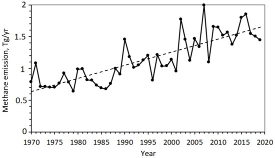
Figure 8.
Annual average net sea–air methane exchange (Teragram per year) obtained in numerical experiment.
In autumn, the methane flux rises due to increased convective mixing and the effect of wind. Nevertheless, when ice covers the water surface in October–November, as it was before 2004, methane emission into the atmosphere in the autumn months remains minimal (Figure 9). Oxidation of methane remaining in the water column in winter significantly reduces CH4 emissions into the atmosphere.
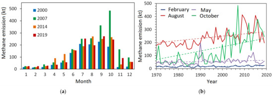
Figure 9.
Methane flux into the atmosphere (kilotons) obtained in a numerical experiment. (a) Flux distribution by months for 2000, 2007, 2014 and 2019. (b) Time series of month methane fluxes for February (dark blue), May (violet), August (red), and October (green). Dotted lines show methane flux trends.
The maximum methane emission into the atmosphere of the Arctic region was obtained for 2007 (Figure 8) which was facilitated by a sharp reduction in the sea ice extent in the autumn period (Figure 2c). If in 2000 the maximum CH4 emission was obtained for the summer months (July–September), then in 2007 it shifts to October (Figure 9a). Since 2004, we have received a trend of increasing methane emissions in October in the Arctic seas (Figure 9b). Continued periods of open water and a decrease in the compactness of the ice cover led to this growth (Figure 2c).
Turbulent diffusion regulates the emission of methane dissolved in water into the atmosphere (1). When calculating the methane flux, turbulence is expressed as a function of wind speed. The Schmidt number for CH4 and gas solubility is a function of the water temperature [61,62]. Thus, besides methane concentration in the surface water, wind speed and water temperature are the key factors determining the methane emission into the atmosphere.
The equilibrium dissolved CH4 concentration (CA) at the surface calculated according to the method described in [62] is shown in Figure 10 for 1996, 2007, and 2019. Its value is approximately 3–4.5 nM for the region under consideration. The rise in temperature in the surface layer of water, obtained in recent years (Figure 4), contributes to a decrease in the solubility of CH4 in water, thereby increasing the amount of gas that can escape into the atmosphere. The increase in the frequency of storms also contributes to increased gas exchange into the atmosphere due to increased wind forces [29].
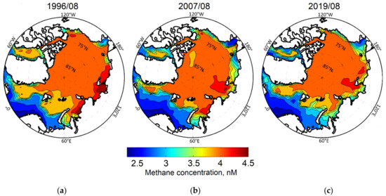
Figure 10.
The equilibrium dissolved CH4 concentration at the sea surface (CA in nM) calculated for simulated temperature and salinity for (a) august 1996, (b) 2007 and (c) 2019.
3.6. Fraction of CH4 That Reaches the Air–Water Interface
The quantitative assessment of methane emissions into the atmosphere is primarily determined by the methane flux from the seabed, which remains uncertain for the entire shelf area. Nevertheless, it is also necessary to understand how much methane will reach the atmosphere. The main barriers to methane release into the atmosphere are CH4 oxidation in seawater, water column stratification, ice conditions, and horizontal transport. The estimate of the CH4 fraction that escapes into the atmosphere is shown in Figure 11. The diffusive methane flux into the atmosphere accounted for 5–10% of the total methane inventory of the study area, depending on the year (Figure 11a). The majority of this fraction (up to 12%) is obtained from the East Siberian Arctic Shelf, with smaller contributions from the West Eurasian (to 2%).
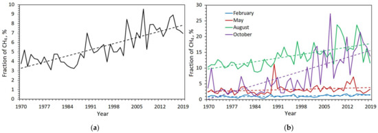
Figure 11.
The fraction of CH4 that reaches the air–water interface and releases into the atmosphere: (a) Time series of average annual methane fraction Arctic Shelf. (b) Time series of the methane fraction for February (blue), May (red), August (green), and October (violet). Dotted lines show trends.
Fraction of CH4, transferred to the atmosphere, was the maximum in summer (up to 24%) and autumn (up to 27%) (Figure 11b). This fraction decreases in winter and spring and is assessed as 1–10% depending on the year (Figure 11b). The loss of the Arctic Sea ice after 2004 leads to an increase in the CH4 fraction that can reach the atmosphere in the autumn months (October, Figure 11b). This process increases the contribution of the autumn–winter CH4 emissions into the total methane flux (Figure 8).
4. Discussion
Based on mathematical modeling, we analyzed the methane emission in the Arctic shelf seas due to gas release at the ocean–bottom interface caused by the degradation of submarine permafrost and an increase in its permeability. In this work, we pursued several goals:
- -
- To assess the fate of methane, which came from bottom sediments into the water column;
- -
- To estimate the amount of CH4 that can reach the atmosphere;
- -
- To see the role of the ocean and sea ice in this process;
- -
- To assess the impact of climatic changes, namely, the reduction in the ice cover, surface water temperature increasing, and wind intensification in recent decades.
To solve these tasks, we used the atmospheric reanalysis data NCEP/NCAR [56] and a three-dimensional numerical model of the ocean and sea ice to simulate inter-annual and seasonal variability of sea ice state, thermohaline, and velocity fields in the Arctic ocean and the Arctic shelf seas. Coupled modeling the state of water masses, ice cover, and transport of dissolved methane allowed us to simulate the spatial and temporal variability of the methane emission from the Arctic shelves.
The numerical coupled ice–ocean model used here is SibCIOM. As a member of the international project FAMOS (Forum for Arctic Modeling & Observational Synthesis, [67]), the model was tested in coordinated modeling studies and compared with observational data [68,69,70]. Recent studies on the SibCIOM simulation [11,45] are closely connected with the present investigation. We have found that sea ice and atmospheric dynamics primarily determine the variability of the Siberian shelf water state. We refer to [11] to show that early ice release and increased air temperature contributed to the formation of an anomalously high surface water temperature for this region, making it possible to consider these events as marine heatwaves [71]. For the present study, the most important is that the model shows the significant reduction in the sea ice cover in summer and sea surface temperature rise at the Siberian shelves during the last years of the second decade of the 2000s.
Especially interesting is the assessment of the impact of the sea ice state using numerical modeling. Indeed, in situ measurements of methane emissions in the Arctic Ocean are carried out onboard ships and in the course of occasional aircraft experiments in July–September. In winter, they are limited by the severe climatic conditions and the region’s inaccessibility.
Numerical simulations have shown that sea ice cover plays an essential role in the Arctic CH4 cycle. On the one hand, ice acts as a barrier between water and the atmosphere, trapping methane in the surface layer, where it can be oxidized or transported by currents (Figure 6a). On the other hand, the formation and melting of sea ice affect the mixing and stratification of the water column and the dynamics of methane transport from the bottom water layer (Figure 6b,d). The intensification of convection in the autumn months leads to a rapid rise of methane from the bottom layer of water to the surface layer. The CH4 concentration under the ice in the seas of the ESAS in our experiments can reach 500–5000 nM (Figure 6a). It is consistent with the work [29], where, according to observational data, high methane concentrations in the surface water layer are recorded in the winter months under the ice in the Laptev Sea. The results of satellite sounding confirm the assumption that the ice cover significantly blocked the flux of methane from the Kara Sea in November–January in the early 2000s, and its decline in subsequent years led to an increase in the methane flux [72].
The interannual variability of simulated methane emissions follows a well-defined scheme, namely, the highest emissions are typical for autumn and summer periods; the lowest emissions are formed in winter; considerable emissions occur during the ice-covered period in the polynyas area. The calculation of the methane flux by the ice concentration allowed us to estimate the methane emission in the winter months. Open water is present in sea ice throughout the winter in the form of cracks and polynyas through which CH4 can be released into the atmosphere during the ice cover period (Figure 7a–f). At the same time, the model average fluxes from the seawater in winter do not exceed 2 mg/m2 per day. The methane emissions increase significantly in April and May when the ice melts and polynyas are formed. In May 2014, the model CH4 fluxes from the polynya were 47 mg/m2 per day (Figure 7e). It is comparable to the methane emission in the summer months during the open-water period (Figure 7h). Measurement data also confirm these results. The Great Siberian Polynya, which remains open at the land–fast-ice interface in the Laptev Sea and the East Siberian Sea, is considered the main pathway for CH4 released into the atmosphere in winter [63]. However, in winter, our estimated CH4 emissions, integrated over the entire shelf area, did not exceed summer flux because the sizes of polynyas are too small compared to the shelf area.
An increase in convective mixing in the autumn leads to growth in CH4 emissions on the shallow-water shelf (Figure 7j–l) especially in recent years due to the later ice cover formation and high wind impact. The obtained results support the assumption of high CH4 emissions from ESAS in autumn due to the intense water column mixing during storms [29].
A comparison of model methane fluxes with observational data [34] confirms the high variability and heterogeneity of methane emissions on the Arctic shelf. The work [34] presents the measurements data of methane fluxes into the atmosphere in the summer period of 2014. The measurements were carried out in the middle and outer shelf with a depth of more than 35 m. The estimates of the average CH4 emission from these data were 4.6, 1.7, and 0.14 mg/(m2 day) in the Laptev, East Siberian, and Chukchi seas, respectively. These average fluxes are in good agreement with the model estimates for a depth of more than 35 m (Figure 7h). Lower values of diffusion fluxes of methane into the atmosphere were obtained from measurements in the areas surrounding the Lena River delta in the Laptev Sea in September 2013 [39]. The calculated CH4 median diffusion fluxes were in the range of 0.06 to 2.6 mg/m2 per day.
The obtained estimate of the methane budget into the atmosphere was 0.7–2.0 Tg per year (Figure 8). The calculated methane flux varies from year to year. Our estimates of the total methane emissions into the atmosphere are consistent with current estimates related to the degradation of the submarine permafrost of the Arctic shelf [34,35,36,38,40].
Many factors affect sea–air gas exchange change due to ongoing climate changes. Reduction in the area of ice cover is one of them (Figure 2). Feedback arises from the decrease in the amount of sea ice. The absence of ice cover increases methane emissions into the atmosphere (Figure 9). We obtained the maximum annual methane emission into the atmosphere in 2007, which was facilitated by a sharp reduction in the area of sea ice in the autumn period (Figure 9b). Extended periods of open water and a decrease in the compactness of the ice cover contribute to a steady increase in CH4 emissions since 2004 (Figure 8, Figure 9 and Figure 11). The results of satellite sounding [72] confirm the results obtained. The authors expressed the opinion that shortly the growth of methane flux from the Arctic Ocean will be largely determined by the process of changing the ice cover of the Arctic [72].
We acknowledge some of the limitations of our research. The quantitative assessment of methane emissions into the atmosphere is first determined by the methane flux from the seabed, which in our case is set uniformly for the entire region. We understand that such an assumption can overestimate sources in some areas and underestimate them in others. Apparently, the CH4 flux can depend on the permafrost degradation rate and on the temperature of bottom seawater, and the geothermal flux, etc. In [29], it was suggested that current climate change is causing an abrupt release of huge amounts of CH4. However, modeling results [24,32,73] show that warming of the Arctic shelf waters has an impact on CH4 emissions due to degradation of permafrost and destabilization of hydrates rather on millennial timescales.
As a source of CH4, we take into account only the diffusion flux of methane from the bottom, which corresponds to the average values obtained based on measurement data [63] and is associated with permafrost degradation. Here, we do not account for the higher methane fluxes associated with fault zones and thermogenic gas outflows. So, surface faults of the outer shelf can create supply channels through which methane migrates to the surface, and its jet is released into the water column [74]. Such a group of faults is observed along the edge of the Laptev Sea shelf [74]. In [63] the authors distinguished between “background” emissions and “hotspots”, presumably associated with large CH4 seeps in talik areas, developing due to geological factors (faults). In such areas, the methane flux into the bottom water is assumed to be from 5 to 24 g/m2 per day, which is several orders of magnitude higher than in our study. On the other hand, in [42] the authors applied a modeling approach that used methane fluxes from ESAS bottom sediments an order of magnitude lower than our estimates, resulting in even lower methane fluxes into the atmosphere.
Thawing submarine permafrost is a source of methane to the subsurface biosphere which can significantly reduce the gas release from the permafrost. Modeled potential anaerobic oxidation consumes 72–100% of submarine permafrost methane and up to 1.2 Tg of carbon per year for the total estimated area [75].
In addition to diffusive air–sea gas transfer, CH4 gas emissions from the seafloor can immediately reach the surface in shallow water shelves during ebullition [30,76]. However, the question of whether this ebullition leads to increased concentrations of methane in the atmosphere remains a matter of controversy. In [35] the authors observed only a few gases boils on the inner shelf. The authors argue that bubbles dominate the CH4 fluxes from the sea to the air only in small limited areas: in an area of ~100 m2 in the East Siberian Sea, the sea–air CH4 fluxes exceed 600 mg/m2 per day; in the Laptev Sea area of a similar size, the peak CH4 fluxes were ~170 mg/m−2 per day. The authors concluded that the CH4 flux into the atmosphere is mainly due to turbulent diffusion. We consider only the diffusion methane flux into the water column; the bubbly emission of CH4 from bottom sediments is not considered. It can lead to underestimating obtained methane emissions from the Arctic shelf rather than its shallowest part (less than 30 m).
Another uncertainty in our study is the constant value for the oxidation rate for CH4 in the water column. The aerobic microbial methane oxidation is essential as it is the only known sink within the oxygenated water column, decreasing the CH4 concentration. Methane oxidation has a significant impact on the net sea–air exchange of CH4 [42]. The methane oxidation rates measured at different locations in the ocean water column broadly differ [59]. Only a few in situ observations are available for the Arctic Ocean [42]. In this study, the oxidation rate constant is consistent with measurements in the Beaufort Sea, Alaska [77], and measured averaged rate constants in the central North Sea [58]. In the future, we will investigate how different measured oxidation rates affect the flux of CH4 to the atmosphere.
A sufficient number of measurements of methane fluxes from the bottom and methane oxidation rates would reduce the uncertainty in estimating methane emissions to the atmosphere.
5. Conclusions
In this work, we pursued two main goals:
- -
- To obtain a model estimate of methane emissions from the seas of the Arctic shelf into the atmosphere due to an increase in the permeability of frozen bottom sediments based on the ice-ocean model.
- -
- To understand the relationship between spatio-temporal methane emissions and ongoing changes in the ocean and ice.
To solve these tasks, we used the method of mathematical modeling. Based on the three-dimensional numerical model of the ocean and sea ice SibCIOM and atmospheric reanalysis data, we simulated changes in hydrography and the ice state of the Arctic ocean and the Arctic shelf seas.
In the numerical experiment, we obtained a significant reduction in the Arctic Sea ice cover in summer and the most intense sea surface warming in the Siberian Arctic seas. According to our estimates, the most intense temperature rise occurred in recent years of the second decade.
Coupled modeling the state of water masses, ice cover, and transport of dissolved methane gave us the opportunity to simulate and analyze the methane emission in the Arctic seas due to gas release at the ocean–bottom interface caused by the degradation of submarine permafrost and an increase in its permeability.
Our estimates of the methane emissions from the seas of the Arctic shelves to the atmosphere are 0.7–2 Tg CH4/year and these estimates are consistent with findings reported in [34,35,36,38,40].
On average, only 7% of the dissolved methane released from the bottom sediments escapes into the atmosphere within the study area. Most of it accumulates in the water layer, is transported by currents, and is oxidized by microbes. It was found that the East Siberian and Laptev seas make the main contribution to the total methane emission in the region.
The obtained methane fluxes spatial variability into the atmosphere is primarily due to the peculiarities of the water circulation and ice conditions. The highest CH4 emissions are in the autumn months. It indicates the role of convective mixing of the water column and a wind speed increase in recent years.
We estimated methane emissions during the ice-covered period. Emissions during this period are associated with areas of open water in the ice cover—cracks and polynyas. The CH4 concentration under the ice in the surface water can reach about 5000 nM. As a result, significant emissions were obtained during the ice-covered period from the areas of polynyas. However, the amount of such emissions is limited by the open water area. More extended open-water periods and reduced ice concentration have contributed to a steady increase in methane emissions since the middle of the first decade of the present century. In the context of the ongoing and projected climate warming, in the coming years, the growth of methane emissions in the Arctic seas will be determined not only by gas fluxes from sediments but also by the process of changing the ice cover of the Arctic.
Author Contributions
Conceptualization, V.M. and E.G.; methodology, V.M. and E.G.; software, E.G. and V.M.; investigation, V.M. and E.G.; writing—review and editing, V.M. and E.G.; visualization, V.M. and E.G.; funding acquisition, V.M. and E.G. All authors have read and agreed to the published version of the manuscript.
Funding
Analysis of climate variability of water and ice state of the Siberian Arctic seas was supported by Russian Science Foundation, grant 20-11-20112. Estimates of the methane emissions from the Arctic seas were funded by Russian Foundation for Basic Research, grant 20-05-00241.
Institutional Review Board Statement
Not applicable.
Informed Consent Statement
Not applicable.
Data Availability Statement
NCEP/NCAR Reanalysis Data are provided by National Centers for Environmental Prediction/National Weather Service—NOAA, U.S. Department of Commerce, NCEP/NCAR Global Reanalysis Products, 1948-continuing, Research Data Archive https://psl.noaa.gov/data/gridded/data.ncep.reanalysis.html (accessed on 1 October 2021). The simulations output used in this paper is available from the first author by request.
Acknowledgments
The authors kindly thank anonymous reviewers for their constructive criticism and suggestions. The Siberian Branch of the Russian Academy of Sciences (SB RAS) Siberian Supercomputer Center is gratefully acknowledged for providing supercomputer facilities.
Conflicts of Interest
The authors declare no conflict of interest. The funders had no role in the design of the study; in the collection, analyses, or interpretation of data; in the writing of the manuscript, or in the decision to publish the results.
References
- Kwok, R.; Cunningham, G.F.; Wensnahan, M.; Rigor, I.; Zwally, H.J.; Yi, D. Thinning and volume loss of the Arctic Ocean sea ice cover: 2003–2008. J. Geophys. Res. 2009, 114, C07005. [Google Scholar] [CrossRef]
- Comiso, J.J. Large decadal decline of the arctic multiyear ice cover. J. Clim. 2012, 25, 1176–1193. [Google Scholar] [CrossRef]
- Collins, M.; Sutherland, M.; Bouwer, L.; Cheong, S.-M.; Frölicher, T.; Jacot Des Combes, H.; Koll Roxy, M.; Losada, I.; McInnes, K.; Ratter, B.; et al. 2019: Extremes, Abrupt Changes and Managing Risk. In IPCC Special Report on the Ocean and Cryosphere in a Changing Climate; Pörtner, H.-O., Roberts, D.C., Masson-Delmotte, V., Zhai, P., Tignor, M., Poloczanska, E., Mintenbeck, K., Alegría, A., Nicolai, M., Okem, A., et al., Eds.; Intergovernmental Panel on Climate Change: Geneva, Switzerland, 2019; Available online: https://www.ipcc.ch/report/srocc/ (accessed on 25 October 2021).
- Yulin, A.V.; Vyazigina, N.A.; Egorova, E.S. Interannual and seasonal variability of Arctic Sea ice extent according to satellite observations. Russ. Arct. 2019, 7, 26–35. (In Russian) [Google Scholar]
- Review of Hydrometeorological Processes in the Arctic Ocean. 2015–2020. (In Russian). Available online: http://www.aari.ru/main.php?lg=0&id=449 (accessed on 25 October 2021).
- Döscher, R.; Vihma, T.; Maksimovich, E. Recent advances in understanding the Arctic climate system state and change from a sea ice perspective: A review. Atmos. Chem. Phys. 2014, 14, 13571–13600. [Google Scholar] [CrossRef]
- Singh, R.K.; Maheshwari, M.; Oza, S.R.; Kumar, R. Long-term variability in Arctic Sea surface temperatures. Polar Sci. 2013, 7, 233–240. [Google Scholar] [CrossRef]
- Timmermans, M.-L.; Labe, Z. Sea Surface Temperature; Arctic Report Card, Update to 2020; National Oceanic and Atmospheric Administration (NOAA): Washington, DC, USA, 2020; pp. 54–58. [CrossRef]
- Hu, S.; Zhang, L.; Qian, S. Marine heatwaves in the Arctic region: Variation in different ice covers. Geophys. Res. Lett. 2020, 47, e2020GL089329. [Google Scholar] [CrossRef]
- Reynolds, R.W.; Smith, T.M.; Liu, C.; Chelton, D.B.; Casey, K.S.; Schlax, M.G. Daily High-Resolution-Blended Analyses for Sea Surface Temperature. J. Clim. 2007, 20, 5473–5496. [Google Scholar] [CrossRef]
- Golubeva, E.; Kraineva, M.; Platov, G.; Iakshina, D.; Tarkhanova, M. Marine Heatwaves in Siberian Arctic Seas and Adjacent Region. Remote Sens. 2021, 13, 4436. [Google Scholar] [CrossRef]
- Romanovskii, N.N.; Hubberten, H.W.; Gavrilov, A.V.; Eliseeva, A.A.; Tipenko, G.S. Offshore permafrost and gas hydrate stability zone on the shelf of East Siberian Seas. Geo-Mar. Lett. 2005, 25, 167–182. [Google Scholar] [CrossRef]
- Ruppel, C. Permafrost-associated gas hydrate: Is it really approximately 1 % of the global system? J. Chem. Eng. Data 2015, 60, 429–436. [Google Scholar] [CrossRef]
- Malakhova, V.V. The response of the Arctic Ocean gas hydrate associated with subsea permafrost to natural and anthropogenic climate changes. IOP Conf. Ser. Earth Environ. Sci. 2020, 606, 012035. [Google Scholar] [CrossRef]
- Kirschke, S.; Bousquet, P.; Ciais, P.; Saunois, M.; Canadell, J.G.; Dlugokencky, E.J.; Bergamaschi, P.; Bergmann, D.; Blake, D.R.; Bruhwiler, L. Three decades of global methane sources and sinks. Nat. Geosci. 2013, 6, 813–823. [Google Scholar] [CrossRef]
- James, R.; Bousquet, P.; Bussmann, I.; Haeckel, M.; Kipfer, R.; Leifer, I.; Niemann, H.; Ostrovsky, I.; Piskozub, J.; Rehder, G.; et al. Effects of climate change on methane emissions from seafloor sediments in the Arctic Ocean: A review. Limnol. Oceanogr. 2016, 61, S283–S299. [Google Scholar] [CrossRef]
- Malakhova, V.; Eliseev, A. Uncertainty in temperature and sea level datasets for the Pleistocene glacial cycles: Implications for thermal state of the subsea sediments. Glob. Planet. Change 2020, 192, 103249. [Google Scholar] [CrossRef]
- Overduin, P.P.; Schneider von Deimling, T.; Miesner, F.; Grigoriev, M.N.; Ruppel, C.D.; Vasiliev, A.; Lantuit, H.; Juhls, B.; Westermann, S. Submarine permafrost map in the Arctic modeled using 1-D transient heat flux (SuPerMAP). J. Geophys. Res. Oceans 2019, 124, 3490–3507. [Google Scholar] [CrossRef]
- Malakhova, V.V. Estimation of the subsea permafrost thickness in the Arctic Shelf. In Proceedings of the 24th International Symposium on Atmospheric and Ocean Optics: Atmospheric Physics, Tomsk, Russia, 2–5 July 2018; SPIE: Bellingham, WA, USA, 2018; Volume 10833. [Google Scholar] [CrossRef]
- Gavrilov, A.; Malakhova, V.; Pizhankova, E.; Popova, A. Permafrost and Gas Hydrate Stability Zone of the Glacial Part of the East-Siberian Shelf. Geosciences 2020, 10, 484. [Google Scholar] [CrossRef]
- Angelopoulos, M.; Overduin, P.; Jenrich, M.; Nitze, I.; Günther, F.; Strauss, J.; Westermann, S.; Schirrmeister, L.; Kholodov, A.; Krautblatter, M.; et al. Onshore thermokarst primes subsea permafrost degradation. Geophys. Res. Lett. 2021, 48, e2021GL093881. [Google Scholar] [CrossRef]
- Schuur, E.; McGuire, A.; Schädel, C.; Grosse, G.; Harden, J.W.; Hayes, D.J.; Hugelius, G.; Koven, C.D.; Kuhry, P.; Lawrence, D.M.; et al. Climate change and the permafrost carbon feedback. Nature 2015, 520, 171–179. [Google Scholar] [CrossRef]
- Sayedi, S.S.; Abbott, B.W.; Thornton, B.F.; Frederick, J.M.; Vonk, J.E.; Overduin, P.; Schädel, C.; Schuur, E.A.G.; Bourbonnais, A.; Demidov, N.; et al. Subsea permafrost carbon stocks and climate change sensitivity estimated by expert assessment. Environ. Res. Lett. 2020, 15, 124075. [Google Scholar] [CrossRef]
- Dmitrenko, I.; Kirillov, S.; Tremblay, L.; Kassens, H.; Anisimov, O.; Lavrov, S.; Razumov, S.; Grigoriev, M. Recent changes in shelf hydrography in the Siberian Arctic: Potential for subsea permafrost instability. J. Geophys. Res. Oceans 2011, 116, C10027. [Google Scholar] [CrossRef]
- Kvenvolden, K.A.; Lilley, M.D.; Lorenson, T.D.; Barnes, P.W.; McLaughlin, E. The Beaufort Sea continental shelf as a seasonal source of atmospheric methane. Geophys. Res. Lett. 1993, 20, 2459–2462. [Google Scholar] [CrossRef]
- Ruppel, C.D.; Kessler, J.D. The interaction of climate change and methane hydrates. Rev. Geophys. 2017, 55, 126–168. [Google Scholar] [CrossRef]
- Mestdagh, T.; Poort, J.; De Batist, M. The sensitivity of gas hydrate reservoirs to climate change: Perspectives from a new combined model for permafrost-related and marine settings. Earth Sci. Rev. 2017, 169, 104–131. [Google Scholar] [CrossRef]
- Majorowicz, J.A.; Safanda, J.; Osadetz, K. Inferred gas hydrate and permafrost stability history models linked to climate change in the Beaufort-Mackenzie Basin, Arctic Canada. Clim. Past 2012, 8, 667–682. [Google Scholar] [CrossRef]
- Shakhova, N.E.; Semiletov, I.P.; Leifer, I.; Sergienko, V.; Salyuk, A.; Kosmach, D.; Chernykh, D.; Stubbs, C.; Nicolsky, D.; Tumskoy, V.; et al. Ebullition and storm-induced methane release from the East Siberian Arctic Shelf. Nat. Geosci. 2014, 7, 64–70. [Google Scholar] [CrossRef]
- Shakhova, N.E.; Semiletov, I.P.; Salyuk, A.; Yusupov, V.; Kosmach, D.; Gustafsson, O. Extensive Methane Venting to the Atmosphere from Sediments of the East Siberian Arctic Shelf. Science 2010, 327, 1246–1250. [Google Scholar] [CrossRef]
- Pankratova, N.; Skorokhod, A.; Belikov, I.; Elansky, N.; Rakitin, V.; Shtabkin, Y.; Berezina, E. Evidence of atmospheric response to methane emissions from the East Siberian Arctic Shelf. Geogr. Environ. Sustain. 2018, 11, 85–92. [Google Scholar] [CrossRef]
- Malakhova, V.; Golubeva, E. Estimation of the permafrost stability on the East Arctic shelf under the extreme climate warming scenario for the XXI century. Ice Snow 2016, 56, 61–72. [Google Scholar] [CrossRef]
- Frederick, J.M.; Buffett, B.A. Taliks in relic submarine permafrost and methane hydrate deposits: Pathways for gas escape under present and future conditions. J. Geophys. Res. Earth 2014, 119, 106–122. [Google Scholar] [CrossRef]
- Thornton, B.F.; Geibel, M.C.; Crill, P.M.; Humborg, C.; Mörth, C.-M. Methane fluxes from the sea to the atmosphere across the Siberian shelf seas. Geophys. Res. Lett. 2016, 43, 5869–5877. [Google Scholar] [CrossRef]
- Thornton, B.F.; Prytherch, J.; Andersson, K.; Brooks, I.M.; Salisbury, D.; Tjernström, M.; Crill, P.M. Shipborne eddy covariance observations of methane fluxes constrain Arctic Sea emissions. Sci. Adv. 2020, 6, eaay7934. [Google Scholar] [CrossRef] [PubMed]
- Tohjima, Y.; Zeng, J.; Shirai, T.; Niwa, Y.; Ishidoya, S.; Taketani, F.; Sasano, D.; Kosugi, N.; Kameyama, S.; Takashima, H.; et al. Estimation of CH4 emissions from the East Siberian Arctic Shelf based on atmospheric observations aboard the R/V Mirai during fall cruises from 2012 to 2017. Polar Sci. 2020, 27, 100571. [Google Scholar] [CrossRef]
- Fenwick, L.; Capelle, D.; Damm, E.; Zimmermann, S.; Williams, W.J.; Vagle, S.; Tortell, P.D. Methane and nitrous oxide distributions across the North American Arctic Ocean during summer, 2015. J. Geophys. Res. Oceans 2017, 122, 390–412. [Google Scholar] [CrossRef]
- Berchet, A.; Bousquet, P.; Pison, I.; Locatelli, R.; Chevallier, F.; Paris, J.-D.; Dlugokencky, E.J.; Laurila, T.; Hatakka, J.; Viisanen, Y.; et al. Atmospheric constraints on the methane emissions from the East Siberian shelf. Atmos. Chem. Phys. 2016, 16, 4147–4157. [Google Scholar] [CrossRef]
- Bussmann, I.; Hackbusch, S.; Schaal, P.; Wichels, A. Methane distribution and oxidation around the Lena Delta in summer 2013. Biogeosciences 2017, 14, 4985–5002. [Google Scholar] [CrossRef]
- Canadell, J.; Monteiro, P.; Costa, M.; Cotrim da Cunha, L.; Cox, P.; Eliseev, A.; Henson, S.; Ishii, M.; Jaccard, S.; Koven, C.; et al. Global carbon and other biogeochemical cycles and 400 feedbacks. In Climate Change 2021: The Physical Science Basis. Contribution of Working Group I to the Sixth Assessment Report of the Intergovernmental Panel on Climate Change; Masson-Delmotte, V., Zhai, P., Pirani, A., Connors, S., Péan, C., Berger, S., Caud, N., Chen, Y., Goldfarb, L., Gomis, M., et al., Eds.; Cambridge University Press: Cambridge, UK; New York, NY, USA, 2021. [Google Scholar]
- Malakhova, V.V.; Golubeva, E.N. On possible methane emissions from the East Arctic Sea. Atmos Ocean. Opt. 2013, 26, 452–458. (In Russian) [Google Scholar]
- Wåhlström, I.; Meier, H.E.M. A model sensitivity study for the sea-air exchange of methane in the Laptev Sea, Arctic Ocean. Tellus Ser. B Chem. Phys. Meteorol. 2014, 66, 24174. [Google Scholar] [CrossRef]
- Golubeva, E.N.; Platov, G.A. Numerical modeling of the Arctic Ocean Ice System Response to Variations in the Atmospheric Circulation from 1948 to 2007. Izv. Atmos. Ocean. Phys. 2009, 45, 137–151. [Google Scholar] [CrossRef]
- Platov, G.A.; Golubeva, E.N.; Kraineva, M.V.; Malakhova, V.V. Modeling of climate tendencies in Arctic seas based on atmospheric forcing EOF decomposition. Ocean. Dyn. 2019, 69, 747–767. [Google Scholar] [CrossRef]
- Golubeva, E.; Platov, G.; Malakhova, V.; Kraineva, M.; Iakshina, D. Modelling the Long-Term and Inter-Annual Variability in the Laptev Sea Hydrography and Subsea Permafrost State. Polarforschung 2017, 87, 195–210. [Google Scholar] [CrossRef]
- Golubeva, E.N.; Ivanov, J.A.; Kuzin, V.I.; Platov, G.A. Numerical modeling of the World Ocean circulation including upper ocean mixed layer. Oceanol. Engl. Transl. 1992, 32, 395–405. [Google Scholar]
- Iakshina, D.F.; Golubeva, E.N. Influence of the vertical mixing parameterization on the modeling results of the Arctic Ocean hydrology. Proc. SPIE 2017, 10466, 1046657. [Google Scholar] [CrossRef]
- Iakshina, D.F.; Golubeva, E.N. Sensitivity study of a warm Atlantic layer to diffusion parametrization in the Arctic modeling. Bull. Nov. Comp. Center 2014, 14, 1–15. [Google Scholar]
- Platov, G.A. Numerical modeling of the Arctic Ocean deepwater formation: Part II. Results of regional and global experiments. Izv. Atmos. Ocean. Phys. 2011, 47, 377–392. [Google Scholar] [CrossRef]
- Burchard, H.; Bolding, K.; Villarreal, M.R. GOTM, a General Ocean Turbulence Model: Theory, Implementation and Test Cases. Tech. Rep. EUR 18745,103, EN; European Commission: Brussels, Belgium, 1999; Available online: https://gotm.net (accessed on 8 December 2021).
- Hunke, E.C.; Dukowicz, J.K. An elastic-viscous-plastic model for ice dynamics. J. Phys. Oceanogr. 1997, 27, 1849–1867. [Google Scholar] [CrossRef]
- Bitz, C.M.; Lipscomb, W.H. An energy-conserving thermodynamic model of sea ice. J. Geophys. Res. 1999, 104, 15669–15677. [Google Scholar] [CrossRef]
- Lipscomb, W.H.; Hunke, E.C. Modeling Sea Ice Transport Using Incremental Remapping. Mon. Weather Rev. 2004, 132, 1341–1354. [Google Scholar] [CrossRef]
- Zakharov, V.F. The role of flaw leads off the edge of fast ice in the hydrological and ice regime of the Laptev Sea. Oceanol. Engl. Transl. 1966, 6, 815–821. [Google Scholar]
- Woodgate, R.A. Increases in the Pacific inflow to the Arctic from 1990 to 2015, and insights into seasonal trends and driving mechanisms from year-round Bering Strait mooring data. Prog. Oceanogr. 2018, 160, 124–154. [Google Scholar] [CrossRef]
- Kalnay, E.; Kanamitsu, M.; Kistler, R.; Collins, W.; Deaven, D.; Gandin, L.; Iredell, M.; Saha, S.; White, G.; Woollen, J.; et al. The NCEP/NCAR 40-Year Reanalysis Project. Bull. Amer. Meteor. Soc. 1996, 77, 437–471. [Google Scholar] [CrossRef]
- Steele, M.; Morley, R.; Ermold, W. PHC: A global hydrography with a high quality Arctic Ocean. J. Clim. 2000, 14, 2079–2087. [Google Scholar] [CrossRef]
- Mau, S.; Gentz, T.; Körber, J.-H.; Torres, M.E.; Römer, M.; Sahling, H.; Wintersteller, P.; Martinez, R.; Schlüter, M.; Helmke, E. Seasonal methane accumulation and release from a gas emission site in the central North Sea. Biogeosciences 2015, 12, 5261–5276. [Google Scholar] [CrossRef]
- Mau, S.; Blees, J.; Helmke, E.; Niemann, H.; Damm, E. Vertical distribution of methane oxidation and methanotrophic response to elevated methane concentrations in stratified waters of the Arctic fjord Storfjorden (Svalbard, Norway). Biogeosciences 2013, 10, 6267–6278. [Google Scholar] [CrossRef]
- Wanninkhof, R.; Asher, W.E.; Ho, D.T.; Sweeney, C.; McGillis, W.R. Advances in quantifying air-sea gas exchange and environmental forcing. Ann. Rev. Mar. Sci. 2009, 1, 213–244. [Google Scholar] [CrossRef]
- Wanninkhof, R. Relationship between wind speed and gas exchange over the ocean revisited. Limnol. Oceanogr. Meth. 2014, 12, 351–362. [Google Scholar] [CrossRef]
- Wiesenburg, D.A.; Guinasso, N.L., Jr. Equilibrium solubilities of methane, carbon monoxide, and hydrogen in water and sea water. J. Chem. Eng. Data 1979, 24, 356–360. [Google Scholar] [CrossRef]
- Shakhova, N.; Semiletov, I.; Sergienko, V.; Lobkovsky, L.; Yusupov, V.; Salyuk, A.; Salomatin, A.; Chernykh, D.; Kosmach, D.; Panteleev, G.; et al. The East Siberian Arctic Shelf: Towards further assessment of permafrost-related methane fluxes and role of sea ice. Philos. Trans. R. Soc. A 2015, 373, 20140451. [Google Scholar] [CrossRef] [PubMed]
- Golubeva, E.; Kraineva, M.; Platov, G. Simulation of near-bottom water warming in the Laptev Sea. IOP Conf. Ser. Earth Environ. Sci. 2020, 611, 012010. [Google Scholar] [CrossRef]
- National Snow and Ice Data Center: Sea Ice Index. Available online: https://nsidc.org/data/seaice_index/archives (accessed on 20 June 2021).
- Damm, E.; Bauch, D.; Krumpen, T.; Rabe, B.; Korhonen, M.; Vinogradova, E.; Uhlig, C. The Transpolar Drift conveys methane from the Siberian Shelf to the central Arctic Ocean. Sci. Rep. 2018, 8, 4515. [Google Scholar] [CrossRef] [PubMed]
- Proshutinsky, A.; Steele, M.; Timmermans, M.-L. Forum for Arctic Modeling and Observational Synthesis (FAMOS): Past, current, and future activities. J. Geophys. Res. Ocean. 2016, 121, 3803–3819. [Google Scholar] [CrossRef]
- Timmermans, M.-L.; Proshutinsky, A.; Golubeva, E.; Jackson, J.M.; Krishfield, R.; McCall, M.; Platov, G.; Toole, J.; Williams, W.; Kikuchi, T.; et al. Mechanisms of Pacific summer water variability in the Arctic’s Central Canada Basin. J. Geophys. Res. Ocean. 2014, 119, 7523–7548. [Google Scholar] [CrossRef]
- Proshutinsky, A.; Krishfield, R.; Toole, J.M.; Timmermans, M.-L.; Williams, W.; Zimmermann, S.; Yamamoto-Kawai, M.; Armitage, T.W.K.; Dukhovskoy, D.; Golubeva, E.; et al. Analysis of the Beaufort Gyre freshwater content in 2003–2018. J. Geophys. Res. Oceans 2019, 124, 9658–9689. [Google Scholar] [CrossRef] [PubMed]
- Aksenov, Y.; Karcher, M.; Proshutinsky, A.; Gerdes, R.; de Cuevas, B.; Golubeva, E.; Kauker, F.; Nguyen, A.T.; Platov, G.A.; Wadley, M.; et al. Arctic pathways of Pacific Water: Arctic Ocean Model Intercomparison experiments. J. Geophys. Res. Oceans 2016, 121, 27–59. [Google Scholar] [CrossRef]
- Hobday, A.J.; Alexander, L.V.; Perkins, S.E.; Smale, D.A.; Straub, S.C.; Oliver, E.C.J.; Benthuysen, J.A.; Burrows, M.T.; Donat, M.G.; Feng, M.; et al. A hierarchical approach to defining marine heatwaves. Prog. Oceanogr. 2016, 141, 227–238. [Google Scholar] [CrossRef]
- Yurganov, L.N. The relationship between methane transport to the atmosphere and the decay of the Kara Sea ice cover: Satellite data for 2003–2019. Ice Snow 2020, 60, 423–430. [Google Scholar] [CrossRef]
- Wilkenskjeld, S.; Miesner, F.; Overduin, P.; Puglini, M.; Brovkin, V. Strong increase of thawing of subsea permafrost in the 22nd century caused by anthropogenic climate change. Cryosphere Discuss. 2021, 2021, 1–18. [Google Scholar] [CrossRef]
- Baranov, B.; Galkin, S.; Vedenin, A.; Vedenin, A.; Dozorova, K.; Gebruk, A.; Flint, M. Methane seeps on the outer shelf of the Laptev Sea: Characteristic features, structural control, and benthic fauna. Geo. Mar. Lett. 2020, 40, 541–557. [Google Scholar] [CrossRef]
- Winkel, M.; Mitzscherling, J.; Overduin, P.P.; Horn, F.; Winterfeld, M.; Rijkers, R.; Grigoriev, M.N.; Knoblauch, C.; Mangelsdorf, K.; Wagner, D.; et al. Anaerobic methanotrophic communities thrive in deep submarine permafrost. Sci. Rep. 2018, 8, 1291. [Google Scholar] [CrossRef] [PubMed]
- Leifer, I.; Luyendyk, B.P.; Boles, J.; Clark, J.F. Natural marine seepage blowout: Contribution to atmospheric methane. Glob. Biogeochem. Cycles 2006, 20, GB3008. [Google Scholar] [CrossRef]
- Lorenson, T.D.; Kvenvolden, K.A. Methane in Coastal Water, Sea Ice, and Bottom Sediments, Beaufort Sea, Alaska; Open-File Report 95–70; U.S. Department of the Interior, U.S. Geological Survey: Menlo Park, CA, USA, 1995.


Publisher’s Note: MDPI stays neutral with regard to jurisdictional claims in published maps and institutional affiliations. |
© 2022 by the authors. Licensee MDPI, Basel, Switzerland. This article is an open access article distributed under the terms and conditions of the Creative Commons Attribution (CC BY) license (https://creativecommons.org/licenses/by/4.0/).